Prediction of Bridge Structural Response Based on Nonstationary Transformer
Abstract
Accurate prediction of bridge structural responses is crucial for infrastructure safety and maintenance. This study introduces the Nonstationary Transformer (NSFormer), a novel model designed to address the challenges posed by nonstationary data in bridge monitoring, characterized by trends, periodicity, and random fluctuations. Unlike traditional models such as LSTM and Transformer, NSFormer leverages a de-stationary attention mechanism that dynamically adapts to changing temporal patterns, enabling robust long-term prediction. Experimental results show that NSFormer consistently outperforms the traditional models across multiple datasets and prediction horizons. Specifically, at a 24-step prediction horizon, NSFormer reduces mean absolute error by at least 22.88% for Deflection dataset and 66.67% for Strain-All dataset. While predictive accuracy decreases with longer horizons, NSFormer maintains superior performance compared to alternatives. Furthermore, prediction accuracy remains stable across varying input horizons, demonstrating the model’s ability to effectively capture temporal dependencies despite data variability. These findings imply that NSFormer can significantly enhance the reliability of structural health monitoring systems by providing more accurate and stable prediction under complex, variable conditions, thereby supporting timely maintenance decisions and improving bridge safety management.
1. Introduction
With the increasing focus on the safety of buildings and structures, structural health monitoring (SHM) technology has become an important research direction in the engineering field and has been widely applied [1–4]. SHM technology involves long-term, real-time, and scientific monitoring of structures during their operational phase, enabling the timely identification of potential safety hazards, thereby ensuring the health and safety of the structures [5, 6]. The structural response of bridges, which refers to the deformation, stress, and other responses of bridges under external loads, is a key factor in assessing the condition of bridges. Bridge structural response prediction is a classic time series forecasting problem in the field of civil engineering, playing a crucial role in SHM systems. Accurately predicting bridge structural responses during operation is of great significance for assessing the service state of bridges, preventing potential structural damage, and ensuring the safe operation of bridges.
Many efforts have been made on bridge response prediction under varying conditions for past decades. In early, traditional machine learning models such as the autoregressive moving average [7, 8], support vector regression [9], and multiple linear regression [10], researchers have long been the preferred models for researchers. These models can capture the relationship between structural responses and various factors and provide predictions for real-time monitoring to a certain extent. However, with the surge in the volume of monitoring data and the increase in data complexity, the limitations of these classical models in handling multidimensional and nonlinear data have become increasingly apparent, and their performance in long-term prediction tasks has also been significantly reduced.
In recent years, deep learning models, including convolutional neural networks (CNNs) [11], recurrent neural networks (RNNs) [12, 13] and self-attention networks (SANs) [14, 15], have garnered significant interest and application in the domain of SHM. These models are distinguished by their robust feature extraction and pattern recognition abilities, and are applicable to various scenarios. CNNs, with their convolutional layers, are adept at extracting local features from data, making them particularly suitable for analyzing monitoring data with spatial correlations, such as bridge imagery [16] and vibration signals [17]. However, CNNs may struggle with long-term time series data due to their primary focus on grid-based local features rather than capturing long-term dependencies in temporal sequences. In contrast, RNNs are inherently designed for the processing of sequential data [12, 13]. Long short-term memory networks (LSTMs) [18], as a specialized variant of RNNs, equipped with a gating mechanism, demonstrate enhanced proficiency in exploring temporal dependencies within time series data. This capability renders LSTMs particularly effective in the prediction of bridge structural responses [19–21]. For instance, Guo et al. [21] employed LSTMs to process the extensive data obtained from bridge health monitoring systems, with the objective of analyzing the structural change states of bridges [21]. The findings revealed that the deflection predictions yielded by RNN-based models were in close alignment with the actual measurements. Nonetheless, LSTMs may suffer from inefficient training with long-term time series data.
Models based on SANs, particularly those utilizing the Transformer framework [14, 15], have introduced innovative methods for handling long-term time series data by simultaneously capturing global and local dependencies. These models enable parallel computation and offer interpretability, making them highly promising for predicting bridge structural responses. However, practical applications face significant challenges, particularly due to the nonstationarity inherent in bridge structural responses. Nonstationarity, characterized by trends, periodicity, and random fluctuations over time, can lead to oversimplification or overstationarization in models. This variability demands models with strong expressive and generalization capabilities to account for diverse loading and environmental conditions. Addressing nonstationary data effectively while improving the predictive power and robustness of models remains a critical challenge in advancing bridge structural response prediction.
To address these limitations and advance the state of the art, this study introduces the Nonstationary Transformer (NSFormer) [22] to bridge structural response prediction. Unlike standard Transformer model, NSFormer incorporates an innovative stationarization technique within the self-attention mechanism, specifically designed to handle complex nonlinear and nonstationary patterns in bridge structural response data. To the best of our knowledge, this is the first application of NSFormer in the problem of bridge structural response prediction. The model’s ability to adapt to time-varying data characteristics enables more accurate and robust predictions under real-world conditions. We validate NSFormer using 3 months of deflection and strain data from a real-world concrete bridge. Our extensive demonstration shows that NSFormer consistently outperforms both LSTM and standard Transformer models across multiple input and prediction horizons. The rest of this paper is organized as follows: the proposed methodology of NSFormer for bridge structural response prediction is presented in Section 2, the experiments are reported in Section 3, the discussion is given in Section 4, and finally Section 5 concludes this paper.
2. Methodology
SHM involves continuous, real-time monitoring of structures during their operational life to detect potential safety hazards early and maintain structural health. Predicting bridge structural responses, such as deflection and strain, are a fundamental time series forecasting problem in SHM. Accurate prediction plays a crucial role in assessing bridge conditions, preventing damage, and ensuring safe operation. However, a major challenge remains: bridge structural response data are inherently nonstationary, exhibiting trends, periodicity, and random fluctuations due to changing environmental and operational conditions. This nonstationarity complicates modeling and can degrade prediction accuracy if not properly addressed. Our proposed methodology is designed specifically to tackle these challenges. By incorporating a novel stationarization technique within the Transformer’s self-attention mechanism, NSFormer dynamically adapts to changing temporal patterns and nonstationary features in the data. This enables more accurate and stable predictions of bridge responses over varying time horizons.
The real-world implications of effectively handling nonstationary data are significant. Improved prediction accuracy allows engineers to detect early signs of structural deterioration, schedule timely maintenance, and avoid unexpected failures. This proactive approach reduces repair costs, extends bridge lifespan, and enhances public safety. Furthermore, the robustness of NSFormer across different datasets and time horizons makes it well-suited for practical SHM applications, where data variability is common. In summary, addressing nonstationarity in bridge monitoring data is essential for reliable structural response prediction. The ability of NSFormer to model these complex dynamics supports safer, more efficient bridge management and contributes to the advancement of intelligent SHM systems.
2.1. The Architecture of NSFormer
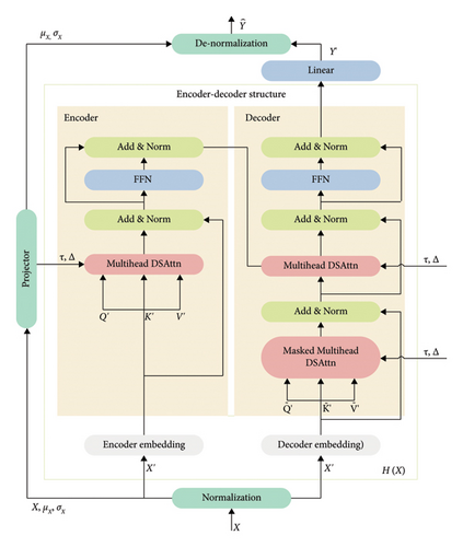
NSFormer enhances Transformer architecture by incorporating the series stationarization with two complementary operations as depicted in Section 2.2: (1) Series stationarization, which aims to mitigate the nonstationarity in the input of historical bridge structural response data, and (2) de-stationary attention (DSAttn), designed to reintegrate the nonstationary information from the input data. In alignment with Transformer [14], NSFormer employs the standard encoder-decoder architecture, as depicted in Figure 1. The encoder and decoder embedding incorporate both data and positional embeddings as inputs to the encoder and decoder, respectively, as presented in Section 2.3. The encoder is tasked with extracting features from historical bridge structural response data X, while the decoder is designed to predict the future response data , as described in Section 2.4.
2.2. Series Stationarization
As shown in Figure 1, the series stationarization is incorporated at both the input and output of NSFormer. This process comprises two corresponding operations: a normalization performed on the model input to address the nonstationarity of the series resulting from varying means and standard deviations, and a de-normalization performed on the output to revert the model outputs to their original statistical properties.
2.2.1. Normalization
2.2.2. De-Normalization
2.3. Encoder and Decoder Embedding
2.4. Encoder-Decoder Structure
The encoder consists of two encoder layers, each containing two main components: (1) Multihead DSAttn uses the normalized input and the statistics from normalization to estimate the attention that would have been derived from the original non-normalized input. Particularly, it employs 8-head DSAttn, accepting input without masks and parameters like the dropout rate, allowing flexible modulation of the attention distribution. (2) Feed-Forward Network (FFN) is a position-wise fully connected network. It applies the same transformation to each input position independently, further extracting features. Each encoder layer also includes residual connections and layer normalization (Add & Norm). Residual connections help gradients propagate more effectively, mitigating the vanishing gradient problem. The layer normalization stabilizes the training process by normalizing the activations of each layer.
The decoder includes the following three main components: (1) Masked Multihead DSAttn is similar to the multihead DSAttn in the encoder, but with the addition of a mask to ensure that when making prediction, only the data before it is visible, thus simulating the real-world bridge response prediction process. (2) Multihead DSAttn allows the decoder to focus on the output of the encoder, thereby obtaining information from the entire input sequence to assist in the generation of the current position. (3) FFN is similar as that in the encoder. It is used to extract further features. The decoder also includes Add & Norm to enhance the model’s stability and gradient propagation efficiency, and obtains the predictions by a linear layer finally.
2.4.1. DSAttn
2.4.2. Multihead DSAttn
2.4.3. FFN
2.5. Evaluation Metrics
3. Experiments
We conduct extensive experiments to evaluate the performance of NSFormer for the task of bridge structural response prediction on real-world datasets.
3.1. Experiment Settings
3.1.1. Data Description
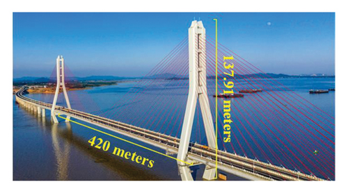
In this work, two types of data are collected from a double-tower cable-stayed bridge, Poyang Lake Second Bridge, the bridge bore arrangement is 790 meters, and the tower heights are 137.91 meters, as shown in Figure 2, in Jiangxi Province, China. The time spans a continuous period of 81 days from October 12, 2019, to December 31, 2019.
3.1.1.1. Deflection Dataset
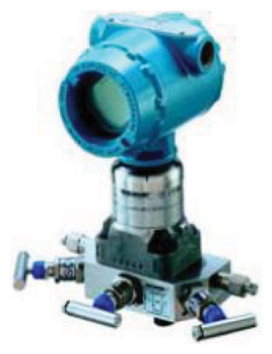
The bridge deflection is affected by multiple factors, including temperature variations, vehicle loads, wind loads, and support settlements. To measure the main girder deflection accurately, pressure transmitters based on the principle of communicating pipes are employed. The pressure transmitters selected have a range of ±250 in H2O, suitable for field test conditions. Specifically, Rosemount 3051C differential pressure transmitters are used as shown in Figure 3, and Table 1 summarizes their key specifications. The layout of the pressure transmitter sensors is illustrated in Figure 4, with all sensors installed on the maintenance walkway surface.
| Technical parameter | Model 3051C |
|---|---|
| Range | ±250 in H2O |
| Accuracy | 0.04% |
| Signal output | 4–20 mA |


The flow direction of water on the bridge is from west to east. Data acquisition is performed using the ADAM4117 module, which collects pressure data and outputs a 4–20 mA current signal. Data transmission uses the RS485 serial communication protocol. The client initiates data collection commands, and data are transmitted via a serial port server through an Ethernet switch to the collection client. The sampling frequency is set at 1 Hz. Displacement values at measurement points are derived by linearly transforming current signals, with upward displacement defined as positive. Among 13 measurement points, HS003-01 and HS107-02 serve as reference points with zero deflection. Therefore, deflection data from 11 sensor points are included in the dataset. The original sampling frequency is 1 Hz, and the deflection changes within 1 s are relatively small, and there are outlier and missing values due to some uncertain factors. Thus, we preprocessed the data as follows: first, we downsampled the data, taking an average value every second and interpolating any missing values. Then, we applied a 2-min rolling average to a specific sensor column. Next, we upsampled the data again, taking one record every 2 min, resulting in a final dataset with a total of 58,321 records. Note that we calculated the Z-scores for the deflection data of each sensor to identify outliers. If the Z-score exceeds 3 times of standard deviations, the original value is replaced with the average.
3.1.1.2. Strain Dataset
Strain measurements are obtained using BGK-4000 vibrating wire strain gauges coupled with BGK-Micro-40 automated data acquisition units to monitor stress and strain on the bridge structure. The BGK-4000 strain gauges, designed for steel and concrete structures, have a thermal expansion coefficient closely matching that of steel and concrete, minimizing temperature compensation requirements. Made of stainless steel, these gauges provide high precision, sensitivity, waterproofing, corrosion resistance, and long-term stability. Table 2 lists their main specifications and Figure 5 illustrates the strain gauge structure.
| Parameter | Specification |
|---|---|
| Standard range | 300 με |
| Nonlinearity | Linear: ≤ 1% FS; polynomial: ≤ 0.1% FS |
| Sensitivity | 1 με |
| Temperature range | −20 to +80°C |

The strain dataset includes data from 71 gauges distributed across 10 sections of the bridge (Figure 6): Sections 1–4 are bearing sections, six to nine are steel main girder sections, and 10-11 are bridge tower sections. Data are collected via the Micro-40 acquisition module, transmitted through RS485 protocol, a serial port server, and an Ethernet switch. Data collection occurs every 5 s. Two sensors showed abnormal data and were excluded. According to the characteristics of the sensor monitoring, the strain gauges are grouped into four subsets for analysis: 69 valid gauges (Strain-All), 34 steel main girder gauges (Strain-Main), 20 bearing gauges (Strain-Bear), and 15 bridge tower gauges (Strain-Tower). Since the strain gauge data is collected by multiple acquisition modules sequentially, with each module collecting data from different channels at different times and with inconsistent intervals, the sampling frequency of the strain data is inconsistent. To regularize the irregular time series, linear interpolation is employed. The basic idea is to find the two closest timestamps to each resample point (every 5 min) and interpolate. Additionally, to reduce the impact of abnormal fluctuations in the strain gauge data on the results, threshold elimination based on Z-scores is applied to each sensor data set, with the threshold set at three standard deviations. Following this processing, the strain dataset comprises a total of 23,329 records.

3.1.2. Baselines
- •
LSTM [18], a variant of RNN, is known for its ability to handle temporal dependencies and uses gating mechanisms. It is commonly used as a baseline model for sequential data processing.
- •
Transformer [14] is an encoder-decoder architecture, where both the encoder and decoder are featuring self-attention mechanisms, and multihead attention mechanisms.
3.1.3. Implementations
The experiments were implemented in Python based on an open-source deep learning framework PyTorch 1.7.1. All experiments were conducted on a machine equipped with an NVIDIA GeForce RTX 4070 Ti GPU and an AMD 5900X CPU. For LSTM, the following hyperparameters were used: 2 LSTM units with 64 hidden units, a dropout rate of 0.1, a learning rate of 0.001. The Transformer architecture consists of two encoder layers and one decoder layer. The hyperparameters for the Transformer include 8 self-attention heads with 512 hidden units and a dropout rate of 0.1, an FFN with 2048 hidden units. NSFormer retains the basic Transformer framework but replaces the standard self-attention mechanism with DSAttn, designed to handle nonstationary sequences with varying means and standard deviations. To ensure a fair comparison, all other settings in NSFormer keep consistent with Transformer. In the experiments, each dataset is split into three parts: 70% for training, 10% for validation, and 20% for testing the model performance.
3.2. Experimental Results
3.2.1. Overall Comparison
Table 3 presents an overall performance comparison of three models (i.e., LSTM, Transformer and NSFormer) across different datasets (i.e., Deflection, Strain-All, Strain-Main, Strain-Bear, Strain-Tower) and prediction horizons (6, 12, 24), using metrics MAE, RMSE, and MAPE. There are three main characteristics: (1) Firstly, LSTM shows consistent performance but with higher error rates. For example, MAE, RMSE, and MAPE values on Deflection dataset remain constant at 2.13, 2.78-2.79, and 0.16 respectively. This consistency suggests stability but indicates relatively high errors compared to Transformer and NSFormer, due to its limitations in handling long-term temporal dependencies compared to the attention-based mechanisms in the other models. (2) Moreover, Transformer shows moderate performance improvements over LSTM but is generally less accurate than NSFormer. Also, there is a slight increase as prediction horizons increase, indicating potential challenges in maintaining accuracy over larger horizons. As Transformer uses self-attention mechanisms to weigh the importance of different parts of the input sequence, it allows to capture global temporal dependencies more effectively than LSTM. (3) NSFormer consistently outperforms the other models across all datasets and prediction horizons, achieving the highest accuracy. For example, for a 24-step prediction horizon, NSFormer achieves MAE reductions of at least 22.88% for Deflection dataset (0.91 vs. 2.13 for LSTM and 1.18 for Transformer) and at least 66.67% for Strain-All dataset (0.71 vs. 3.05 for LSTM and 2.13 for Transformer), with similar improvements in terms of RMSE and MAPE. Although errors increase slightly with the prediction horizons getting larger, NSFormer maintains better accuracy than the other models. This suggests the effectiveness of its DSAttn in handling nonstationary patterns typical in bridge structural response prediction.
| Dataset | Model | LSTM | Transformer | NSFormer | ||||||
|---|---|---|---|---|---|---|---|---|---|---|
| Horizons | 6 | 12 | 24 | 6 | 12 | 24 | 6 | 12 | 24 | |
| Deflection | MAE | 2.13 | 2.13 | 2.13 | 0.95 | 1.03 | 1.18 | 0.65 | 0.75 | 0.91 |
| RMSE | 2.78 | 2.79 | 2.79 | 1.44 | 1.56 | 1.81 | 1.04 | 1.21 | 1.52 | |
| MAPE | 0.16 | 0.16 | 0.16 | 0.08 | 0.09 | 0.10 | 0.06 | 0.07 | 0.08 | |
| Strain-All | MAE | 3.05 | 3.05 | 3.05 | 2.02 | 2.05 | 2.13 | 0.5 | 0.57 | 0.71 |
| RMSE | 4.10 | 4.10 | 4.10 | 3.01 | 3.05 | 3.13 | 1.09 | 1.2 | 1.42 | |
| MAPE | 3.08 | 3.08 | 3.09 | 2.6 | 2.63 | 2.70 | 1.13 | 1.29 | 1.55 | |
| Strain-Main | MAE | 1.73 | 1.73 | 1.73 | 0.98 | 1.04 | 1.16 | 0.64 | 0.73 | 0.9 |
| RMSE | 2.38 | 2.38 | 2.39 | 1.58 | 1.66 | 1.82 | 1.28 | 1.39 | 1.61 | |
| MAPE | 2.64 | 2.64 | 2.64 | 2.46 | 2.51 | 2.6 | 1.63 | 1.83 | 2.19 | |
| Strain-Bear | MAE | 3.37 | 3.37 | 3.37 | 1.56 | 1.62 | 1.76 | 0.41 | 0.51 | 0.67 |
| RMSE | 4.27 | 4.27 | 4.27 | 2.13 | 2.23 | 2.45 | 0.95 | 1.13 | 1.43 | |
| MAPE | 1.84 | 1.84 | 1.84 | 1.02 | 1.09 | 1.26 | 0.54 | 0.66 | 0.83 | |
| Strain-Tower | MAE | 3.15 | 3.15 | 3.16 | 1.57 | 1.6 | 1.67 | 0.16 | 0.19 | 0.25 |
| RMSE | 4.64 | 4.64 | 4.64 | 2.2 | 2.24 | 2.32 | 0.46 | 0.51 | 0.58 | |
| MAPE | 1.51 | 1.52 | 1.58 | 0.84 | 0.87 | 0.96 | 0.43 | 0.46 | 0.51 | |
- Note: The bold values indicate the best performance for each metric (MAE, RMSE, and MAPE) across different models and horizons.
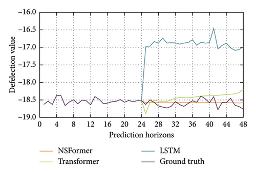
Besides, Figure 7 compares the deflection predictions of NSFormer, Transformer, and the ground truth for a case study. NSFormer closely aligns with the ground truth across all time steps, demonstrating its superior ability to capture temporal dependencies and nonstationary patterns in the data. In contrast, Transformer exhibits significant deviations from the ground truth, particularly in larger prediction horizons, where its predictions diverge substantially. This discrepancy highlights the limitations of standard Transformer in handling nonstationary data effectively over prediction horizons. NSFormer is attributed to its DSAttn mechanism, which dynamically adapts to changing data distributions, ensuring more accurate and stable predictions. Overall, NSFormer demonstrates significant advantages in predicting bridge responses by leveraging its ability to model nonstationary data (e.g., both deflection and strain data) effectively. This makes it particularly suitable for applications in SHM, where environmental and operational variability often induces nonstationary behaviors in bridge response data.
3.2.2. The Influence of Prediction Horizons
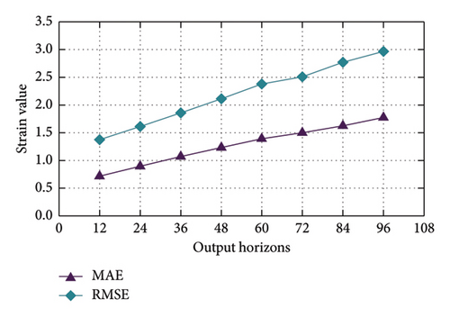
Figure 8 illustrates the performance of NSFormer on Deflection and Strain-Main datasets with fixed input horizons 24 and varying prediction horizons from 12 to 96, as measured by MAE and RMSE. In both datasets, the two metrics exhibit an increasing trend as the prediction horizon gets large, indicating a decline in predictive accuracy over larger horizons. For Deflection dataset (Figure 8(a)), RMSE consistently remains higher than MAE, with both metrics showing a gradual rise. A similar pattern is observed in Strain-Main dataset (Figure 8(b)), where RMSE again surpasses MAE across all horizons. The consistent gap between RMSE and MAE suggests that larger prediction errors contribute significantly to the overall error. Additionally, the rate of increase in errors is comparable between the two datasets, highlighting the challenges of long-term predictions for both.

3.2.3. The Influence of Input Horizons
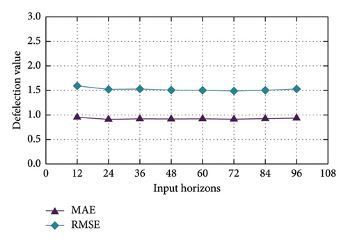
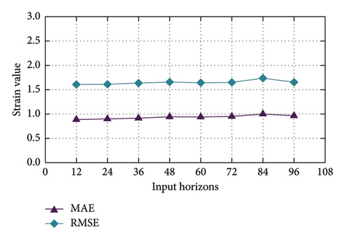
Figure 9 illustrates the prediction accuracy on varying input horizons from 12 to 96 and fixed prediction horizons 24, for Deflection and Strain-Main datasets. From the figure, it is easy to observe that the two metrics remain relatively stable across different input horizons, with only minor fluctuations observed. For Deflection dataset, both MAE and RMSE maintain low values, indicating that NSFormer effectively captures temporal dependencies regardless of input horizons. Similarly, in Strain-Main dataset, the model demonstrates consistent performance across all input horizons, with slightly higher error values compared to Deflection dataset due to the inherent complexity of strain data. This stability can be attributed to the DSAttn mechanism in NSFormer, which handles nonstationary data by dynamically adapting to changing temporal patterns. By effectively isolating and reintegrating nonstationary components, NSFormer maintains robust predictive accuracy across varying input horizons, making it particularly suitable for SHM applications where data variability is common.
4. Discussions
4.1. Comparative Analysis With Conventional Methods
Traditional models for bridge structural response prediction, such as LSTMs and Transformers, each have distinct strengths and limitations. LSTMs are effective at capturing temporal dependencies in sequential data due to their memory cell architecture, but they process data sequentially, which limits training efficiency and scalability. They also tend to focus on short-term dependencies and may struggle with long-range patterns, especially in highly nonstationary environments. Standard Transformers address some of these issues by leveraging self-attention mechanisms that allow parallel processing and improved modeling of long-range dependencies. However, standard Transformers assume stationarity in the input data, which can lead to suboptimal performance when faced with the nonstationary characteristics typical of SHM data.
The key novelty of our work lies in the introduction and application of NSFormer to bridge structural response prediction—a first in this domain. NSFormer incorporates the DSAttn mechanism, which explicitly models and adapts to the evolving statistical properties of real-world bridge structural response data. Unlike standard Transformers, NSFormer dynamically restores intrinsic nonstationary information within the attention mechanism, allowing it to maintain high predictive accuracy even as the data distribution shifts due to environmental or operational factors. Our comparative experiments demonstrate that NSFormer consistently achieves at 20% improvement in predictive accuracy over both standard Transformer and LSTM models across multiple nonstationary datasets. This superior performance underscores the model’s unique capability to handle the complex, time-varying nature of real bridge structural response data, which is a significant advancement over previous models. The main advantage of NSFormer is its robustness to nonstationary time series, which is critical for accurate and reliable bridge monitoring. It offers improved predictive accuracy, stability across varying input horizons, and the ability to capture complex temporal dynamics. However, like other deep learning models, NSFormer requires substantial computational resources for training and may experience reduced performance for long-term forecasting, where uncertainty and error propagation are more significant. Additionally, the interpretability of deep learning models remains a challenge compared to some traditional statistical approaches.
4.2. Practical Implications for SHM
The practical impact of adopting NSFormer in SHM is substantial. Reliable and accurate prediction of bridge responses enables more effective condition assessment, early detection of anomalies, and optimized maintenance scheduling. By leveraging real-time sensor data and advanced machine learning, stakeholders can shift from reactive to proactive maintenance strategies, reducing repair costs, minimizing downtime, and enhancing bridge safety and longevity. The demonstrated ability of NSFormer to address nonstationarity in bridge structural response data directly supports these practical benefits, as it ensures more robust and trustworthy predictions under real-world, variable conditions. The integration of NSFormer into SHM systems can also facilitate automated alerting and decision support, empowering engineers to make informed interventions based on data-driven insights.
5. Conclusions
This study presents the NSFormer as an effective approach for predicting bridge structural responses under varying operational and environmental conditions. By addressing the challenges of nonstationary data through its DSAttn mechanism, NSFormer achieves substantial improvements in predictive accuracy compared to traditional models, as validated on observed deflection and strain data from the Poyang Lake Second Bridge. The model’s robustness across diverse datasets and input horizons highlights its practical applicability for SHM systems, supporting more reliable and timely bridge condition assessments.
To further enhance the capabilities of NSFormer and broaden its impact, future research should focus on several key directions. First, extending the model to improve long-term prediction accuracy beyond current prediction horizons is critical, potentially through integrating hybrid architectures or advanced temporal regularization techniques. Second, incorporating additional heterogeneous data sources, such as environmental factors, traffic loads, and sensor fusion from multimodal measurements, could improve model robustness and generalizability under complex operational scenarios. Third, exploring the integration of NSFormer with emerging SHM frameworks, including Building Information Modeling and Internet of Things platforms, would enable automated, real-time monitoring and decision support, enhancing infrastructure management workflows. Finally, investigating explainability and uncertainty quantification within NSFormer predictions can provide valuable insights for engineers and stakeholders, fostering trust and facilitating risk-informed maintenance strategies.
In summary, NSFormer represents a significant advancement in bridge structure response prediction, offering a promising pathway toward smarter, safer, and more resilient infrastructure management. Continued interdisciplinary efforts combining machine learning innovations with domain-specific knowledge will be vital to fully realize the potential of artificial intelligence-driven SHM systems in civil engineering practice.
Conflicts of Interest
The authors declare no conflicts of interest.
Funding
This work was supported by the Young Scientists Fund of the National Natural Science Foundation of China (No. 62202018).
Open Research
Data Availability Statement
The data that support the findings of this study are available from the corresponding author upon reasonable request.


