Structural Control and Health Monitoring

Volume 2025, Issue 1 6558932

Research Article

Open Access

Predictive Model for Estimating the Weight of Existing RC Buildings Using Easily Accessible Structural Parameters

Jing Xu,

Jing Xu

orcid.org/0009-0003-5818-2409

College of Civil Engineering , Tongji University , Shanghai , 200092 , China , tongji.edu.cn

Search for more papers by this author

Kawsu Jitteh,

Kawsu Jitteh

College of Civil Engineering , Tongji University , Shanghai , 200092 , China , tongji.edu.cn

Search for more papers by this author

Yang Li,

Yang Li

orcid.org/0009-0006-0720-469X

College of Civil Engineering , Tongji University , Shanghai , 200092 , China , tongji.edu.cn

Search for more papers by this author

Jun Chen,

Corresponding Author

Jun Chen

[email protected]

orcid.org/0000-0002-6025-418X

College of Civil Engineering , Tongji University , Shanghai , 200092 , China , tongji.edu.cn

State Key Laboratory of Disaster Reduction in Civil Engineering , Tongji University , Shanghai , 200092 , China , tongji.edu.cn

Search for more papers by this author

Jing Xu,

Jing Xu

orcid.org/0009-0003-5818-2409

College of Civil Engineering , Tongji University , Shanghai , 200092 , China , tongji.edu.cn

Search for more papers by this author

Kawsu Jitteh,

Kawsu Jitteh

College of Civil Engineering , Tongji University , Shanghai , 200092 , China , tongji.edu.cn

Search for more papers by this author

Yang Li,

Yang Li

orcid.org/0009-0006-0720-469X

College of Civil Engineering , Tongji University , Shanghai , 200092 , China , tongji.edu.cn

Search for more papers by this author

Jun Chen,

Corresponding Author

Jun Chen

[email protected]

orcid.org/0000-0002-6025-418X

College of Civil Engineering , Tongji University , Shanghai , 200092 , China , tongji.edu.cn

State Key Laboratory of Disaster Reduction in Civil Engineering , Tongji University , Shanghai , 200092 , China , tongji.edu.cn

Search for more papers by this author

First published: 13 July 2025

https://doi.org/10.1155/stc/6558932

Academic Editor: Francesc Pozo

Share a link

Email
Wechat
Bluesky

Abstract

The weight of existing buildings is a critical parameter in various structural engineering applications, including seismic assessment, uneven settlement evaluation, structural vibration control, building relocation, and demolition operations. While current practice typically estimates this value by multiplying floor area multiplied by an empirical unit weight coefficient. This approach faces limitations when the original design details are unavailable, making total floor area difficult to determine. To address this challenge, this study develops predictive models for estimating the weight of existing reinforce concrete (RC) buildings using easily accessible structural parameters, such as structural height, plan dimensions, number of stories, and fundamental period. A database comprising the weights and related design parameters of 732 RC buildings was developed through an extensive literature search. The maximum information coefficient and Kruskal–Wallis analysis of variance were used to identify factors that significantly influence building weight. Subsequently, regression formulas for building weight, incorporating structural height, plan dimensions of a standard floor, fundamental period, and structural type were established. These prediction formulas were applied to five building examples, and the results were compared with actual values. The comparison shows that the weight prediction formulas have good accuracy and can be used in state assessment of existing buildings and parametric modeling in disaster prevention analysis of urban buildings. Finally, the predictive models have been deployed on an online web page for the convenience of users.

1. Introduction

Weight, like height, is a very important structural characteristic of a building, yet it rarely receives the attention of design engineers and researchers. Taking the prevalent structural type [1]—reinforced concrete (RC) structures—as a prime example, the significance of building weights becomes even more evident when analyzed on both the individual building scale and the urban building cluster scale.

On the individual building scale, the weight of a new building is the core parameter in many design tasks such as determining the amplitude of seismic load, comparing the performance of different structural systems, selecting proper foundation types, and evaluating the total construction project cost. For a completed RC building, its weight is also a decisive factor in tasks such as seismic vulnerability analysis [2], structural health monitoring and vibration control [3, 4], uneven settlement assessment, building moving, and demolition.

On the urban building cluster scale, when conducting urban seismic resilience analysis (currently a hot research topic in civil engineering), a crucial step involves swiftly and precisely developing parametric models for a substantial number of RC buildings within the targeted region [5–7]. This process requires the weight of each building as a prerequisite in order to determine other structural parameters as stiffness and frequency [8]. Furthermore, the building’s weight serves as a pivotal metric in evaluating the transformation of building material stock within the urban planning area, contributing to the assessment of ecological sustainability within the conservation and regeneration design framework of old city revitalization projects [9, 10]. Another interesting scenario is the assessment of city-scale ground subsidence [11] that is closely related to building weights.

Despite the significant importance highlighted above, there is still no reasonable and accurate model available for predicting structural weight. In current engineering practice, the weight of a building W is mainly obtained in two ways: (1) For a new building or an existing building with relevant original design drawings/numerical models, its weight (representative value) is normally calculated as W = D + L or W = D + 0.5 L [12], where D is the total dead load and L is the total live load. Specifically, the dead load D can be, and generally is calculated by the dimensions and material densities of all the structural members, and the live load L can be estimated by the total floor area times the live load value as specified in a corresponding design guideline; (2) for an existing building without its original design details, the weight is usually estimated using an empirical equation as W = S × P, where S is the total floor area and P is a coefficient representing the weight per unit area. Estimating the floor area S in this scenario is challenging due to the limited information available. Additionally, the coefficient P is an empirical value that varies considerably for different buildings. For example, it is mentioned in China’s “Technical Specification for Concrete Structures of Tall Buildings (JGJ3-2010)” [13] that the weight of reinforced concrete high-rise frame and frame-shear wall (F-SW) structures is about 12–14 kN/m², and that of SW and tube structures is about 13–16 kN/m². The above empirical value P includes self-weight (dead load) that counts for 75%–80% and live load that accounts for 25%–20%. It is also given in the “National Technical Measures for Design of Civil Construction: Structure” [14] that P = 6–8 kN/m² for steel structures, 9–12 kN/m² for multistorey masonry buildings, and 14–16 kN/m² for RC high-rise buildings. There are also different suggested values in different literature and books, and these empirical values differ in amplitude, range of variation, range of application, data sources and so on. Consequently, employing varying values of P to assess the weight of a RC building can potentially introduce a margin of error ranging from 15% to 30% or even greater.

Given the crucial importance of accurately predicting the weight of RC buildings, it is surprising to find a lack of relevant research in this area. Some studies, although only loosely related, have focused on the weight of construction materials or structural components. For instance, Aghayere and Vigil [15] listed the typical weights for wood framing, roof trusses and floor joists in their book. Wang and Tsavdaridis [16] proposed a minimum-weight design method for modular building systems, yet they did not address how to predict the overall weight of a modular building. Jefferson and Tatiana [17] conducted a statistical study on the Specific Total Weight (STW) of 40 Andean residential buildings in Ecuador, built between 1980 and 2020. The results showed that the overall STW of buildings increased by a relatively small margin (only 1.36 times). Parsons [18] explored a very interesting topic: the weight of cities. In the study, the weight of buildings was calculated by using the planar dimensions and heights of each building, obtained through GPS technology, combined with empirical weight coefficients. This was then used to estimate the weight of the city. The paper also noted that, due to the presence of numerous assumptions, the method for calculating building weights is quite rough, which is the main source of error in calculating the weight of the city. The literature review also indicates that there are currently no available models for predicting the weight of RC buildings.

To address above issues, this study proposes models for predicting the weight of RC buildings using easily obtainable structural parameters such as area, height, plan dimensions, construction materials, and natural period, either individually or in combination. These predictive models are developed by fitting a large dataset of actual structural weight data. The development process is presented as follows: Section 2 establishes the RC building weight database through an extensive literature review and explains the data collection sources and selection of data characteristics. Section 3 analyzes the correlation between various structural parameters and building weight using nonparametric exploratory methods. Section 4 uses the highly correlated parameters as independent variables to fit the database and establish the weight prediction equations. Section 5 employs case analysis to verify the applicability and accuracy of the proposed prediction models by comparing the predicted weights with the actual values. For ease of use, Section 6 deploys the prediction models on a public webpage, where users can input several key parameters to predict building weight. Finally, Section 7 summarizes the main findings of this study along with its limitations.

2. RC Building’s Weight Database

2.1. Development of the Database

By collecting building design data from design institutes, literature, and books, this study has compiled a database of weight values and corresponding design parameters for 732 RC buildings constructed in China since 2010. To ensure the representativeness of the data, all the data records in the database are from real design projects, and those examples for structural models and theoretical analysis purpose have been excluded. Moreover, considering the significant differences in live load levels and component sizes, the database only includes RC structures such as residential buildings and standard office buildings, excluding structures like libraries, archives, and large public buildings.

Each building corresponds to a data record, which includes the following characteristics: building weight, main structural material, lateral-force resisting system (LFRS), above ground floor area, height, number of storeys, name, fundamental period, site category, and seismic precautionary intensity. The first five parameters (up to height) are mandatory, while the last five parameters can be optional. It is necessary to clearly specify that the ‘building weight’ in this database refers to the dead load of the building plus 0.5 times the live load, that is, W = D + 0.5 L, which the representative value of the building weight as defined by Chinese design codes. A reduction coefficient 0.5 for live load is adopted to account for the very low probability of full live load on all floors of a building. Meanwhile, height refers to the height from the ground to the main roof, that is, the structural height, excluding the height of local protrusions. The fundamental period refers to the first (lowest) translational vibration period of the structure.

2.2. Statistics of the Database

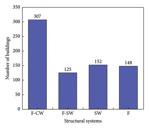
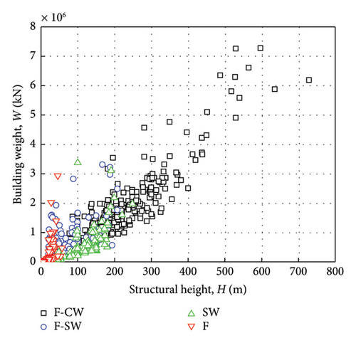
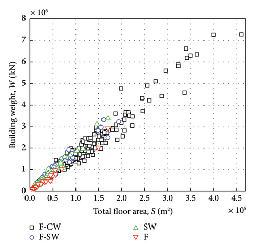
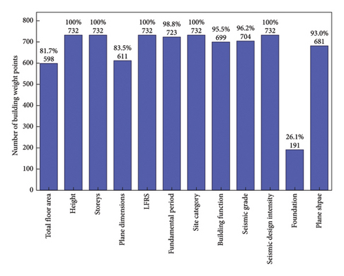
The RC buildings in the database contain four structural systems: F-core wall (F-CW), F-SW, SW, and F structures, the amount of data for each system is shown in Figure 1. Figure 2 further categorizes the database samples by structural systems and shows the distribution of total building weight with structural height and total floor area. It can be seen that the building weight is positively correlated with structural height and floor area. The total floor area in the database ranges from 66 to 460,700 m², and the building weight ranges from 923 to 7,276,834 kN, with the average value of all the building weights being 785,479 kN. Figure 3 shows the number and ratio of records in the database for certain factor; for example, 732 records (100%) for height, 598 records (81.69%) for total floor area, and 191 (26.09%) for foundation.

Details are in the caption following the image — **Figure 1**
Open in figure viewer PowerPoint

Number distribution of buildings with different structural systems.

3. Correlation Analysis of Influencing Factors and Building Weight

There are many factors that can affect the weight of a building, such as floor area, structural height, material, structural system, etc. Quantifying the correlation degree between each factor and building weight is important for the subsequent development of regression prediction models. Preanalysis shows that the data under most categories do not follow the normal distribution. Therefore, in this study, we employ two nonparametric methods, which impose no stringent constraints on the distribution type or homogeneous variance of the data, to assess the correlation between individual factors and the building weight. In particular, the maximal information coefficient (MIC) is used to assess numerical parameters (such as height or area), and the Kruskal–Wallis one-way ANOVA (K-W ANOVA) is adopted to evaluate categorical variables (such as LFRS and building function).

3.1. MIC Analysis

MIC was proposed by Reshef et al. [19] in 2011 and has since been widely used in big data analysis and data mining. It evolved from the mutual information theory, in which mutual information represents the amount of information about another random variable contained in a given random variable, or the extent to which the uncertainty of another random variable is reduced when a given random variable is known. For random variables U and V, the mutual information is calculated as follows:

()

where MI(U; V) represents the mutual information between U and V, p(u, v) is the joint probability density distribution function of the two random variables, and p(u) and p(v) are their marginal probability density distribution functions, respectively.

Taking U and V as floor area and building weight; for example, the MIC of them is calculated in the following three main steps.

1.
The paired dataset of D(U, V) is discretized on a two-dimensional plane on which an x-by-y grid can be divided to encapsulate all sample points. Each grid is assigned a probability equal to the number of sample points within the grid divided by the total number of paired samples, thus obtaining the probability distribution D|_G of the dataset D(U, V) over the current grid partitioning method.
2.
When the number of grids is determined (i.e., fixed values of x and y), different gridding patterns of the dataset are obtained by changing the position of the grid lines. For each pattern, the mutual information MI(D|_G; x, y) is calculated by equation (2), and the maximum value of all the calculated results is taken as the representative mutual information for the given x-by-y configuration, which is denoted as
()
3.
The values of x and y are traversed to exhaust all possible data encapsulation schemes, and the representative mutual information MI^∗(D; x, y) corresponding to all partition configurations is calculated. Finally, MIC for U and V is the maximum value of all representative mutual information after normalization as shown in equation (3):
()
where n is the total number of samples. B(n) is the upper limit of the number of bins based on the maximum resolution of the computer, which implies that the product of the number of grids (x × y) in two orthogonal directions should be less than B(n).

MIC can effectively measure the correlation between two numerical variables, and its superiority over traditional methods is mainly reflected in the following three aspects: normalization, generality and equitability. Equation (3) shows that MIC is essentially normalized mutual information with a value range of [0, 1], which is close to the coefficient of determination R² between two numerical variables. Thus, the closer the coefficient is to 1, the more correlated the two parameters are. Generality means that MIC can effectively capture a large number of different kinds of correlations, including linear, nonlinear, monotonic, nonmonotonic, functional superposition, and even nonfunctional forms of correlation. Equitability implies that MIC can assign very close values to data with different functional forms but the same noise ratio [20].

The MIC between building weight and floor area (S), structural height (H), fundamental period (T), number of floors (N), plane length (L), plane width (B), standard floor area (L × B), and approximate area (N × L × B) have been calculated and listed in Table 1. For individual parameter, Table 1 shows that the MIC of S and building weight is the largest, followed by H, T, B, and N. For combined parameters, the approximate area (N × L × B) has a very high MIC value as 0.95, and the standard floor area (L × B) has a reasonable value as 0.60. The results in Table 1 indicate that the total area S is the most effective geometric parameter for establishing empirical formulas to predict building weight. Furthermore, since the parameters N, H, L, B, and T for existing buildings are generally easier to obtain accurately than the total area S, these parameters (either individually or in combination) will be utilized as regression variables in developing weight prediction models.

Table 1. MIC of building weight and different geometric parameters.

Geometric parameter	n	MIC
S	598	1.0000
H	732	0.6946
N	732	0.6270
L	611	0.3057
B	611	0.6565
T	723	0.6748
L × B	611	0.6063
N × L × B	611	0.9502

3.2. Kruskal–Wallis ANOVA

After selecting the numerical variables for the prediction model, it is essential to examine the impact of other semantic factors on building weight, such as LFRS, seismic precautionary intensity, site conditions, and building functions, which are not applicable to the MIC method. Consequently, the K-W ANOVA is employed to quantify the influence of categorical variables. K-W ANOVA is a nonparametric testing method that does not require samples to follow a specific distribution or exhibit homogeneity of variance. It assesses the significance of categorical variables based on the ranks of the samples, which represent the sequential positions of each sample when all samples are arranged in ascending order of their numerical values [21–23].

Five text-variable factors, including LFRS, site category, building function, seismic precautionary intensity, and seismic grade are tested by K-W ANOVA. The geometric parameter H is also checked for comparison. For each factor, the samples of building weight associated with it in the database are first divided into several groups. Specifically, LFRS is categorized into four groups as F-CW, F-SW, SW, and F; site category is categorized into Class I, II, III and IV; building function is categorized into office, hotel, commerce, residence, complex, factory, and school; seismic precautionary intensity is categorized into 6, 7, 7.5, and 8°; seismic grade is categorized into five groups: extra grade one, grade one, grade two, grade three and grade four. Finally, structural height H is divided into four groups: (0, 27] m, (27, 100] m, (100, 300] m, and above 300 m.

The application step of K-W ANOVA for each factor is to first mix multiple groups of samples together, determine the rank of each sample in the mixed dataset, then replace the original sample with the mixed rank, and sum the mixed rank of each group of samples. The greater the difference of average mixed rank in each group, the greater the difference between groups, indicating a stronger correlation. Therefore, the test quantity of K-W ANOVA can be expressed as

()

where n_j is the number of samples in group j, n is the total number of samples, and r_j is the sum of the mixed ranks of samples in group j (j = 1, 2, …, k).

Considering the usual presence of knots in groups, χ is further revised to χ_corr.

()

where τ_j is the length of knot j, and g is the total number of knots in all groups. Under the null hypothesis, χ_corr follows approximately the chi-square distribution with k − 1 degrees of freedom.

When the degrees of freedom k-1 are fixed, the larger χ_corr calculated by equation (5), the greater is the influence of the factor [24]. Due to the large sample size, underflow problems often occur in the p value calculation of K-W ANOVA. Therefore, the ratio of χ_corr to χ_crit is used in this study to represent the influence degree of each factor, where χ_crit is the critical value of the chi-square distribution at the 0.05 significance level. This method requires that the χ_crit of each influence factor be the same, which means that the number of groups under different influence factors should be equal to the extent possible. Thus, except for the building function (categorized into seven groups) and seismic grade (categorized into five groups), other factors are all categorized into four groups.

Table 2 shows results of K-W ANOVA test for the selected factors, where r_avg represents the mixed average rank of each group. At the significance level of 0.05, when the number of groups k = 4, the corresponding χ_crit = χ² (3; 0.95) = 7.815. Moreover, when k = 5, χ_crit = χ² (4; 0.95) = 9.488, and k = 7, χ_crit = χ² (6; 0.95) = 12.592. Table 2 shows the degree of influence of each factor on the building weight, in descending order, is H, LFRS, seismic grade, building function, site category, and seismic precautionary intensity. The result indicates that LFRS needs to be a categorical variable for developing weight prediction models. In addition, considering the limited amount of data currently collected, if the seismic grade is taken as another categorical variable, the amount of data in each category is relatively small, resulting in a decline in the accuracy and robustness of the prediction models. It is important to note that, although the text-variable factors selected in Table 2 are derived from specific Chinese codes [12, 13], they possess a certain degree of adaptability and generalizability, and can potentially be applied in different regional or regulatory contexts with appropriate conversions or modifications.

Table 2. Results of Kruskal–Wallis ANOVA for each factor.

Factor	Group no	Group feature	n	r_avg	χ_corr	χ_corr/χ_crit
H	1	0–27 m	163	102.67	524.87	67.16
	2	27–100 m	202	288.29
	3	100–300 m	321	502.80
	4	> 300 m	46	693.66

LFRS	1	F-CW	307	546.50	462.87	59.23
	2	F-SW	125	355.09
	3	SW	152	246.08
	4	F	148	126.44

Seismic grade	1	Extra grade	102	587.58	427.84	45.09
	2	Grade 1	263	466.92
	3	Grade 2	157	333.36
	4	Grade 3	132	142.20
	5	Grade 4	50	83.87

Building function	1	Office	228	403.93	303.58	24.11
	2	Hotel	30	395.03
	3	Commerce	61	177.91
	4	Residence	169	246.43
	5	Complex	151	581.55
	6	Factory	8	261.88
	7	School	52	222.77

Site category	1	Class I	5	405.80	86.02	11.01
	2	Class II	338	409.61
	3	Class III	242	392.86
	4	Class IV	147	222.64

Seismic design intensity	1	Intensity 6	163	351.31	11.83	1.51
	2	Intensity 7	399	384.91
	3	Intensity 7.5	55	286.24
	4	Intensity 8	115	362.53

4. Predictive Models of RC Building’s Weight

Based on the above correlation analysis result, geometric parameters S, H, N, L, B, and dynamic characteristics T are taken as independent variables, and LFRS is taken as classification variable to conduct regression analysis on the building weight.

4.1. Formulas of Weight and Total Floor Area

Assuming that the weight of a building is linearly related to its floor area, the form of the empirical formula is as follows:

()

where W is the total weight of the building (unit: kN), S is the total floor area (unit: m²), α₁ (kN/m²) and β₁ (kN) are the constant coefficients obtained by fitting different structural systems.

The weights of the four LFRS types are fitted by the least square method using equation (6), and the fitting effect is assessed by the coefficient of determination R². The closer is the value of R² to 1, the better is the fitting effect. The results of regression analysis are shown in Table 3, where n is the number of valid sample points.

Table 3. Unconstrained regression results of building weight and floor area.

LFRS	n	α₁	β₁ (× 10⁴)	R²
F-CW	231	16.846	−1.884	0.9505
F-SW	98	17.779	3.996	0.9631
SW	125	19.042	−1.648	0.9834
F	144	15.285	−0.527	0.9805

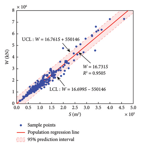
The R² of the four structural systems in Table 3 is all above 0.95, and the highest is 0.98, indicating a very good regression effect. It is also noted that the regression coefficient β₁ (i.e., the intercept) is about two orders of magnitude different from the average weight (7.85 × 10⁵ kN) of all buildings in the database. Therefore, in order to be consistent with the traditional estimation formula W = P × S for ease of use, as well as to satisfy the physical constraint that zero building area corresponds to zero building weight, regression is fitted again after the coefficient β₁ in equation (6) is set to zero. Finally, the results of the new constrained regression are shown in Table 4.

Table 4. Constrained regression results of building weight and floor area.

LFRS	n	α₁	R²
F-CW	231	16.731	0.9505
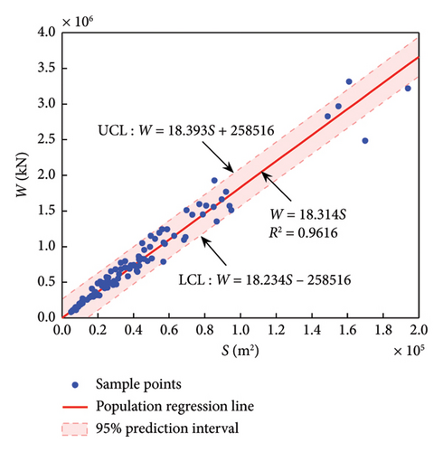
F-SW	98	18.314	0.9616
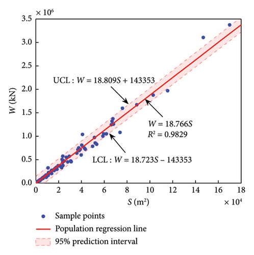
SW	125	18.766	0.9829
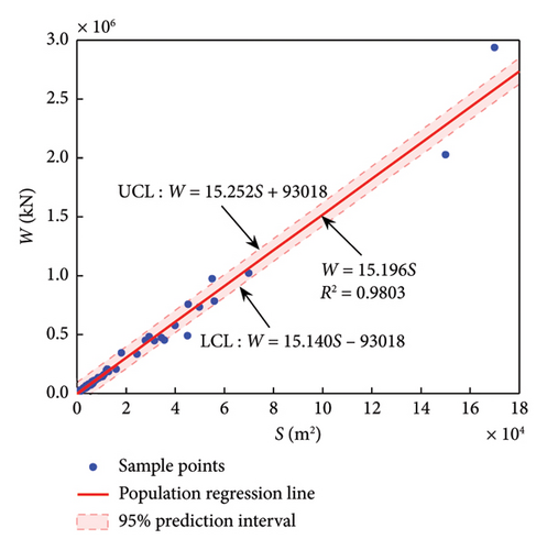
F	144	15.196	0.9803

Compared with Table 3, the change (decrease) of the coefficient of determination R² corresponding to each structural system in Table 4 is minimal, indicating that the regression effect is still very good. In addition, the coefficients α₁ of F-CW and SW are 16.73 and 18.77 kN/m², respectively, exceeding the upper limit of the recommended range of 13–16 kN/m² in the relevant specification [13]. Similarly, α₁ of F-SW and F are 18.31 and 15.20 kN/m², respectively, which are 30.8% and 8.6% larger than the upper limit of the corresponding recommended range of 12–14 kN/m² [13]. The above results indicate that the unit weight coefficient currently in use is relatively low.

The formulas in Table 4 reflect the variation trend of the sample median, and for practical application, it is also necessary to know their reasonable range. In this paper, two-sided 95% prediction interval is given, denoted as upper control limit (UCL) and lower CL (LCL) in following figures. A 95% prediction interval means that given the value of the independent variable, the value of the dependent variable has a 95% probability of falling within this interval. Finally, the prediction models with the overall regression line and reasonable intervals are shown in Figures 4(a), 4(b), 4(c), 4(d).

4.2. Formulas of Weight and Structural Height

Because the total area of the existing building is often difficult to accurately obtain, while the height is easier to obtain or measure, and the correlation coefficient between H and weight is above 0.9. Therefore, the following attempts to predict the building weight from the readily available structural height.

The commonly used formula for the fundamental period and height of a structure [25] is

()

where T is the fundamental period (unit: s).

If a building is regarded as a homogeneous cantilever column, its fundamental period can be expressed as

()

where m is the total mass (unit: kg), E is the elastic modulus of the material (unit: N/m²), and I is the moment of inertia of the section (unit: m⁴).

The fundamental period serves as a bridge to relate building weight and H. Combined with equations (7) and (8), the relationship between building weight and H can be symbolically expressed as equation (9) (in general form) and equation (10) (in logarithmic form).

()

where α₂, β₂, and γ are the coefficients to be fitted for different structural systems.

The regression analysis is carried out in the same way as in the previous section. The corresponding results are presented in Table 5, where the values in each column without brackets correspond to equation (9) and those with brackets correspond to equation (10). Obviously, for F-CW and F-SW, equation (9) corresponds to a higher coefficient of determination, while for SW and F, equation (10) corresponds to a higher coefficient of determination. The regression curves with higher R² of each structural system and their reasonable scopes are shown in Figure 5.

Table 5. Regression results of building weight and structural height.

LFRS	n	α₂	β₂	γ	R²
F-CW	307	665.443 (1.149)	297,374 (3.542)	1.422 (/)	0.8202 (0.7776)
F-SW	125	0.0486 (0.612)	561,079 (4.653)	3.254 (/)	0.3139 (0.2631)
SW	152	22.100 (1.492)	45,243 (2.588)	2.089 (/)	0.5823 (0.8892)
F	148	3192.64 (2.388)	−78125 (1.832)	1.452 (/)	0.3136 (0.8021)

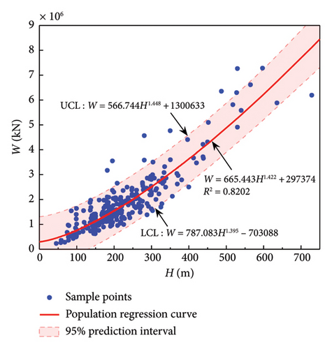
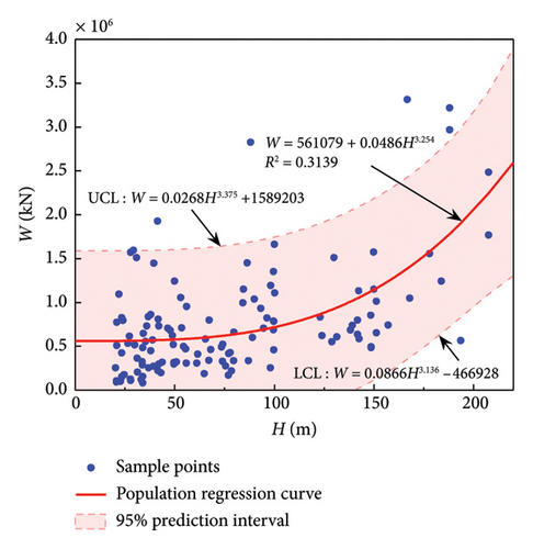
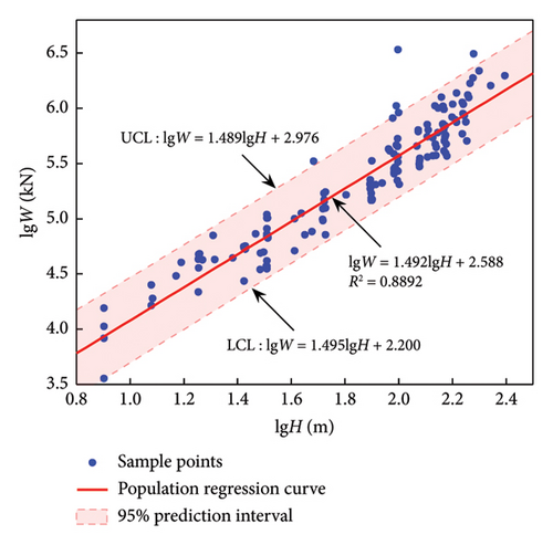
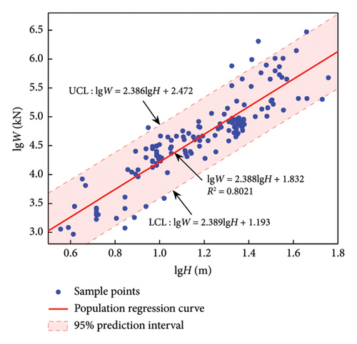
Table 5 shows that the R² of the three systems F-CW, SW, and F are all above 0.8, and the former two are above 0.82, indicating a good regression effect. Overall, due to the simplifications and assumptions in the above derivation process, the resulting prediction accuracy is lower than that based on floor area (Table 4), but these prediction formulas are also useful due to the fact that height is more readily available than area. Therefore, a modest trade-off in prediction accuracy is considered acceptable. For F-SW, no matter which regression formula, the highest R² is only 0.31. This is related to the flexible and diverse arrangement of SW in F-SW system [26], which is not directly related to the height of the structure. Therefore, height-dependent regression formula is not available for buildings with F-SW system.

4.3. Formulas of Building Weight and Multiple Variables N, L, and B

In the research of structural period prediction formulas, double geometric parameter regression analysis is also a common method. For example, the fundamental period empirical formula of RC SW structure is [27]. Inspired by this, this section uses multiple parameters for regression analysis of building weight, the core of which is to construct new combined regression variables using easily obtained structural parameters.

Considering that the total floor area can predict the weight well, the combined parameters of the plane dimensions and storeys are first tried as regression variables, and the specific regression form is as follows:

()

Note that equation (11) is a logarithmic equation whose general form will contain the product of NLB, related closely to the total area of the building. The regression results of equation (11) are listed in Table 6, and the corresponding predictive models are shown in Figure 6.

Table 6. Regression results of building weight and N, L, and B.

LFRS	n	α₃	α₄	β₃	R²
F-CW	257	1.051	0.511	2.756	0.8725
F-SW	92	0.919	0.777	2.049	0.8769
SW	129	1.070	0.871	1.456	0.9819
F	133	1.011	0.958	1.245	0.9908

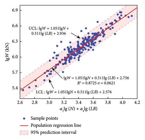
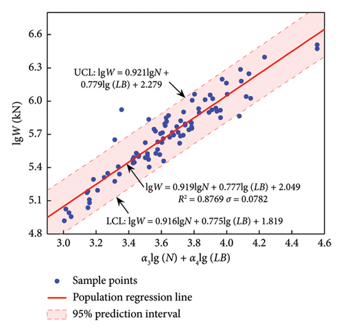
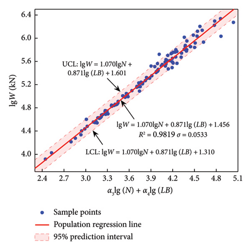
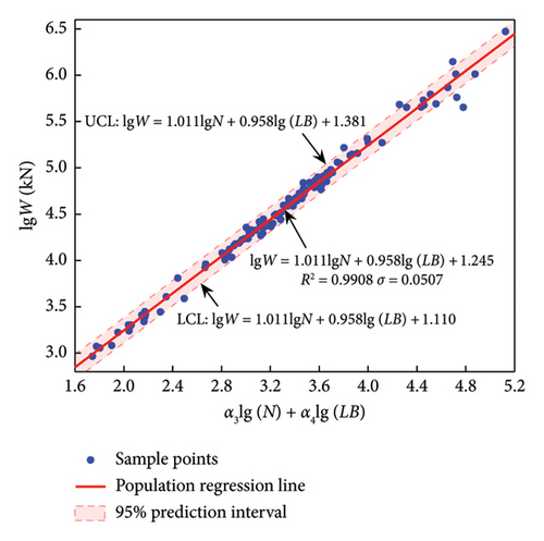
The results show that R² of the four structural systems are all above 0.87, and the R² of SW and F reach a high value (0.98), indicating a very good fit for this combination of parameters.

4.4. Formulas of Building Weight and N, L, T, and H

Fundamental period is the inherent dynamic characteristic of a structure, which can comprehensively reflect its stiffness and mass characteristics. For existing buildings, T can usually be measured more easily. Therefore, if the actual building is simplified as a cantilever column and the section is simplified as a rectangular plane, a relationship between weight and T, H, N, and L can be derived by combining equation (8), and the logarithmic coordinate form is

()

Equation (12) is applied to the data of the four structural systems, and the regression results obtained are listed in Table 7. The predictive models with empirical formulas and 95% confidence (prediction) intervals are presented in Figure 7.

Table 7. Regression results of building weight and N, L, T, H.

LFRS	n	α₅	α₆	α₇	α₈	β₄	R²
F-CW	257	0.614	0.579	0.632	0.136	2.836	0.8490
F-SW	92	1.178	1.268	−0.174	−0.061	1.463	0.8088
SW	129	2.086	0.870	−0.597	0.184	0.940	0.9756
F	133	1.219	1.308	0.279	0.058	0.858	0.9528

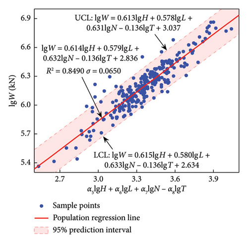
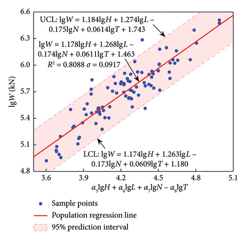
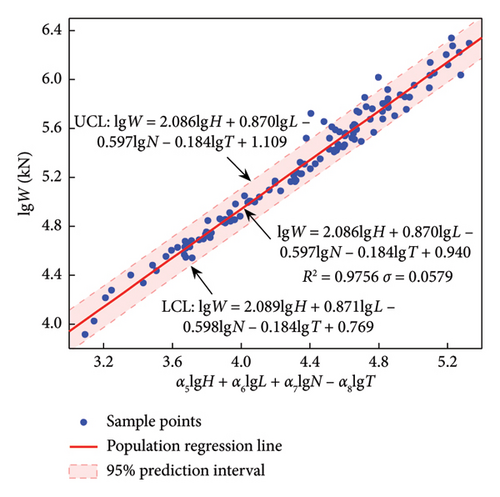
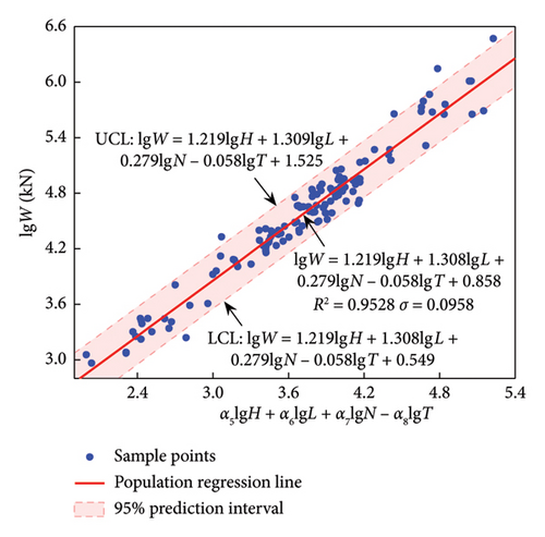
The results in Table 7 show that all R² exceeds 0.8, and the R² of SW and F exceed 0.92; indicating that the effect is good and relevant formulas can be used.

5. Weight Prediction Formulas and Application Examples

5.1. Summary of Prediction Formulas of Building Weight

Based on the above regression results, Table 8 summarizes the recommended prediction formulas for four kinds of RC building’s weight under different known conditions. In practical application, the corresponding weight prediction formulas can be selected according to the known parameters (S, H, L, B or T) of the specific structure. For description convenience, the prediction models using S, H, (NLB) and (NLTH) are named as Model 1 (M1) to Model 4 (M4), respectively. When more than one model is applicable (i.e., more parameters are available), the average of all predicted values can also be used as the weight representative value.

Table 8. Recommended prediction formulas for RC building’s weight.

LFRS	M1: S/m²	M2: H/m	M3: N, L/m, B/m	M4: N, L/m, H/m, T/s
F-CW	α₁ = 16.73	α₂ = 665.44 β₂ = 297,374 γ = 1.422	α₃ = 1.051 α₄ = 0.511 β₃ = 2.756	α₅ = 0.614 α₆ = 0.579 α₇ = 0.632 α₈ = 0.136 β₄ = 2.836

F-SW	α₁ = 18.31	NA	α₃ = 0.919 α₄ = 0.777 β₃ = 2.049	α₅ = 1.178 α₆ = 1.268 α₇ = −0.174 α₈ = −0.061 β₄ = 1.463

SW	α₁ = 18.77	= 1.492 = 2.588	α₃ = 1.070 α₄ = 0.871 β₃ = 1.456	α₅ = 2.086 α₆ = 0.870 α₇ = −0.597 α₈ = 0.184 β₄ = 0.940

F	α₁ = 15.20	= 2.388 = 1.832	α₃ = 1.011 α₄ = 0.958 β₃ = 1.245	α₅ = 1.219 α₆ = 1.308 α₇ = 0.279 α₈ = 0.058 β₄ = 0.858

Note: M1: W = α₁S, M2: W = α₂H^γ + β₂ or , M3: lg (W) = α₃ lg (N)+α₄ lg(LB) + β₃, M4: lg (W) = α₅ lg (H)+α₆ lg(L) + α₇ lg(N) − α₈ lg (T) + β₄.

5.2. Example I: Five Buildings

The above prediction models are applied to five engineering examples, covering four types of LFRS. Table 9 shows the main structural features and important design parameters of these examples. Note that all these buildings are located in China and are collected from recent literature, and are not included in the current database. Table 10 compares the predicted result with the true weight value (calculated by the design software or given in the literature), where the positive/negative deviation sign indicates the proportion of the predicted value greater/less than the true value. The last column in Table 10 is the estimation of the existing empirical model, which is 13 kN/m² (median of 12–14 kN/m²) for F and F-SW or 14.5 kN/m² (median of 13–16 kN/m²) for F-CW and SW multiplied by the total floor area [13].

Table 9. General information about five buildings.

Structural information	Building 1 (B1) [28]	Building 2 (B2) [29]	Building 3 (B3) [30]	Building 4 (B4)	Building 5 (B5)
Region	China	China	China	China	China
LFRS	F-CW	F-CW	F-SW	SW	F
Building function	Office	Complex	School	Residence	Commerce
Seismic intensity	8	7	7	7	7
Design PGA	0.20 g	0.10 g	0.15 g	0.15 g	0.10 g
Site category	III	III	III	III	II
Area (S/m²)	38,287	82,000	23,690	1947	1097
Floors (N)	23	36	9	7	2
Height (H/m)	84.1	156.3	40.05	21.15	9.65
L × B (m)	40.8 × 40.8	77.4 × 27.0	101.6 × 23.5	26.6 × 11.5	41.8 × 15
Building weight (W/kN)	617,338	1,350,289	419,946	35,420	15,870
Period (T/s)	1.798	4.304	0.860	0.651	0.320

Table 10. Prediction results of building weights (unit: kN).

LFRS	NO	Actual weight	M1	M2	M3	M4	Mean of M2–M4	Empirical
F-CW	B1	617,338	640,575	660,595	681,194	597,527	646,439	555,157
	B1	617,338	3.76%	7.01%	10.34%	−3.21%	4.71%	−10.07%
	B2	1,350,289	1,371,942	1,174,214	1,225,314	1,492,951	1,297,493	1,189,000
	B2	1,350,289	1.60%	−13.04%	−9.26%	10.56%	−3.91%	−11.95%

F-SW	B3	419,946	433,859	NA	356,927	531,578	444,253	307,970
F-SW	B3	419,946	3.31%	NA	−15.00%	26.58%	5.79%	−26.67%

SW	B4	35,420	36,538	36,759	33,512	29,785	33,352	28,232
SW	B4	35,420	3.16%	3.78%	−5.39%	−15.91%	−5.84%	−20.30%

F	B5	15,870	16,670	15,242	16,948	19,558	17,249	14,261
F	B5	15,870	5.04%	−3.96%	6.79%	23.24%	8.69%	−10.14%

Table 10 shows that for the five building examples, M1 has the most stable predictions with a maximum error of less than 5.1%, while results of M2 and M4 have slightly larger deviations ranging from 3.8% to 13.0% and 3.2%–26.6%, respectively. Moreover, the prediction deviation of the combined parameter model M3 is basically less than 10% with one expectation as Building 5. Considering that the prediction accuracy of M1 is already good, the “Mean value” in Table 10 is the average of the predicted values of M2, M3, and M4, excluding M1. This is for cases where there is no accurate information on the total floor area, but only the geometric parameters or fundamental period of the building. It can be seen that the results of the average value of the multiple formulas are also relatively stable, and the deviation is in the range of 4%–9%. Meanwhile, the last column of Table 10 shows that the predicted weight values using of the existing empirical models are all too small, the weight prediction deviation of these five buildings ranges from 10% to 27%. This shows that the regression models proposed in this paper have a certain improvement in prediction accuracy and stability compared with the empirical formulas in the estimation of weight for buildings in China.

5.3. Example II: Two Relocated Buildings

Table 11 shows structural information of two relocated frame buildings from the homepage of one of the China’s best building relocation companies [31]. According to the homepage, weight of each building was measured during its movement by force sensors on the jacks, which are therefore more realistic the calculated values of the above five buildings. Since only structural system (LFRS) and total floor area (S) are mentioned on the website, Model M1 is applied to predict building weights and the results are listed in Table 11, together with that obtained by empirical coefficient (12∼14 kN/m²).

Table 11. Prediction results of building weights (unit: t).

Name	Area (S) (m²)	Measured weight (t)	Model M1 (result/error)	Empirical (result/error)
An office building in Liwu City	24,000	35,000	36,470 6.28%	28,800∼33,600 −17.71%∼−0.04%

A hotel in Hainan Province	4658	7500	7783 3.70%	5590∼6521 −25.46%∼−13.05%

Table 11 shows that the weight prediction results of M1 are close and slightly larger than the measured values. This is reasonable because during the relocation of a building, its live load level is typically lower than usual, as personnel and valuable equipment are not present within the structure. The empirical coefficients, however, can underestimate the building’s weight by up to 25%, potentially resulting in an inadequate selection of the jack’s capacity.

6. Online Application

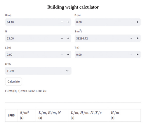
To make the weight prediction model proposed in this paper more user-friendly, an interactive online web page (https://building-weight.streamlit.app) is built and deployed using Streamlit, an open-source Python package, as shown in Figure 8. Users can enter the structural parameters of a building in the interface, and the web page will automatically judge the applicable model according to the input parameters and complete the calculation. Moreover, the online model is updated in real time. After new data is added, the model can be replaced and updated.

7. Conclusion

Aiming at the problem of rapid prediction of RC building’s weight in existing building evaluation and disaster resistance analysis of urban buildings, this paper collected the design data of 732 real engineering cases, presented the regression predictive models of building weight of four structural systems, namely RC F-CW, F-SW, SW, and F, and then tested the applicability and accuracy of these models. Finally, based on the empirical models proposed, an online webpage is developed, which can realize the function of inputting relevant parameters to predict RC building’s weight. The main conclusions are as follows:

1.
The statistical analysis shows that the weight per unit area coefficients recommended in the existing empirical models are small and underestimates the weight of the buildings in China.
2.
Through regression analysis, a series of empirical formulas of building weight are established and validated. It is recommended to first choose the predictive model of the floor area. When the information of the floor area is missing, the predictive model using the structural height or the model using multiple combined parameters can be referred to, and the average value is taken as the final result.
3.
The proposed prediction formulas are deployed on the online web page for users’ convenience. It is important to emphasize that these models are grounded in Chinese building weight data. Variations in the level of building industrialization, construction techniques, commonly used materials, and live load levels across different regions and time periods may introduce uncertainties and affect the accuracy of weight predictions. Regions with higher levels of industrialization tend to adopt prefabricated components or advanced lightweight materials, which can reduce the structural self-weight per unit area. Therefore, in practical applications, it is recommended to use the prediction formulas in conjunction with knowledge of the building’s construction techniques and materials, and to refer to the 95% prediction interval to reasonably estimate the building weight.

There are also several limitations to this study. Firstly, database for developing the prediction models consists only records of buildings designed against Chinese design code since 2010. Thus, the proposed weight prediction models should be used with cautions for RC buildings in other countries. Further studies are necessary to include building records outside China to determine whether the proposed models are also applicable in other countries. Secondly, current model requires manual determination of the type of structure. Although four main types have been considered, it still cannot be applied to all RC structures. Therefore, establishing a single, data-driven predictive model is worth further research.

Conflicts of Interest

The authors declare no conflicts of interest.

Funding

The research was funded by the National Key Research and Development Program of China (Grant No. 2023YFC3805800).

Acknowledgments

The authors appreciate the financial support provided by the National Key Research and Development Program of China (Grant No. 2023YFC3805800).

Open Research

Data Availability Statement

The data that support the findings of this study are available from the corresponding author upon reasonable request.

References

1 Hache E., Simoën M., Seck G. S., Bonnet C., Jabberi A., and Carcanague S., The Impact of Future Power Generation on Cement Demand: An International and Regional Assessment Based on Climate Scenarios, International Economics. (2020) 163, 114–133, https://doi.org/10.1016/j.inteco.2020.05.002.
10.1016/j.inteco.2020.05.002
Google Scholar
2 Huaman J., Anderson F., Mallqui J., Inga A., Zuñiga J. G. B., and Porras F., Self-Built Houses in a Peruvian Andean City: Seismic Vulnerability and Seismic Behavior, Civil Engineering and Architecture. (2023) 11, no. 6, 3488–3504, https://doi.org/10.13189/cea.2023.110619.
10.13189/cea.2023.110619
Google Scholar
3 Cai K., Huang M. F., Wang C. H., Yang C., Ni Y. Q., and Li B. B., A Combined Approach to Estimate Modal Parameters for Updating the Finite Element Model of a High-Rise Building, Structural Control and Health Monitoring. (2024) 2024, no. 1, https://doi.org/10.1155/stc/3650202.
10.1155/stc/3650202
Web of Science® Google Scholar
4 Rezaiee-Pajand M., Entezami A., and Sarmadi H., A Sensitivity-Based Finite Element Model Updating Based on Unconstrained Optimization Problem and Regularized Solution Methods, Structural Control and Health Monitoring. (2020) 27, no. 5, 1–29, https://doi.org/10.1002/stc.2481.
10.1002/stc.2481
Web of Science® Google Scholar
5 Sobhaninejad G., Hori M., and Kabeyasawa T., Enhancing Integrated Earthquake Simulation With High Performance Computing, Advances in Engineering Software. (2011) 42, no. 5, 286–292, https://doi.org/10.1016/j.advengsoft.2010.10.009, 2-s2.0-79956364022.
10.1016/j.advengsoft.2010.10.009
Web of Science® Google Scholar
6 Lu X. Z., Xu Z., Xiong C., and Zeng X., High Performance Computing for Regional Building Seismic Damage Simulation, Procedia Engineering. (2017) 198, 836–844, https://doi.org/10.1016/j.proeng.2017.07.134, 2-s2.0-85029889003.
10.1016/j.proeng.2017.07.134
Google Scholar
7 Hori M., Ichimura T., Wijerathne L. et al., Application of High Performance Computing to Earthquake Hazard and Disaster Estimation in Urban Area, Frontiers in Built Environment. (2018) 4, https://doi.org/10.3389/fbuil.2018.00001, 2-s2.0-85063262250.
10.3389/fbuil.2018.00001
PubMed Google Scholar
8 Xiang M. J., Chen J., Shen J. X., and Wang Z. T., Regional-Scale Stochastic Nonlinear Seismic Time History Analysis of RC Frame Structures, Bulletin of Earthquake Engineering. (2022) 20, no. 15, 8123–8149, https://doi.org/10.1007/s10518-022-01473-1.
10.1007/s10518-022-01473-1
Web of Science® Google Scholar
9 Zeng L. Y., Zhang N., Dou Y., and Zeng H. L., Quantitative Analysis of GIS-based Building Evaluation System in the Renewal of Traditional Industrial Cities, Industrial Construction. (2022) 52, 48–53+162, https://doi.org/10.26914/c.cnkihy.2022.015711.
10.26914/c.cnkihy.2022.015711
Google Scholar
10 Guo J., Miatto A., Shi F., and Tanikawa H., Spatially Explicit Material Stock Analysis of Buildings in Eastern China Metropoles, Resources, Conservation and Recycling. (2019) 146, no. 0, 45–54, https://doi.org/10.1016/j.resconrec.2019.03.031, 2-s2.0-85063649551.
10.1016/j.resconrec.2019.03.031
Web of Science® Google Scholar
11 Ao Z., Hu X. M., Tao S. L. et al., A National-Scale Assessment of Land Subsidence in China’s Major Cities, Science. (2024) 384, no. 6693, 301–306, https://doi.org/10.1126/science.adl4366.
10.1126/science.adl4366
CAS PubMed Web of Science® Google Scholar
12 GB50011-2010, Code for Seismic Design of Buildings (2016 edition), 2016, China Ministry of Construction, China Architecture and Building Press.
Google Scholar
13 JGJ3-2010, Technical Specification for Concrete Structures of Tall Buildings, 2010, China Ministry of Construction, China Architecture and Building Press.
Google Scholar
14 National Technical Measures for Civil Building Engineering Design: 2009 Edition. Structure. Structure System, 2009, China Planning Press.
Google Scholar
15 Aghayere A. O. and Vigil J., Structural Wood Design: A practice-oriented Approach Using the ASD Method, 2007, Wiley.
10.1002/9780470259795
Google Scholar
16 Wang Z. X. and Tsavdaridis K. D., Optimality Criteria-Based Minimum-Weight Design Method for Modular Building Systems Subjected to Generalised Stiffness Constraints: A Comparative Study, Engineering Structures. (2022) 251, https://doi.org/10.1016/j.engstruct.2021.113472.
10.1016/j.engstruct.2021.113472
Web of Science® Google Scholar
17 Jefferson T. Q. and Tatiana S. Q., Dataset of Specific Total Embodied Energy and Specific Total Weight of 40 Buildings From the Last Four Decades in the Andean Region of Ecuador, Data. (2023) 8, no. 5, 1–17, https://doi.org/10.3390/data8050077.
10.3390/data8050077
Google Scholar
18 Parsons T., The Weight of Cities: Urbanization Effects on Earth’s Subsurface, AGU Advances. (2021) 2, no. 1, https://doi.org/10.1029/2020AV000277.
10.1029/2020AV000277
Web of Science® Google Scholar
19 Reshef D. N., Reshef Y. A., Finucane H. K. et al., Detecting Novel Associations in Large Data Sets, Science. (2011) 334, no. 6062, 1518–1524, https://doi.org/10.1126/science.1205438, 2-s2.0-83755163018.
10.1126/science.1205438
CAS PubMed Web of Science® Google Scholar
20 Reshef D. N., Reshef Y. A., Mitzenmacher M. M., and Sabeti P. C., Equitability Analysis of the Maximal Information Coefficient, With Comparisons, Statistics. (2013) .
Google Scholar
21 Theodorsson-Norheim E., Kruskal-Wallis Test: BASIC Computer Program to Perform Nonparametric One-Way Analysis of Variance and Multiple Comparisons on Ranks of Several Independent Samples, Computer Methods and Programs in Biomedicine. (1986) 23, no. 1, 57–62, https://doi.org/10.1016/0169-2607(86)90081-7, 2-s2.0-0022558954.
10.1016/0169-2607(86)90081-7
CAS PubMed Web of Science® Google Scholar
22 Guo S., Zhong S., and Zhang A., Privacy-Preserving Kruskal–Wallis Test, Computer Methods and Programs in Biomedicine. (2013) 112, no. 1, 135–145, https://doi.org/10.1016/j.cmpb.2013.05.023, 2-s2.0-84883746010.
10.1016/j.cmpb.2013.05.023
PubMed Web of Science® Google Scholar
23 Wang Z. T., Chen J., and Shen J. X., Multi-Factor and multi-level Predictive Models of Building Natural Period, Engineering Structures. (2021) 242, https://doi.org/10.1016/j.engstruct.2021.112622.
10.1016/j.engstruct.2021.112622
Web of Science® Google Scholar
24 Wang X. and Chu T. J., Non-Parametric Statistics, 2014, 2nd edition, Tsinghua University Press.
Google Scholar
25 He Y. H., Liu Z., Fu J. Y., Hui Y., and He Y. C., Prediction Models for Modal Parameters of high-rise Buildings Based on the Latest Statistics of Field Measurements, Journal of Building Engineering. (2024) 98, https://doi.org/10.1016/j.jobe.2024.111288.
10.1016/j.jobe.2024.111288
Web of Science® Google Scholar
26 Qian J. R., Zhao Z. Z., and Ye L. P., Structural Design of Tall Buildings, 2012, 2nd edition, China Architecture and Building Press.
Google Scholar
27 GB50009-2012. Load Code for the Design of Building Structures, 2012, China Ministry of Construction, China Architecture and Building Press.
Google Scholar
28 Li A. Q., Yang C., Xie L. L., Liu L. D., and Zeng D. M., Research on the Rational Yield Ratio of Isolation System and Its Application to the Design of Seismically Isolated Reinforced Concrete Frame-Core Tube Tall Buildings, Applied Sciences. (2017) 7, no. 11, https://doi.org/10.3390/app7111191, 2-s2.0-85034627655.
10.3390/app7111191
Google Scholar
29 Yang F. Q., Feng F., and Wei J. J., Analysis and Design of Super high-rise Structure of Shangqiu Financial Center, Building Structure. (2023) 53, no. S1, 69–74, https://doi.org/10.19701/j.jzjg.23S1088.
10.19701/j.jzjg.23S1088
Google Scholar
30 Zhang J. H., Wang X. A., and Meng F. H., Design of Super Large-Span Connected Structure of a Middle School Administrative Building, Low Temperature Architecture Technology. (2023) 45, no. 2, 90–94+98, https://doi.org/10.13905/j.cnki.dwjz.2023.2.019.
10.13905/j.cnki.dwjz.2023.2.019
Google Scholar
31 Engineering Research Institute of Appraisal and Strengthening of Shandong Jianzhu University Co Ltd, The World’s First Irregular Fan-Shaped Vehicle Arrangement, the Largest Single Building Area for Trailer Relocation in China (4658 m²), and the Heaviest Single Building Weight for Trailer Relocation in China (7500 Tons), 2023, https://mp.weixin.qq.com/s/V3H4dRIgc5Ei8ALmz7KGMg.
Google Scholar

All articles

Predictive Model for Estimating the Weight of Existing RC Buildings Using Easily Accessible Structural Parameters

Abstract

1. Introduction