One-Dimensional Deep Convolutional Neural Network-Based Intelligent Fault Diagnosis Method for Bearings Under Unbalanced Health and High-Class Health States
Abstract
Modern industrial systems depend heavily on rotating machines, especially rolling element bearings (REBs), to facilitate operations. These components are prone to failure under harsh and variable operating conditions, leading to downtime and financial losses, which emphasizes the need for accurate REB fault diagnosis. Recently, interest has surged in using deep learning, particularly convolutional neural networks (CNNs), for bearing fault diagnosis. However, training CNN models requires extensive data and balanced bearing health states, which existing methods often assume. In addition, while practical scenarios encompass a diverse range of bearing fault conditions, current methods often focus on a limited range of scenarios. Hence, this paper proposes an enhanced method utilizing a one-dimensional deep CNN to ensure reliable operation, with its effectiveness evaluated on Case Western Reserve University (CWRU) rolling bearing datasets. The experimental results showed that the diagnostic accuracy reached 100% under 0∼3 hp working loads for 10 unbalanced health classes. Moreover, it attained 100% accuracy for high-class health states with 20, 30, and 40 classes, and when extended to 64 health classes, it reached a peak accuracy of 99.96%. Thus, the method achieved improved classification ability and stability by employing a straightforward model architecture, along with the integration of batch normalization and dropout operations. Comparative analysis with existing diagnostic methods further underscores the model superiority, particularly in scenarios involving unbalanced and high-class health states, thus emphasizing its effectiveness and robustness. These findings significantly advance the field of intelligent bearing fault diagnosis.
1. Introduction
Rotating machinery plays a crucial role in various industrial fields, such as aerospace, automotive, aviation, and manufacturing, accounting for over 90% of modern industrial machines [1]. Rolling element bearings (REBs) are vital components in these machines, primarily used to reduce friction, absorb stress, and facilitate motion during operation [2, 3]. However, the health status of REBs greatly affects machines, with vulnerabilities to diverse failures due to changing operating conditions such as extreme temperatures, overloading, high moisture levels, and high-speed operations [4]. The existing studies show that 45%–55% of machine breakdowns result from REB faults, with common fault types including ball faults, outer race faults, inner race faults, and cage faults [5]. Kateris et al. [6] found that around 90% of REB faults are caused by cracks in the inner and outer races, with the remaining 10% due to cracks in the balls or cages. The occurrence of any such failures can halt machinery operations, resulting in substantial financial losses, high maintenance costs, and overall safety concerns. Hence, bearing fault diagnosis is crucial in industrial machinery to prevent operational interruptions, minimize financial losses, reduce maintenance expenses, and enhance personal safety.
Fault diagnosis involves identifying either the specific fault that occurred or the reasons behind an abnormal or out-of-control status. It includes detecting, isolating, and identifying the components (or subsystems and systems) that have ceased to operate [7]. Fault detection identifies abnormal conditions, followed by fault isolation to pinpoint failing components. Finally, fault identification assesses the type and severity of the fault.
Over the years, numerous fault diagnosis methods have emerged for bearings. These methods are broadly categorized into knowledge-based, model-based, and data-driven-based methods [8, 9]. Knowledge-based approaches use expert systems and diagnostic databases, relying on domain expertise but limited by knowledge accuracy. In contrast, model-based methods employ mathematical models, signal processing, and parameter estimation but require precise system dynamics and struggle with complex faults [10]. Recently, data-driven fault diagnosis methods have become increasingly popular due to rapid advancements in data mining techniques [11]. These methods utilize machine learning (ML) and data analysis techniques to identify faults effectively without heavy reliance on prior knowledge. By leveraging large datasets, data-driven fault diagnosis methods can handle complex fault patterns and extract relevant features from raw sensor data, such as acoustic emission, vibration, and current [12, 13]. Among data-driven methods, artificial intelligence (AI)-based fault diagnosis techniques utilizing vibration signals for bearings have garnered significant attention and recognition recently. These methods are valued for their reliability, robustness, and adaptive capabilities, emerging as powerful tools for processing vast datasets and diagnosing faults in mechanical equipment [14]. With the rapid advancements in the field of AI, literature suggests that AI-based fault diagnosis in rotating machinery can be categorized into two main groups: traditional ML and deep learning (DL) approaches.
Traditionally, ML-based methods have been extensively employed for bearing fault diagnosis in rotating machinery. ML theories have served as the foundation of intelligent fault diagnosis (IFD) from its inception through the 2010s [15]. These methods encompass the utilization of various algorithms, such as support vector machines [16], artificial neural networks (ANN) [17], and k-nearest neighbors [18], to extract features and classify faults based on vibration signals. While these approaches have shown promising results, manual feature engineering is often required, and capturing complex patterns in the data can be challenging [19]. In response to the limitations of traditional ML approaches, modern IFD technology has evolved, integrating novel theories and AI techniques. This evolution has given rise to DL-based fault diagnosis methods, which have proven highly effective and gained significant attention. DL, introduced by Hinton and Salakhutdinov [20], has become prominent in machine fault diagnosis since around 2015, enabling automatic feature extraction from raw input data and enhancing diagnosis accuracy. Notable DL methods, such as deep belief networks [21], stacked autoencoders [22], convolutional neural networks (CNNs) [23], recurrent neural networks [24], and generative adversarial networks [25], have demonstrated remarkable capabilities in learning hierarchical representations from raw vibration data.
In particular, CNNs have proven to be highly effective in analyzing vibration signals, demonstrating their ability to capture localized patterns and features in time-series data. Compared with other neural networks, CNN-based bearing fault diagnosis methods have achieved remarkable success, offering advantages such as flexible input formats, various improvement techniques, high classification accuracy, and the ability to capture spatial properties of fault data. With features such as sparse local connections, weight sharing, and down-sampling, CNNs excel in bearing fault diagnosis and are widely applied [26]. In addition, these features reduce computational complexity and mitigate overfitting, thereby enhancing both pattern recognition accuracy and efficiency. Various CNN architectures have been developed for bearing fault diagnosis, with one-dimensional CNNs (1D-CNNs) and two-dimensional CNNs (2D-CNNs) being the most commonly used.
Traditional 2D-CNNs convert 1D vibration signals into 2D images, using spectrograms or time-frequency representations to capture spatial patterns and frequency correlations for feature extraction. In line with this motivation, Janssens et al. [27] demonstrated the efficacy of this approach by transforming original time domain data into frequency domain representations as input for a 2D-CNN model for bearing fault diagnosis. To address limitations of shallow 2D-CNNs, Wang et al. [28] proposed a bearing diagnosis model utilizing a multiheaded attention mechanism. However, 2D-CNNs face challenges in preserving temporal features from vibration signals, limiting effectiveness in bearing fault diagnosis. In addition, increased processing time, higher computational resource consumption, and potential data loss occur during the transformation of raw vibration signals into image.
To overcome these limitations, researchers have developed 1D-CNNs to process raw time-series data directly, capturing temporal dependencies and variations more effectively. The 1D-CNNs provide potential enhancements to bearing fault diagnosis models by learning relevant features without preprocessing or data transformation. For example, She and Jia [29] introduced a fault diagnosis method for rolling bearings using multichannel signal data with a multichannel 1D-CNN. In addition, Wang et al. [30] improved interpretability in wheelset bearing diagnosis by integrating channel attention mechanisms into 1D-CNN. Furthermore, Ince et al. [31] combined an improved 1D-CNN with motor current signals for real-time monitoring of bearing faults.
Despite the demonstrated success of 1D-CNNs in diagnosing bearing faults, several challenges remain unaddressed. One major issue is the need for large, balanced datasets to effectively train 1D-CNN models. In real-world scenarios, however, there is often a lack of sufficient faulty data, leading to imbalanced datasets and reduced diagnostic accuracy. As a result, existing 1D-CNN-based methods typically assume balanced training data across all bearing health states. Another significant challenge is the limited consideration of fault scenarios in current research. Practical bearings encounter a wider range of fault conditions due to varying speeds and loads. This discrepancy between the narrow fault scenarios studied and the diverse conditions found in real-world applications hinders accurate fault classification. Moreover, existing 1D-CNN-based models often struggle to classify fault conditions across various categorized high-class health states, typically performing well only in single-categorized health states. However, in practice, machines can fail unexpectedly due to fluctuating conditions, making accurate fault classification even more challenging. Therefore, further research into 1D-CNN-based methods is essential to enhance performance and ensure robustness by addressing these challenges in bearing fault diagnosis.
To address this gap, the primary goal of this paper was to propose an enhanced bearing fault diagnosis method using a one-dimensional deep CNN (1D-DCNN). The proposed method is designed to handle unbalanced and high-class health states under varying load conditions, ensuring the safe and reliable operation of rotating machines. Initially, the approach utilized a segmentation process to convert 1D vibration signals into segmented samples, leveraging segmentation for time-domain feature extraction and employing 1D-DCNN for health classification. This method ensured no information loss during segmentation, reduced resource consumption, and minimized processing time. In addition, model performance was optimized by reducing convolutional layers, decreasing kernel size, integrating batch normalization (BN), and applying dropout operations. To further ensure the robustness of the proposed method, a comprehensive ablation study was conducted to assess the impact of key network parameters and training hyperparameters on model performance. The effectiveness of the proposed method was evaluated using the Case Western Reserve University (CWRU) motor rolling bearing dataset, categorized in two ways. First, it was assessed under four distinct loading conditions: 0, 1, 2, and 3 hp, each consisting of 10 unbalanced bearing health states. Second, it was evaluated across four different categorized unbalanced high-class health states: 20, 30, 40, and 64 health classes, under varying loading conditions (0∼3 hp). The experimental findings are compared against state-of-the-art CNN-based techniques and emphasize the proposed method superior performance.
The remaining sections of the paper are organized as follows: Section 2 describes the theoretical background of CNNs and advancements in bearing fault diagnosis. Section 3 elaborates on the research methodology, including the model architecture, fault diagnosis procedures, and evaluation techniques. Section 4 presents experimental validations, covering data preprocessing, network parameter selection, and diagnostic results, along with a comparative analysis against state-of-the-art methods. Finally, the last section provides the conclusions and summarizes the study.
2. Theoretical Background of CNNs
Due to its fast computation, high accuracy, and robust performance, AI has gained increasing attention from both academia and industry, reducing reliance on expert knowledge. Various AI techniques, including DL, have been effectively applied across multiple domains, such as healthcare [32] and face recognition [33]. Beyond these applications, AI also plays a crucial role in state prediction and equipment safety [34], predictive maintenance, enabling accurate equipment failure forecasts, and remaining useful life prediction [35], as well as intelligent machinery fault diagnosis (IMFD) [36]. In IMFD, among AI methods, CNNs have emerged as a powerful and highly effective tool for diagnosing machine faults, especially for detecting bearing faults. Inspired by neural structures in the animal brain, CNNs were first introduced in 1994 for image pattern recognition [37]. The concept of receptive fields, common in ANN, plays a crucial role in CNN, simulating biological computations. CNN stands out from other deep neural networks due to its sparse connections and weight-sharing mechanisms [38]. Sparse connections establish limited spatial links between adjacent layers using a topological structure, while weight sharing involves applying a set of filtering parameters uniformly across the entire convolutional layer. These characteristics enable CNN to significantly reduce the number of training parameters and prevent overfitting, especially with high-dimensional data inputs.
2.1. Principle and Architecture of CNN
A CNN is a multistage neural network structured with multiple filtering stages and a final classification stage. Figure 1 illustrates the standard CNN architecture, beginning with an input, followed by a feature extraction block that includes convolution, activation functions (AFs), and pooling layers. This block is followed by fully connected layers, leading into the final classification stage [39, 40].

Convolution layers extract features by applying fixed-size filter kernels to local input regions, generating feature maps through activation units [38]. As illustrated in Figure 2, this involves concepts such as tensors, kernels, and feature maps, where a dot product between the kernel and input tensor is computed to generate feature map values. This linear operation is fundamental in image processing, where matrices are convolved with smaller kernel matrices.
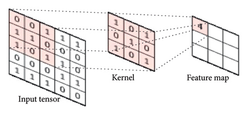
After convolution, AF nonlinearly transform output values, improving the network’s ability to represent input data and distinguish learned features [5]. The Rectified Linear Unit (ReLU) is popular in convolution layers for its effective half-rectified nature that accelerates convergence.
Next, the pooling layer serves as a downsampling operator, consolidating semantically similar features and thereby reducing the network’s dimensions and parameters. Two frequently used pooling methods are average pooling, which calculates the mean value of each patch on the activation map, and maxpooling, which identifies the maximum value within each patch of the feature map [42]. Figure 3 illustrates the maxpooling operation, where the largest element within the filter area in the input matrix is selected.
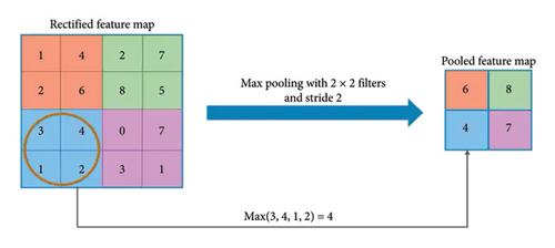
The subsequent step involves transforming the output of the convolutional block into a one-dimensional array for input into the next layer, known as the fully connected layer, as depicted in Figure 4. The final layer is the classification layer, which categorizes objects into their respective classes [44]. For multiclass classification tasks, the Softmax AF is typically used to ensure each class probability ranges between 0 and 1, with the sum of all probabilities equaling 1. Hence, the highest output value determines the final classification [5].
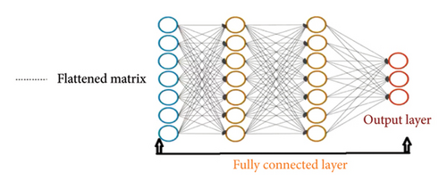
In addition, to expedite training and improve convergence in CNN networks, the BN layer, as proposed by [45], is incorporated. It mitigates internal covariance shifts, thereby enhancing both training efficiency and generalization capabilities. Moreover, dropout is a regularization technique used in neural networks to prevent overfitting. During training, it randomly deactivates a portion of neuron units and their connections within the network, effectively creating an ensemble of multiple networks. This approach helps the network generalize better to new data, reducing the risk of overfitting [46].
2.2. CNN-Based Bearing Fault Diagnosis Method
CNNs and their various variants are extensively used in machine fault diagnosis, particularly for detecting bearing faults. Methods in this area have advanced significantly, enabling the effective capture of localized patterns and features in time-series data, especially vibration signals [47]. Common models for bearing fault diagnosis include 1D-CNNs and 2D-CNNs, which are widely applied in time-frequency analysis.
The 2D-CNN, derived from LeNet-5, is designed for image processing, generating 2D matrix outputs from inherently 3D input and output. Its strength lies in extracting spatial features via kernels, making it highly effective for tasks such as image classification and spatial data analysis, including edge detection and color distribution. In bearing fault diagnosis, researchers have adapted 2D-CNNs by converting 1D vibration signals into 2D images for more efficient feature extraction. Given the challenges in obtaining accurate fault data from rotating machinery, 2D-CNN-based data augmentation, which transforms raw data, has proven to be an effective solution [27]. For instance, Wang et al. [28] developed a 2D-CNN model with a multiheaded attention mechanism to improve bearing fault diagnosis. Some researchers optimized 2D-CNNs with attention mechanisms, reducing parameters and boosting accuracy. For example, Wang et al. [48] introduced a squeeze-and-excitation-enabled 2D-CNN to further minimize parameters for intelligent bearing fault diagnosis. In addition, researchers have incorporated multisensor data for both data-level and feature-level fusion to improve model performance. Guo et al. [49] used multilinear subspace learning to integrate multichannel datasets into 2D-CNN, while Liu et al. [50] introduced a feature fusion technique for better rotating equipment fault detection.
On the other hand, in the domain of CNNs, a 1D-CNN uses a filter that moves along a single direction, typically the temporal axis, producing a 1D array output from 2D input. The 1D-CNNs are commonly used for accelerometer, time-series, and sensor data, making them popular for text and audio analysis. In addition, 1D-CNNs are extensively employed in intelligent machine fault diagnosis, particularly for bearing faults, utilizing raw vibration data without signal preprocessing [51]. Multiple filters enable distinct feature extraction from signal series. For instance, Zhao et al. [52] utilized normalized single-scale 1D data for diagnosing rolling bearing faults. Likewise, Ince et al. [31] combined an improved 1D-CNN with motor current signal input for real-time monitoring of motor bearing faults diagnosis. Moreover, She and Jia [29] proposed a fault diagnosis approach for rolling element bearings that involves feeding multichannel signal data into a multichannel 1D-CNN.
Overall, using 2D-CNNs, data transformation, or signal processing can increase complexity, potentially reducing efficiency and intelligence. However, converting 1D raw data into 2D images aids in data augmentation, especially for bearing faults. In contrast, 1D-CNN models, which process raw 1D vibrational data, can establish a comprehensive diagnostic framework without domain expertise. These methods are effective in bearing fault diagnosis by learning features directly from raw time-series data, capturing temporal dependencies, and extracting distinct features through multiple filters. 1D-CNNs offer advantages over 2D-CNNs, including better temporal information capture, reduced processing time, lower resource use, and no information loss.
3. Proposed Method
In these sections, the proposed method for diagnosing unbalanced and high-class bearing health states under varying loading conditions using an enhanced 1D-DCNN is presented. This study introduces a technique called 1D segmented vibration data with an enhanced deep 1D-CNN model. Detailed descriptions of the proposed methods, including the 1D-DCNN model architecture, fault diagnosis process, and evaluation techniques, are provided.
3.1. Model Network Structure Development
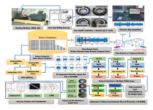
The structure and parameter settings for the enhanced 1D-DCNN model in this study were determined through multiple experiments and random search methods. In addition, an ablation study was conducted to emphasize the critical role of selecting key network parameters and training hyperparameters in enhancing model performance. As a result, the overall structure of the proposed 1D-DCNN model was developed using the Keras Sequential API, following the standard CNN framework. This architecture consists of convolutional layers for feature extraction and fully connected layers for classification. Notable modifications include the integration of BN and dropout after each convolutional layer, along with dropout in the fully connected layer.
Consequently, the proposed architecture comprises three convolutional layers followed by pooling layers and three fully connected layers. Each convolutional layer employs the ReLU AF, along with BN and dropout layers to enhance performance and prevent overfitting. In addition, a dropout layer is incorporated into the fully connected layer to further mitigate overfitting. The final dense (output) layer utilizes the Softmax AF for multiclass classification. Using multilayer small convolutional kernels deepens the network, enabling robust representations of 1D segmented vibration signals and improving overall performance. The complete architecture of the proposed 1D-DCNN model, including all described layers and operations, is depicted in Figure 5.
3.2. Bearing Fault Diagnosis Process
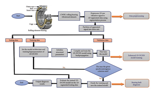
The proposed method for diagnosing bearing faults under unbalanced and high-class health states across varying loading conditions relies on a 1D segmented vibrational signal and a 1D-DCNN model. The diagnostic process comprises three main steps.
First, the 1D raw vibration data are preprocessed and transformed into 1D segmented vibration data, which is then divided into training, validation, and testing sets. Next, the network parameters and training hyperparameters of the 1D-DCNN model are configured, and the model parameters are initialized. During training, the model is fed with segmented vibration data from the training set. Using backpropagation and gradient descent, the model parameters are adjusted to minimize the loss function. This iterative process continues until convergence or a predefined stopping criterion is met. In addition, the model is fine-tuned using validation data during training. Hyperparameters and model performance are optimized based on feedback from the validation set. Lastly, once the model performance is satisfactory, it is tested using the testing data. The segmented vibration data from the testing set are input into the trained model, generating fault diagnosis predictions. These predictions indicate the presence and nature of faults in the bearing system. Figure 6 visually represents the sequential steps of the proposed method, guiding the implementation and understanding of the fault diagnosis process.
3.3. Model Evaluation Techniques
Following the training phase of the 1D-DCNN model, its performance is evaluated by estimating generalization accuracy using unseen test data. For classification and detection tasks, common evaluation metrics include accuracy, precision, recall, and F1-score. The proposed work incorporates a range of evaluation techniques to assess the effectiveness and performance of the model, including classification accuracy metrics, confusion matrix, classification report results (precision, recall, and F1-score) and dimensional reduction using t-Distributed Stochastic Neighbor Embedding (t-SNE). These diverse evaluation methods provide valuable insights into the model’s performance and generalization capabilities.
4. Experimental Validation
During the experimental phase of diagnosing bearing faults for classification, an enhanced 1D-DCNN model is utilized to classify health states from two perspectives. First, it classifies bearing health states under four different loading conditions: 0, 1, 2, and 3 hp, each containing 10 unbalanced health states. Subsequently, it is evaluated under four different cases, as unbalanced high-class health states: 20, 30, 40, and 64 health classes, across varying loading conditions (0∼3 hp). The experimental validations encompass descriptions of bearing datasets, data preparation, preprocessing, and partition. In addition, they include the selection of network parameters and training hyperparameters, diagnosis results, and comparisons with existing methods.
4.1. Datasets Description
In this study, the effectiveness of the proposed enhanced 1D-DCNN model was assessed using the public vibration dataset obtained from the CWRU motor bearing datasets [53]. It has been widely used in machine fault diagnosis research, particularly for diagnosing bearing faults. The dataset originates from The CWRU test rig, depicted in Figure 7, was used for collecting the vibration data.
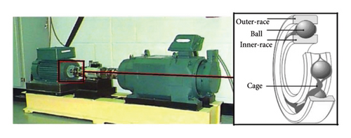
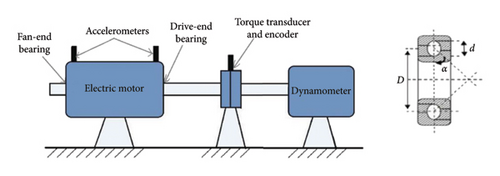
As depicted in Figure 7, the test stand includes key components: a 2-horsepower motor on the left, a torque transducer/encoder in the center, and a dynamometer on the right side. Accelerometers were strategically positioned at the 12 o’clock position on both the drive end and fan end of the motor housing, and faults were simulated using electrodischarge machining. Based on the provided description, the vibration datasets utilized in this study were obtained from the drive end of the test rig, featuring a 6205-2RS JEM deep groove ball bearing manufactured by SKF. The datasets were sampled at 12 kHz and encompassed four load conditions with varying rotational speeds: 0 hp/1797 rpm, 1 hp/1772 rpm, 2 hp/1750 rpm, and 3 hp/1730 rpm. In addition, bearing faults were intentionally introduced in the inner race, ball, and outer race, along with a normal condition, with fault severity varied by employing different fault diameters: 0.007, 0.014, 0.021, and 0.028 inches. Overall, the dataset comprises a total of 60 health classes for fault conditions and 4 classes for normal conditions, all utilized to evaluate the proposed enhanced 1D-DCNN model.
4.2. Data Preparation
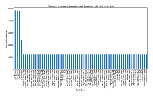
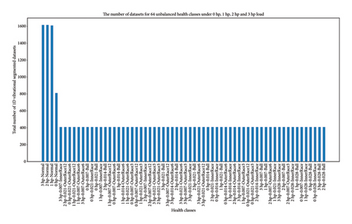
In this study, Python, along with the SciPy library, was utilized to extract raw 1D vibration data from MATLAB format. The extracted data was then processed and consolidated into a single CSV file using Pandas, ensuring efficient organization of drive-end acceleration data and labels for seamless manipulation. As a result, the data preparation process for the proposed work was structured in two main ways. First, the datasets were categorized by bearing health states under four loading conditions (0∼3 hp), where each load level (0, 1, 2, and 3 hp) contains 10 health classes, including one normal and nine fault conditions. Next, the dataset was categorized into four unbalanced high-class health states: 20, 30, 40, and 64 health classes under varying load conditions. Specifically, the 20-health-class scenario includes 0 and 1 hp loads with 2 normal and 18 fault conditions; the 30-health-class case adds 2 hp loads, totaling 3 normal and 27 fault conditions; the 40-health-class scenario covers 0∼3 hp loads with 4 normal and 36 fault conditions, while the 64-health-class case expands to all classes, comprising 4 normal and 60 fault conditions under 0∼3 hp loads. Based on the preceding sections, Figure 8 illustrates the data preparation methods for all 64 health states, with health class labels on the x-axis and the total number of dataset samples on the y-axis.
4.3. Network Parameters and Training Hyperparameter Selection for the 1D-DCNN Model
4.3.1. Ablation Study on Key Network Parameters and Training Hyperparameters
To ensure the robustness of the proposed method, a comprehensive ablation study was conducted to evaluate the impact of key network parameters and training hyperparameters on model performance. The parameters examined included input shape, number of Conv Layers, BN, dropout rates, learning rate, batch size, and the number of epochs. These parameters were identified through a series of experiments guided by random search methods. The findings from this ablation study, summarized in Table 1, demonstrate that selecting appropriate network parameters and training hyperparameters significantly influences the model’s generalization ability and its accuracy in diagnosing bearing faults.
| No | Parameter | Tested values | Optimal value | Observation |
|---|---|---|---|---|
| 1 | Input shape | 784 × 1, 1024 × 1, 2048 × 1, segments | 784 × 1 | Effectively preserves fault signal features (1D segmented vibrational signal) while minimizing computational overhead |
| 2 | Number of conv layers | 2, 3, 4 | 3 | Deeper models yield minimal improvement; fewer layers result in underfitting |
| 3 | BN | Yes/No | Yes | Enhances model stability, accelerates convergence, and improves generalization |
| 5 | Dropout (conv layers) | 0.3, 0.5, 0.7 | 0.5 | Strikes optimal balance between regularization and feature preservation |
| 6 | Dropout (dense layer) | 0.1, 0.2, 0.3 | 0.2 | Reduces overfitting while retaining essential features for accurate classification |
| 7 | Learning rate | 0.01, 0.001, 0.0001 | 0.001 | Stabilizes training, ensures smoother convergence, and improves accuracy |
| 8 | Batch size | 50, 100, 200 | 200 | Best trade-off between accuracy and training speed |
| 9 | Number of epochs | 50, 100, 200 | 100 | Training beyond 100 epochs leads to overfitting; fewer epochs result in underfitting |
This ablation study emphasizes the critical role of selecting optimal network parameters and training hyperparameters in enhancing the performance of the 1D-DCNN model. By fine-tuning these values, the proposed method ensures superior accuracy, stability, and generalization, reinforcing its effectiveness for intelligent bearing fault diagnosis. Building on the insights gained from the ablation study, further exploration of optimal parameters for the remaining variables was conducted through experiments guided by random search methods. The optimal selection of all network parameters and training hyperparameters for this study is presented in Table 2, providing a comprehensive overview of the essential elements for constructing and optimizing the 1D-DCNN model. The proposed model architecture is designed to enhance performance and accuracy, particularly under unbalanced and high-class health states across varying load conditions.
| 1D-DCNN model | Parameters | Common selected parameters | No. of layers | Network parameters inside of layers | No specifications |
|---|---|---|---|---|---|
| Keras sequential API | Model network parameters | Input layer | 1 | — | In the input layer, the input shape is defined as 784 × 1 |
| Convolutional layers (1D conv layer) | 3 | Filters | In each layer, there are three filters, with 64, 64, and 32 filters | ||
| Kernel size | Likewise, the three kernel sizes, specifically 100, 100, and 50 | ||||
| Activation functions | In each layer, ReLU is utilized | ||||
| 1D pooling layers | 3 | MaxPooling1D | In each 1D conv layer, a 2 × 2 pool size is used | ||
| Full-connected layers/dense layers | 3 | Neurons | In the first two dense layers, 100 and 50 neurons are employed | ||
| In the last dense layer, it utilizes the total number of fault classes | |||||
| Activation functions | In the first two dense layers, ReLU activation is employed | ||||
| In the last dense layer, Softmax activation is employed | |||||
| Training hyperparameters | Hyperparameters | No. of hyperparameters | No specifications | ||
| BN layer | 3 | To normalize for faster training, each 1D conv layer incorporates | |||
| Dropout layer | 4 | Each conv layer incorporates dropouts with a size of 0.5 and a 0.2 in the second dense layer | |||
| Loss functions | — | Categorical cross-entropy loss is utilized to efficiently manage multiclass classification tasks | |||
| Optimizer | — | The Adam optimizer is utilized with the specified learning rate | |||
| Batch size | — | A batch size of 200 samples per gradient update is employed | |||
| Learning rate and epochs | — | The learning rate of 0.001 is utilized over 100 epochs for iterations over the entire training | |||
4.3.2. Model Initialization and Training Configuration
Once the 1D-DCNN model parameters were initialized, Table 3 presents a detailed summary and provide a comprehensive breakdown of each layer and its corresponding output parameters. Initially, the 1D vibration data were segmented and fed into the 1D-DCNN model, which consisted of three convolutional layers and three pooling layers, yielding 128 feature maps of dimensions 36 × 1. These feature maps were then flattened into a 1152-dimensional vector, serving as input for the fully connected layers. To enhance model performance, dropout regularization was applied during training, while BN was integrated into all three convolutional layers, with scaling and bias parameters initialized randomly. The classifier then comprised two fully connected layers with 100 and 50 neurons, respectively, producing an output size of 10, corresponding to 10 different working conditions. In addition, the model accounted for 20, 30, 40, and 64 unbalanced high-class health states under varying working conditions. The proposed model employed categorical cross-entropy as the loss function, while Softmax was used as the AF in the final layer. The Adam optimizer was selected for training, with a learning rate of 0.001 to update network parameters over 100 epochs. Furthermore, batch size selection significantly impacted both training speed and model accuracy. Through an ablation study, a batch size of 200 was identified as optimal under varying loading conditions.
| Layer (type) | Output shape | Parameter |
|---|---|---|
| conv1d_1 (Conv1D) | (None, 685, 64) | 6464 |
| batch_normalization_1 (BN) | (None, 685, 64) | 256 |
| max_pooling1d_1 (maxpooling 1D) | (None, 342, 64) | 0 |
| dropout_1 (Dropout) | (None, 342, 64) | 0 |
| conv1d_ 2 (Conv1D | (None, 243, 64) | 409,664 |
| max_pooling1d_ 2 (Maxpooling 1D) | (None, 121, 64) | 0 |
| batch_normalization_ 2 (BN) | (None, 121, 64) | 256 |
| dropout_2 (dropout) | (None, 121, 64) | 0 |
| conv1d_3 (Conv1D) | (None, 72, 32) | 102,432 |
| max_pooling1d_ 3 (Maxpooling 1D) | (None, 36, 32) | 0 |
| batch_normalization_3 (BN) | (None, 36, 32) | 128 |
| dropout_3 (Dropout) | (None, 36, 32) | 0 |
| flatten_ (Flatten) | (None, 1152) | 0 |
| dense_1 (Dense) | (None, 100) | 115,300 |
| dropout_ (Dropout) | (None, 100) | 0 |
| dense_2 (Dense) | (None, 50) | 5050 |
| After the second-to-last layer for each categorized class, the following total parameters were obtained: | ||
| dense_3 (dense) | (None, 10) | 510 |
| 10 health classes under four varying loading conditions (0 hp/1 hp/2 hp/3 hp) | Total params: 640,060 | |
| Trainable params: 639,740 | ||
| Non-trainable params: 320 | ||
| dense_3 (dense) | (None, 20) | 1020 |
| 20 health classes under 0 and 1 hp load conditions | Total params: 640,570 (2.44 MB) | |
| Trainable params: 640,250 (2.44 MB) | ||
| Non-trainable params: 320 (1.25 KB) | ||
| Dense_3 (dense) | (None, 30) | 1530 |
| 30 health classes under 0, 1, and 2 hp load conditions | Total params: 641,080 (2.45 MB) | |
| Trainable params: 640,760 (2.44 MB) | ||
| Non-trainable params: 320 (1.25 KB) | ||
| Dense-3 (dense) | (None, 40) | 2040 |
| 40 health classes under 0, 1, 2, and 3 hp load conditions | Total params: 641,590 (2.45 MB) | |
| Trainable params: 641,270 (2.45 MB) | ||
| Nontrainable params: 320 (1.25 KB) | ||
| Dense_3 (dense) | (None, 64) | 3264 |
| 64 health classes under 0, 1, 2, and 3 hp load conditions | Total params: 642,814 (2.45 MB) | |
| Trainable params: 642,494 (2.45 MB) | ||
| Nontrainable params: 320 (1.25 KB) | ||
4.4. Data Preprocessing and Bearing Diagnosis Results
4.4.1. Data Preprocessing Results
In this study, specific data preprocessing techniques were developed to leverage temporal information in 1D raw vibration data, enhancing feature learning and diagnostic accuracy in the 1D-DCNN model. The chosen method involves segmenting time-domain data using predefined window and stride lengths, transforming the 1D raw vibration data into segmented 1D vibration signals, as illustrated in Figure 9.

Here, the window length represents the size of each segment, while the stride denotes the step size between consecutive windows. After extensive experimentation and an ablation study, a window size of 784 and a stride of 300 were identified as the optimal parameters for effectively capturing essential features within each category. These parameters were carefully chosen to enhance pattern extraction from the data, improving the model ability to analyze raw 1D vibration data and enabling efficient training for accurate multiclass bearing fault diagnosis.
Hence, data preprocessing for the proposed work builds upon the data preparation in Section 4.2. First, the organized data under four load conditions (0∼3 hp), each with 10 unbalanced health states, undergoes segmentation. After reshaping, the data dimensions under different loads are as follows: (4452, 784, 1) and (4452, 10) for 0 hp, indicating 4452 samples with 784 data points and 10 health states; similarly, (5251, 784, 1) and (5251, 10) for 1 hp; (5253, 784, 1) and (5253, 10) for 2 hp; and (5263, 784, 1) and (5263, 10) for 3 hp. Figure 10 illustrates the total number of segmented datasets across the 10 unbalanced health states under varying load conditions.
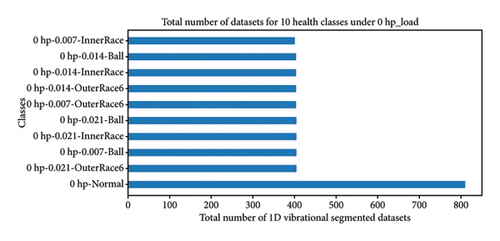
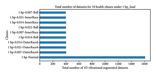
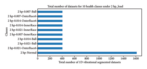
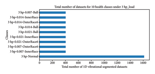
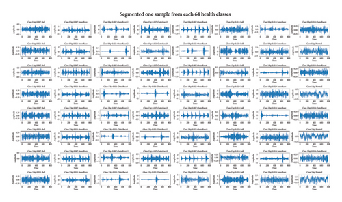
Subsequently, the prepared data undergo preprocessing for four categorized unbalanced high-class health states: 20, 30, 40, and 64 classes across varying load conditions (0∼3 hp). The dataset dimensions are (9703, 784, 1) and (9703, 20) for 20 classes, (14,956, 784, 1) and (14,956, 30) for 30 classes, (20,219, 784, 1) and (20,219, 40) for 40 classes, and (29,909, 784, 1) and (29,909, 64) for 64 classes. Figure 11 shows the segmented datasets for each of the 64 health classes under 0∼3 hp load conditions, while Figure 12 displays a single segmented sample from each of the 64 health classes and provides a clear view of the 1D vibration data in the time domain.
4.4.2. Data Partitioning Results
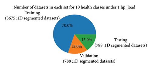
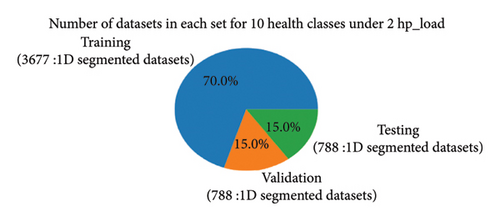
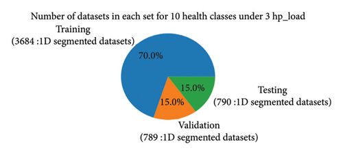
To efficiently train and assess the model, the 1D segmented dataset was divided into three subsets: training, validation, and testing sets. Based on the literature review and experimentation, the data partitioning process involved the following steps. Initially, the data within each class were shuffled for randomness. Then, the data were partitioned with 70% allocated to the training set and 30% to the combined validation and testing set, with 15% for validation and 15% for testing. After data processing, the data splitting process for the proposed method begins with four load conditions (0∼3 hp), as illustrated in Figure 13, which shows the distribution of datasets across health classes in the training, validation, and testing subsets. Next, the data are partitioned for the categorized cases of unbalanced high-class health states: 20, 30, 40, and 64 classes under various load conditions, similarly.

4.4.3. Bearing Diagnosis Results and Analysis
The proposed model was developed and tested on an HP laptop running Windows 10 Enterprise, equipped with an Intel Core i5-6300U CPU (2.40–2.50 GHz), 8GB RAM, 1TB HDD, and 256GB SSD. Python was used for model development and training, utilizing libraries such as NumPy, Pandas, Matplotlib, SciPy, Seaborn, Keras, and TensorFlow. This section presents the bearing fault diagnosis results for unbalanced health and high-class health states using the proposed 1D-DCNN model.
4.4.3.1. Bearing Diagnosis Results Under Four Different Loading Conditions: 0, 1, 2, and 3 hp Loads
The results of bearing fault diagnosis for unbalanced health classes under 0∼3 hp load conditions, each with 10 health classes, are discussed. The diagnosis was performed using the proposed 1D-DCNN model and evaluated based on classification accuracy, confusion matrix, classification report, and t-SNE dimensionality reduction.
4.4.3.1.1. Bearing Diagnosis Results Utilizing Classification Accuracy Metrics. In this scenario, the 1D-DCNN model for bearing fault diagnosis, trained over 100 epochs with a batch size of 200 under 10 health states for four varying load conditions, demonstrated remarkable performance. Accuracy increased progressively, reaching 99% by the 10th epoch for each load condition and eventually achieving 100% on the training dataset by the 40th epoch. In addition, accuracy on the validation data improved steadily, reaching 100% by the 45th epoch under 0∼3 hp loads. These results were highly promising, with accuracy continuously rising throughout the training process. Figure 14 shows the accuracy and loss curves, indicating effective learning and successful loss function minimization, underscoring the model effectiveness and ability to generalize well.
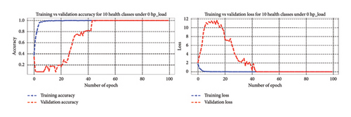
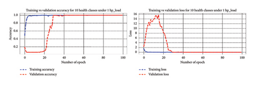
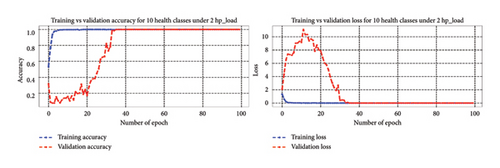
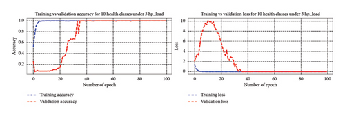
The 1D-DCNN model exhibited strong learning capabilities and achieved high accuracy on both the training and validation sets for unbalanced health states under four varying load conditions. After training and validation, the model’s effectiveness was evaluated using the testing dataset for each load condition. The 1D-DCNN model demonstrated outstanding performance on the test dataset, achieving a remarkably low-test loss of 0.0000 and a test accuracy of 1.0000. These results indicate flawless performance on unseen test data and emphasize its precision and accuracy in bearing fault classification. Overall, the 1D-DCNN model proved to be robust, effective, and reliable in diagnosing bearing faults, consistently achieving high performance across varying load conditions.
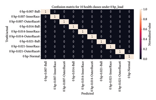
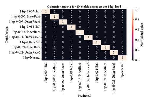
4.4.3.1.2. Visual Analysis of the Model Using a Confusion Matrix. After evaluating the model on the testing dataset, a heatmap of the confusion matrix was generated to visually represent the classification accuracy for 10 health states across four load conditions (0∼3 hp). The matrix exhibited perfect classification, with all 10 health classes achieving a value of one, indicating that the model correctly classified every instance in the testing dataset. Notably, the diagonal elements of the heatmap predominantly displayed values of 1, emphasizing the model’s proficiency in accurately identifying each health class, even in the presence of imbalanced health distributions.
Figure 15 provides a heatmap of the confusion matrix, visually representing model accuracy across 10 health classes under four load conditions, with predicted results on the horizontal axis and actual labels on the vertical axis. This evaluation underscores the robustness and reliability of the 1D-DCNN model in accurately identifying fault conditions within the provided dataset.


4.4.3.1.3. Bearing Diagnosis Utilizing Classification Report Results. In addition to the confusion matrix, a classification report was generated to evaluate precision, recall, and F1-score for each of the 10 health classes under four varying loading conditions (0∼3 hp). The results showcased perfect precision, recall, and F1-score values of 1.00 for all health classes, indicating the model’s remarkable ability to accurately identify each health state. In addition, both macro and weighted average metrics consistently demonstrated excellence, with a value of 1, affirming the reliability and effectiveness of the 1D-DCNN model in bearing fault diagnosis. Table 4 presents the classification report in detail, offering a comprehensive overview of evaluation metrics such as accuracy, precision, recall, and F1-score across four varying load conditions.
| Precision | Recall | F1-score | Support | |
|---|---|---|---|---|
| Classification report for 10 health conditions under 0 hp_load: | ||||
| A | ||||
| 0 hp-0.007-Ball | 1.00 | 1.00 | 1.00 | 62 |
| 0 hp-0.007-InnerRace | 1.00 | 1.00 | 1.00 | 58 |
| 0 hp-0.007-OuterRace6 | 1.00 | 1.00 | 1.00 | 53 |
| 0 hp-0.014-Ball | 1.00 | 1.00 | 1.00 | 65 |
| 0 hp-0.014-InnerRace | 1.00 | 1.00 | 1.00 | 58 |
| 0 hp-0.014-OuterRace6 | 1.00 | 1.00 | 1.00 | 72 |
| 0 hp-0.021-Ball | 1.00 | 1.00 | 1.00 | 61 |
| 0 hp-0.021-InnerRrace | 1.00 | 1.00 | 1.00 | 43 |
| 0 hp-0.021-OuterRrace6 | 1.00 | 1.00 | 1.00 | 58 |
| 0 hp-Normal | 1.00 | 1.00 | 1.00 | 138 |
| Accuracy | 1.00 | 668 | ||
| Macro avg | 1.00 | 1.00 | 1.00 | 668 |
| Weighted avg | 1.00 | 1.00 | 1.00 | 668 |
| Classification report for 10 health conditions under 1 hp_load: | ||||
| B | ||||
| 1 hp-0.007-Ball | 1.00 | 1.00 | 1.00 | 54 |
| 1 hp-0.007-InnerRace | 1.00 | 1.00 | 1.00 | 57 |
| 1 hp-0.007-OuterRace6 | 1.00 | 1.00 | 1.00 | 65 |
| 1 hp-0.014-Ball | 1.00 | 1.00 | 1.00 | 51 |
| 1 hp-0.014-InnerRace | 1.00 | 1.00 | 1.00 | 65 |
| 1 hp-0.014-OuterRace6 | 1.00 | 1.00 | 1.00 | 72 |
| 1 hp-0.021-Ball | 1.00 | 1.00 | 1.00 | 57 |
| 1 hp-0.021-InnerRrace | 1.00 | 1.00 | 1.00 | 59 |
| 1 hp-0.021-OuterRrace6 | 1.00 | 1.00 | 1.00 | 51 |
| 1 hp-Normal | 1.00 | 1.00 | 1.00 | 257 |
| Accuracy | 1.00 | 788 | ||
| Macro avg | 1.00 | 1.00 | 1.00 | 788 |
| Weighted avg | 1.00 | 1.00 | 1.00 | 788 |
| Classification report for 10 health conditions under 2 hp_load: | ||||
| C | ||||
| 2 hp-0.007-Ball | 1.00 | 1.00 | 1.00 | 55 |
| 2 hp-0.007-InnerRace | 1.00 | 1.00 | 1.00 | 62 |
| 2 hp-0.007-OuterRace6 | 1.00 | 1.00 | 1.00 | 53 |
| 2 hp-0.014-Ball | 1.00 | 1.00 | 1.00 | 60 |
| 2 hp-0.014-InnerRace | 1.00 | 1.00 | 1.00 | 73 |
| 2 hp-0.014-OuterRace6 | 1.00 | 1.00 | 1.00 | 45 |
| 2 hp-0.021-Ball | 1.00 | 1.00 | 1.00 | 57 |
| 2 hp-0.021-InnerRrace | 1.00 | 1.00 | 1.00 | 65 |
| 2 hp-0.021-OuterRrace6 | 1.00 | 1.00 | 1.00 | 65 |
| 2 hp-Normal | 1.00 | 1.00 | 1.00 | 253 |
| Accuracy | 1.00 | 788 | ||
| Macro avg | 1.00 | 1.00 | 1.00 | 788 |
| Weighted avg | 1.00 | 1.00 | 1.00 | 788 |
| Classification report for 10 health conditions under 3 hp_load: | ||||
| D | ||||
| 3 hp-0.007-Ball | 1.00 | 1.00 | 1.00 | 53 |
| 3 hp-0.007-InnerRace | 1.00 | 1.00 | 1.00 | 65 |
| 3 hp-0.007-OuterRace6 | 1.00 | 1.00 | 1.00 | 66 |
| 3 hp-0.014-Ball | 1.00 | 1.00 | 1.00 | 68 |
| 3 hp-0.014-InnerRace | 1.00 | 1.00 | 1.00 | 54 |
| 3 hp-0.014-OuterRace6 | 1.00 | 1.00 | 1.00 | 65 |
| 3 hp-0.021-Ball | 1.00 | 1.00 | 1.00 | 76 |
| 3 hp-0.021-InnerRrace | 1.00 | 1.00 | 1.00 | 46 |
| 3 hp-0.021-OuterRrace6 | 1.00 | 1.00 | 1.00 | 69 |
| 3 hp-Normal | 1.00 | 1.00 | 1.00 | 228 |
| Accuracy | 1.00 | 790 | ||
| Macro avg | 1.00 | 1.00 | 1.00 | 790 |
| Weighted avg | 1.00 | 1.00 | 1.00 | 790 |
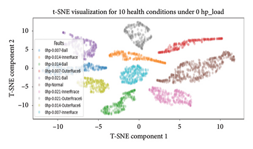
4.4.3.1.4. Dimensional Reduction Utilizing t-SNE for Visualization of Health States. In the final evaluation, t-SNE was used for dimensional reduction. It leveraged the pretrained 1D-DCNN model to extract features from its second-to-last layer, and a new model was created to predict on the training data, capturing abstract representations from this layer. In this work, the thorough analysis extends to deeper layers, particularly the second-to-last layer, where t-SNE’s effectiveness improves as it extracts more discriminative and representative features.
The scatter plot in Figure 16 shows reduced-dimensional data and clustering of bearing health states, grouping similar states together and distinguishing various faults. Different health categories are represented by colors, showcasing the model ability to differentiate and cluster diverse health classes.
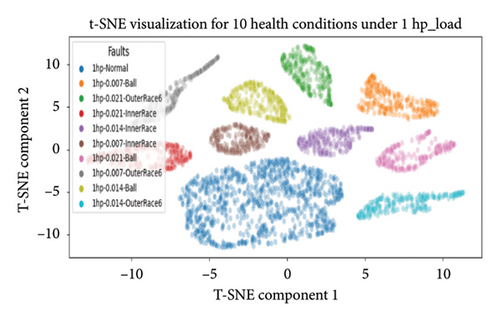
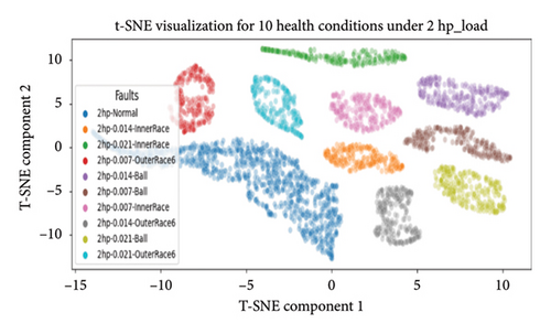
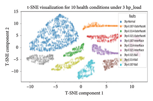
Overall, the 1D-DCNN model demonstrated outstanding performance across the 10 unbalanced health classes and four varying loading conditions (0∼3 hp), as evidenced by all the evaluation metrics discussed. Notably, the model achieved flawless accuracy of 100% on the testing data for each categorized health class, with perfect accuracy, precision, recall, and F1-scores of 1 for every class. This level of accuracy is highly commendable, particularly given imbalanced class distributions across varying load conditions. Hence, the results underscore the 1D-DCNN model effectiveness and robustness in handling unbalanced health states across varying loading conditions.
4.4.3.2. Bearing Diagnosis Results Under Four Different Unbalanced High-Class Health States
In addition, this section presents the outcomes of bearing fault diagnosis for unbalanced high-class health states, including 20, 30, 40, and 64 classes across varying loading conditions (0∼3 hp).
4.4.3.2.1. Bearing Diagnosis Results Utilizing Classification Accuracy Metrics. In line with previous sections of 4.4.3.1, across 20, 30, and 40 high-class health states under different loading conditions, the model consistently improved its performance throughout training, reaching 100% accuracy on both the training and validation sets by the final epoch. This highlights its capability to comprehend and generalize from the training data, enabling accurate diagnosis of bearing faults within the context of unbalanced high-class health states. Likewise, within the realm of 64 health classes, the model showcased effective training performance, reaching a peak training accuracy of 99.95% and sustaining an impressive 99.96% validation accuracy. These results underscore the model capacity to learn and generalize across a wide spectrum of fault conditions encompassed within the 64 health classes. Figure 17 depicts the training progress, showcasing accuracy and loss curves that demonstrate successful model training and the minimization of loss functions across 20, 30, 40, and 64 high-class health states.
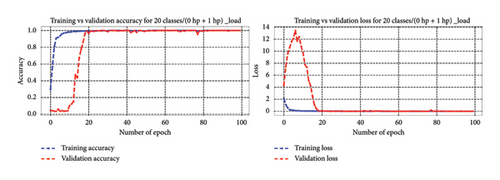
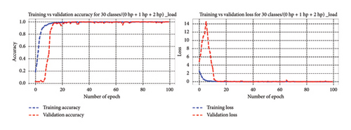
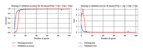
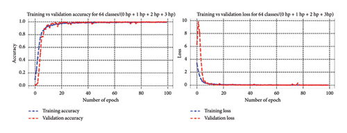
The 1D-DCNN model exhibited strong learning capabilities and achieved high accuracy across all categorized high-class health states. Following training and validation, the 1D-DCNN model underwent testing with test datasets and demonstrated exceptional performance across unbalanced high-class health states of 20, 30, and 40 classes, reaching 100% accuracy and yielding a minimal test loss of 0.0000. Similarly, when evaluated across 64 health classes, it exhibited outstanding performance with a minimal test loss of 0.0036 and an impressive accuracy of 99.96%. These findings underscore the model proficiency in achieving remarkable accuracy and minimal loss on unseen test data, indicating its robust ability to generalize effectively and classify instances.
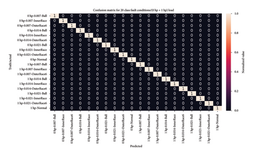
4.4.3.2.2. Visual Analysis of the Model Using a Confusion Matrix. In addition, the model performance was assessed using a heatmap plot to depict the confusion matrix. Notably, it achieved flawless classification for 20, 30, and 40 health classes, with all classes exhibiting a diagonal element of 1, indicating accurate classification of every instance in the test dataset. Likewise, the heatmap plot for 64 high-class health states reveals remarkable performance across all class conditions, with values predominantly close to 1, indicating near-perfect predictions. While two classes exhibit slightly lower values of 0.98 and 0.99, the overall accuracy of the proposed model remains outstanding for high-class health states. Even in cases of misclassification among the 64 health states, the testing accuracy for the four normal classes consistently remains at 1, underscoring the model remarkable and consistent performance.
Figure 18 provides a detailed presentation of the model capabilities through a heatmap plot, offering clear insights into its proficiency across four high-class health states. Hence, these findings highlight the model’s effectiveness and robustness in diagnosing bearing faults under varying load conditions.
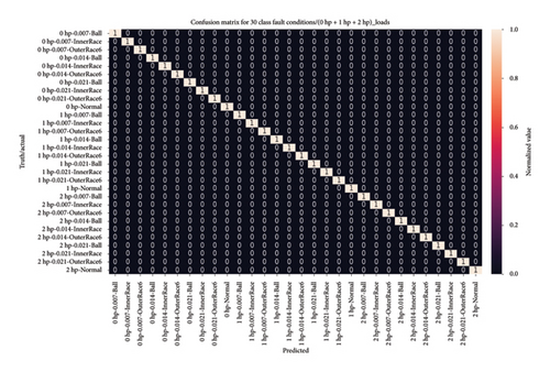
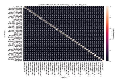
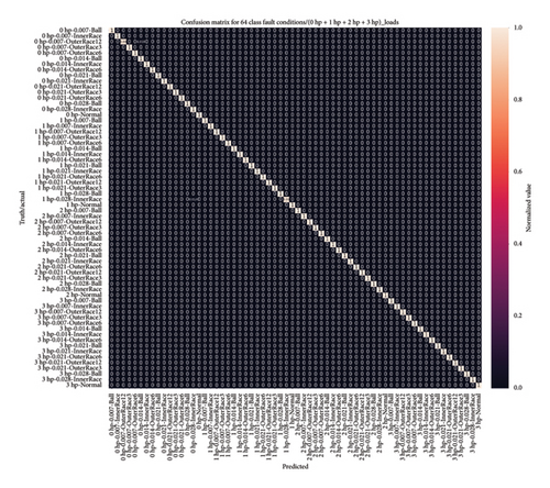
4.4.3.2.3. Bearing Diagnosis Utilizing Classification Report Results. In addition, a detailed classification report highlights outstanding model performance across 20, 30, and 40 health classes, with precision, recall, and F1-scores consistently reaching 1.00 for each class. Moreover, the model performance analysis across 64 health classes under varying load conditions reveals high precision, recall, and F1-scores, with most values near 1, indicating effective health classification. Although two classes have slightly lower scores of 0.98 and 0.99, the overall accuracy for the 64 health states remains outstanding. Table 5 presents a detailed classification report, highlighting evaluation metrics for the 20, 30, 40, and 64 unbalanced high-class health states under varying loading conditions. These results underscore the 1D-DCNN model suitability and efficacy in bearing fault diagnosis, demonstrating remarkable performance across diverse fault and load scenarios.
| Precision | Recall | F1-score | Support | |
|---|---|---|---|---|
| Classification report for 20 health classes/(0 hp + 1 hp)_load: | ||||
| A | ||||
| 0 hp-0.007-Ball | 1.00 | 1.00 | 1.00 | 60 |
| 0 hp-0.007-InnerRace | 1.00 | 1.00 | 1.00 | 64 |
| 0 hp-0.007-OuterRace6 | 1.00 | 1.00 | 1.00 | 68 |
| 0 hp-0.014-Ball | 1.00 | 1.00 | 1.00 | 55 |
| 0 hp-0.014-InnerRace | 1.00 | 1.00 | 1.00 | 55 |
| 0 hp-0.014-OuterRace6 | 1.00 | 1.00 | 1.00 | 54 |
| 0 hp-0.021-Ball | 1.00 | 1.00 | 1.00 | 57 |
| 0 hp-0.021-InnerRrace | 1.00 | 1.00 | 1.00 | 70 |
| 0 hp-0.021-OuterRrace6 | 1.00 | 1.00 | 1.00 | 63 |
| 0 hp-Normal | 1.00 | 1.00 | 1.00 | 114 |
| 1 hp-0.007-Ball | 1.00 | 1.00 | 1.00 | 62 |
| 1 hp-0.007-InnerRace | 1.00 | 1.00 | 1.00 | 61 |
| 1 hp-0.007-OuterRace6 | 1.00 | 1.00 | 1.00 | 52 |
| 1 hp-0.014-Ball | 1.00 | 1.00 | 1.00 | 62 |
| 1 hp-0.014-InnerRace | 1.00 | 1.00 | 1.00 | 64 |
| 1 hp-0.014-OuterRace6 | 1.00 | 1.00 | 1.00 | 61 |
| 1 hp-0.021-Ball | 1.00 | 1.00 | 1.00 | 71 |
| 1 hp-0.021-InnerRrace | 1.00 | 1.00 | 1.00 | 60 |
| 1 hp-0.021-OuterRrace6 | 1.00 | 1.00 | 1.00 | 68 |
| 1 hp-Normal | 1.00 | 1.00 | 1.00 | 235 |
| Accuracy | 1.00 | 1456 | ||
| Macro avg | 1.00 | 1.00 | 1.00 | 1456 |
| Weighted avg | 1.00 | 1.00 | 1.00 | 1456 |
| Classification report for 30 health classes/(0 hp + 1 hp + 2 hp)_load: | ||||
| B | ||||
| 0 hp-0.007-Ball | 1.00 | 1.00 | 1.00 | 50 |
| 0 hp-0.007-InnerRace | 1.00 | 1.00 | 1.00 | 57 |
| 0 hp-0.007-OuterRace6 | 1.00 | 1.00 | 1.00 | 62 |
| 0 hp-0.014-Ball | 1.00 | 1.00 | 1.00 | 54 |
| 0 hp-0.014-InnerRace | 1.00 | 1.00 | 1.00 | 49 |
| 0 hp-0.014-OuterRace6 | 1.00 | 1.00 | 1.00 | 66 |
| 0 hp-0.021-Ball | 1.00 | 1.00 | 1.00 | 66 |
| 0 hp-0.021-InnerRrace | 1.00 | 1.00 | 1.00 | 56 |
| 0 hp-0.021-OuterRrace6 | 1.00 | 1.00 | 1.00 | 56 |
| 0 hp-Normal | 1.00 | 1.00 | 1.00 | 118 |
| 1 hp-0.007-Ball | 1.00 | 1.00 | 1.00 | 64 |
| 1 hp-0.007-InnerRace | 1.00 | 1.00 | 1.00 | 55 |
| 1 hp-0.007-OuterRace6 | 1.00 | 1.00 | 1.00 | 58 |
| 1 hp-0.014-Ball | 1.00 | 1.00 | 1.00 | 57 |
| 1 hp-0.014-InnerRace | 1.00 | 1.00 | 1.00 | 68 |
| 1 hp-0.014-OuterRace6 | 1.00 | 1.00 | 1.00 | 55 |
| 1 hp-0.021-Ball | 1.00 | 1.00 | 1.00 | 62 |
| 1 hp-0.021-InnerRrace | 1.00 | 1.00 | 1.00 | 66 |
| 1 hp-0.021-OuterRrace6 | 1.00 | 1.00 | 1.00 | 63 |
| 1 hp-Normal | 1.00 | 1.00 | 1.00 | 232 |
| 2 hp-0.007-Ball | 1.00 | 1.00 | 1.00 | 58 |
| 2 hp-0.007-InnerRace | 1.00 | 1.00 | 1.00 | 61 |
| 2 hp-0.007-OuterRace6 | 1.00 | 1.00 | 1.00 | 65 |
| 2 hp-0.014-Ball | 1.00 | 1.00 | 1.00 | 61 |
| 2 hp-0.014-InnerRace | 1.00 | 1.00 | 1.00 | 71 |
| 2 hp-0.014-OuterRace6 | 1.00 | 1.00 | 1.00 | 65 |
| 2 hp-0.021-Ball | 1.00 | 1.00 | 1.00 | 73 |
| 2 hp-0.021-InnerRrace | 1.00 | 1.00 | 1.00 | 55 |
| 2 hp-0.021-OuterRrace6 | 1.00 | 1.00 | 1.00 | 65 |
| 2 hp-Normal | 1.00 | 1.00 | 1.00 | 256 |
| Accuracy | 1.00 | 2244 | ||
| Macro avg | 1.00 | 1.00 | 1.00 | 2244 |
| Weighted avg | 1.00 | 1.00 | 1.00 | 2244 |
| Classification report for 40 health classes/(0 hp + 1 hp + 2 hp + 3 hp)_load: | ||||
| C | ||||
| 0 hp-0.007-Ball | 1.00 | 1.00 | 1.00 | 63 |
| 0 hp-0.007-InnerRace | 1.00 | 1.00 | 1.00 | 64 |
| 0 hp-0.007-OuterRace6 | 1.00 | 1.00 | 1.00 | 61 |
| 0 hp-0.014-Ball | 1.00 | 1.00 | 1.00 | 68 |
| 0 hp-0.014-InnerRace | 1.00 | 1.00 | 1.00 | 70 |
| 0 hp-0.014-OuterRace6 | 1.00 | 1.00 | 1.00 | 56 |
| 0 hp-0.021-Ball | 1.00 | 1.00 | 1.00 | 74 |
| 0 hp-0.021-InnerRrace | 1.00 | 1.00 | 1.00 | 44 |
| 0 hp-0.021-OuterRrace6 | 1.00 | 1.00 | 1.00 | 50 |
| 0 hp-Normal | 1.00 | 1.00 | 1.00 | 135 |
| 1 hp-0.007-Ball | 1.00 | 1.00 | 1.00 | 57 |
| 1 hp-0.007-InnerRace | 1.00 | 1.00 | 1.00 | 67 |
| 1 hp-0.007-OuterRace6 | 1.00 | 1.00 | 1.00 | 69 |
| 1 hp-0.014-Ball | 1.00 | 1.00 | 1.00 | 64 |
| 1 hp-0.014-InnerRace | 1.00 | 1.00 | 1.00 | 57 |
| 1 hp-0.014-OuterRace6 | 1.00 | 1.00 | 1.00 | 65 |
| 1 hp-0.021-Ball | 1.00 | 1.00 | 1.00 | 56 |
| 1 hp-0.021-InnerRrace | 1.00 | 1.00 | 1.00 | 51 |
| 1 hp-0.021-OuterRrace6 | 1.00 | 1.00 | 1.00 | 60 |
| 1 hp-Normal | 1.00 | 1.00 | 1.00 | 235 |
| 2 hp-0.007-Ball | 1.00 | 1.00 | 1.00 | 55 |
| 2 hp-0.007-InnerRace | 1.00 | 1.00 | 1.00 | 62 |
| 2 hp-0.007-OuterRace6 | 1.00 | 1.00 | 1.00 | 68 |
| 2 hp-0.014-Ball | 1.00 | 1.00 | 1.00 | 60 |
| 2 hp-0.014-InnerRace | 1.00 | 1.00 | 1.00 | 64 |
| 2 hp-0.014-OuterRace6 | 1.00 | 1.00 | 1.00 | 63 |
| 2 hp-0.021-Ball | 1.00 | 1.00 | 1.00 | 50 |
| 2 hp-0.021-InnerRrace | 1.00 | 1.00 | 1.00 | 74 |
| 2 hp-0.021-OuterRrace6 | 1.00 | 1.00 | 1.00 | 48 |
| 2 hp-Normal | 1.00 | 1.00 | 1.00 | 231 |
| 3 hp-0.007-Ball | 1.00 | 1.00 | 1.00 | 64 |
| 3 hp-0.007-InnerRace | 1.00 | 1.00 | 1.00 | 67 |
| 3 hp-0.007-OuterRace6 | 1.00 | 1.00 | 1.00 | 58 |
| 3 hp-0.014-Ball | 1.00 | 1.00 | 1.00 | 65 |
| 3 hp-0.014-InnerRace | 1.00 | 1.00 | 1.00 | 66 |
| 3 hp-0.014-OuterRace6 | 1.00 | 1.00 | 1.00 | 60 |
| 3 hp-0.021-Ball | 1.00 | 1.00 | 1.00 | 64 |
| 3 hp-0.021-InnerRrace | 1.00 | 1.00 | 1.00 | 70 |
| 3 hp-0.021-OuterRrace6 | 1.00 | 1.00 | 1.00 | 52 |
| 3 hp-Normal | 1.00 | 1.00 | 1.00 | 226 |
| Accuracy | 1.00 | 3033 | ||
| Macro avg | 1.00 | 1.00 | 1.00 | 3033 |
| Weighted avg | 1.00 | 1.00 | 1.00 | 3033 |
| Classification report for 64 health classes/(0 hp + 1 hp + 2 hp + 3 hp) _load: | ||||
| D | ||||
| 0 hp-0.007-Ball | 1.00 | 1.00 | 1.00 | 69 |
| 0 hp-0.007-InnerRace | 1.00 | 1.00 | 1.00 | 67 |
| 0 hp-0.007-OuterRace12 | 0.98 | 1.00 | 0.99 | 60 |
| 0 hp-0.007-OuterRace3 | 1.00 | 1.00 | 1.00 | 61 |
| 0 hp-0.007-OuterRace6 | 1.00 | 1.00 | 1.00 | 58 |
| 0 hp-0.014-Ball | 1.00 | 0.98 | 0.99 | 50 |
| 0 hp-0.014-InnerRace | 1.00 | 1.00 | 1.00 | 56 |
| 0 hp-0.014-OuterRace6 | 1.00 | 1.00 | 1.00 | 70 |
| 0 hp-0.021-Ball | 1.00 | 1.00 | 1.00 | 54 |
| 0 hp-0.021-InnerRrace | 1.00 | 1.00 | 1.00 | 56 |
| 0 hp-0.021-OuterRrace12 | 1.00 | 1.00 | 1.00 | 73 |
| 0 hp-0.021-OuterRrace3 | 1.00 | 1.00 | 1.00 | 62 |
| 0 hp-0.021-OuterRrace6 | 1.00 | 1.00 | 1.00 | 61 |
| 0 hp-0.028-Ball | 1.00 | 1.00 | 1.00 | 49 |
| 0 hp-0.028-InnerRace | 1.00 | 0.98 | 0.99 | 54 |
| 0 hp-Normal | 1.00 | 1.00 | 1.00 | 113 |
| 1 hp-0.007-Ball | 1.00 | 1.00 | 1.00 | 61 |
| 1 hp-0.007-InnerRace | 1.00 | 1.00 | 1.00 | 60 |
| 1 hp-0.007-OuterRace12 | 1.00 | 1.00 | 1.00 | 57 |
| 1 hp-0.007-OuterRace3 | 1.00 | 1.00 | 1.00 | 59 |
| 1 hp-0.007-OuterRace6 | 1.00 | 1.00 | 1.00 | 61 |
| 1 hp-0.014-Ball | 1.00 | 1.00 | 1.00 | 69 |
| 1 hp-0.014-InnerRace | 1.00 | 1.00 | 1.00 | 61 |
| 1 hp-0.014-OuterRace6 | 1.00 | 1.00 | 1.00 | 68 |
| 1 hp-0.021-Ball | 1.00 | 1.00 | 1.00 | 58 |
| 1 hp-0.021-InnerRace | 1.00 | 1.00 | 1.00 | 56 |
| 1 hp-0.021-OuterRace6 | 1.00 | 1.00 | 1.00 | 59 |
| 1 hp-0.021-OuterRrace12 | 1.00 | 1.00 | 1.00 | 59 |
| 1 hp-0.021-OuterRrace3 | 1.00 | 1.00 | 1.00 | 68 |
| 1 hp-0.028-Ball | 1.00 | 1.00 | 1.00 | 56 |
| 1 hp-0.028-InnerRace | 0.99 | 1.00 | 0.99 | 68 |
| 1 hp-Normal | 1.00 | 1.00 | 1.00 | 245 |
| 2 hp-0.007-Ball | 1.00 | 1.00 | 1.00 | 69 |
| 2 hp-0.007-InnerRace | 1.00 | 1.00 | 1.00 | 54 |
| 2 hp-0.007-OuterRace12 | 1.00 | 1.00 | 1.00 | 70 |
| 2 hp-0.007-OuterRace3 | 1.00 | 1.00 | 1.00 | 54 |
| 2 hp-0.007-OuterRace6 | 1.00 | 1.00 | 1.00 | 69 |
| 2 hp-0.014-Ball | 1.00 | 1.00 | 1.00 | 63 |
| 2 hp-0.014-InnerRace | 1.00 | 1.00 | 1.00 | 61 |
| 2 hp-0.014-OuterRace6 | 1.00 | 1.00 | 1.00 | 61 |
| 2 hp-0.021-Ball | 1.00 | 1.00 | 1.00 | 53 |
| 2 hp-0.021-InnerRace | 1.00 | 1.00 | 1.00 | 62 |
| 2 hp-0.021-OuterRace6 | 1.00 | 1.00 | 1.00 | 65 |
| 2 hp-0.021-OuterRrace12 | 1.00 | 1.00 | 1.00 | 66 |
| 2 hp-0.021-OuterRrace3 | 1.00 | 1.00 | 1.00 | 59 |
| 2 hp-0.028-Ball | 1.00 | 1.00 | 1.00 | 59 |
| 2 hp-0.028-InnerRace | 1.00 | 1.00 | 1.00 | 54 |
| 2 hp-Normal | 1.00 | 1.00 | 1.00 | 242 |
| 3 hp-0.007-Ball | 1.00 | 1.00 | 1.00 | 55 |
| 3 hp-0.007-InnerRace | 1.00 | 1.00 | 1.00 | 63 |
| 3 hp-0.007-OuterRace12 | 1.00 | 1.00 | 1.00 | 66 |
| 3 hp-0.007-OuterRace3 | 1.00 | 1.00 | 1.00 | 58 |
| 3 hp-0.007-OuterRace6 | 1.00 | 1.00 | 1.00 | 59 |
| 3 hp-0.014-Ball | 1.00 | 1.00 | 1.00 | 67 |
| 3 hp-0.014-InnerRace | 1.00 | 1.00 | 1.00 | 70 |
| 3 hp-0.014-OuterRace6 | 1.00 | 1.00 | 1.00 | 62 |
| 3 hp-0.021-Ball | 1.00 | 1.00 | 1.00 | 61 |
| 3 hp-0.021-InnerRace | 1.00 | 1.00 | 1.00 | 54 |
| 3 hp-0.021-OuterRace6 | 1.00 | 1.00 | 1.00 | 56 |
| 3 hp-0.021-OuterRrace12 | 1.00 | 1.00 | 1.00 | 64 |
| 3 hp-0.021-OuterRrace3 | 1.00 | 1.00 | 1.00 | 63 |
| 3 hp-0.028-Ball | 1.00 | 1.00 | 1.00 | 60 |
| 3 hp-0.028-InnerRace | 1.00 | 1.00 | 1.00 | 58 |
| 3 hp-Normal | 1.00 | 1.00 | 1.00 | 232 |
| Accuracy | 1.00 | 4487 | ||
| Macro avg | 1.00 | 1.00 | 1.00 | 4487 |
| Weighted avg | 1.00 | 1.00 | 1.00 | 4487 |
4.4.3.2.4. Dimensional Reduction Utilizing t-SNE for Visualization of High-Class Health States. Moreover, a pretrained CNN with t-SNE dimensionality reduction effectively captured feature representations from the second-to-last layer, achieving excellent predictions for 20, 30, 40, and 64 health classes. The visualization, depicted in Figure 19 as a scatter plot, effectively illustrates the model performance in representing 20, 30, 40, and 64 high-class health states under various loading conditions within a reduced-dimensional space. Each point on the plot corresponds to a health condition, providing insights into the model ability to differentiate and cluster the diverse set of health classes. Hence, this visual representation significantly contributes to the comprehensive evaluation of the 1D-DCNN model performance, confirming its effectiveness and robustness across four distinct unbalanced high-class health states.
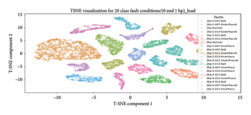
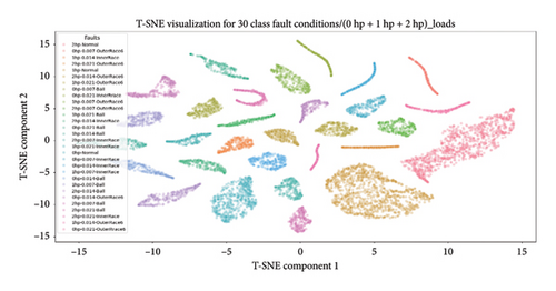
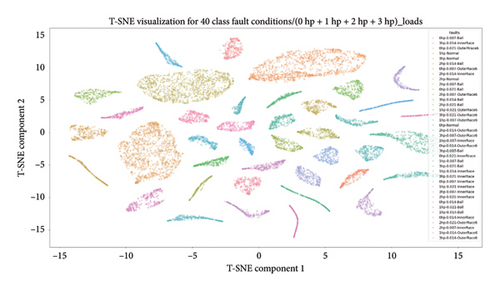
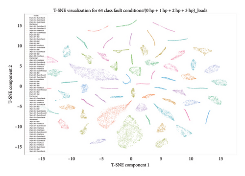
Overall, the 1D-DCNN model demonstrates outstanding performance on imbalanced high-class health states, achieving remarkable results for 20, 30, and 40 classes under four different loading conditions, with 100% accuracy on the testing data. In addition, the model achieves perfect accuracy, precision, recall, and F1-scores of 1 for each high-class health state. Moreover, the model shows remarkable capabilities on 64 unbalanced high-class health states, achieving near-perfect precision, recall, and F1-scores, with the majority of health classes attaining a score of 1. Despite minor variations, such as two classes showing slightly lower values of 0.98 and 0.99, the overall performance and accuracy of the model across all classes remain impressive, given the increased complexity and greater diversity of health classes. Hence, the proposed 1D-DCNN model outstanding performance across all categorized high-class health states highlights its robustness and effective accuracy across diverse health and varying load conditions.
4.5. Comparison With Other State-of-The-Art CNN-Based Diagnostic Methods
To demonstrate the superiority of the proposed 1D-DCNN and enhance the reliability of the diagnostic results, this study compares it with several advanced state-of-the-art CNN models. The primary selection criteria aimed to ensure continuity in research and address the existing gap. Comparative models were selected based on the similarity of their datasets to the proposed method, with all training and testing conducted on the CWRU motor bearing dataset across varying load conditions (0∼3 hp). In additionally, the model architecture had to exhibit somewhat similar behavior, and the research had to be recent.
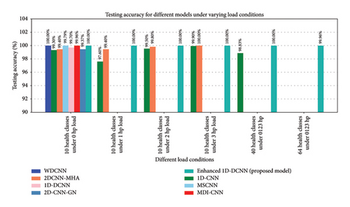
Based on the provided criteria, the selected models comprise seven advanced state-of-the-art methods, including 1D-CNN and 2D-CNN, each offering unique techniques for bearing fault diagnosis. These models include deep convolutional neural networks with wide first-layer kernels (WDCNN) [38], 1D-CNNs with dropout operations [5], two-dimensional convolutional neural network with multi-head attention mechanism (2DCNN-MHA) [28], multiscale convolutional neural network (MSCNN) [47], 1D-DCNN [51], multidimension input convolutional neural network (MDI-CNN) [40], and two-dimensional convolutional neural network with group normalization (2D-CNN-GN) [7]. The diagnostic performance of these comparative models covered six categorized health classes across varying load conditions, including 0∼3 hp for 10 health states, as well as 40 and 64 high-class health states. The average fault diagnosis testing accuracies of the comparative methods are detailed in Table 6.
| No | Models and references | Testing accuracy for six different categorized health classes under varying loading conditions | |||||
|---|---|---|---|---|---|---|---|
| 10 health classes under 0 hp load | 10 health classes under 1 hp load | 10 health classes under 2 hp load | 10 health classes under 3 hp load | 40 health classes under combined 0∼3 hp loads | 64 health classes under combined 0∼3 hp loads | ||
| 1 | WDCNN [38] | 100 | — | — | — | — | — |
| 2 | 1D-CNN [5] | 99.3 | 97.6 | 99.5 | 99.9 | 98.83 | — |
| 3 | 2DCNN-MHA [28] | 99.4 | 99.4 | 99.8 | 100 | — | — |
| 4 | MSCNN [47] | 99.79 | — | — | — | — | — |
| 5 | 1D-DCNN [51] | 99.70 | — | — | — | — | — |
| 6 | MDI-CNN [40] | 99.96 | — | — | — | — | — |
| 7 | 2D-CNN-GN [7] | 99.37 | — | — | — | — | — |
| 8 | Enhanced 1D-DCNN (proposed method) | 100 ± 0 | 100 ± 0 | 100 ± 0 | 100 ± 0 | 100 ± 0 | 99.96 ± 0.0002 |
As presented in Table 6, the proposed enhanced 1D-DCNN method exhibits superior performance across 10 bearing health states under various working and loading conditions (0∼3 hp) compared with existing approaches. Notably, existing bearing fault diagnosis methods based on 1D-CNN and 2D-CNN often assume balanced training data for each bearing health state, frequently resorting to data augmentation techniques. However, such an approach can result in prolonged processing times, heightened costs or resource usage, and potential information loss in the raw dynamic data. In contrast, our proposed method directly utilizes unbalanced bearing health states obtained from the CWRU bearing datasets. This choice is motivated by the reality that in real-world scenarios, bearing faults are infrequent while healthy data is abundant, making it impractical to gather extensive fault signals. By addressing this challenge, our proposed approach fills a significant gap left by existing methods, effectively diagnosing each health state within unbalanced scenarios without the need for data augmentation techniques.
While the testing accuracy of the WDCNN and 2DCNN-MHA methods in Table 6 may appear comparable to our proposed method under 0 and 3 hp loads, respectively, the key distinction lies in the imbalance of classes within our approach, achieved without resorting to data augmentation. This underscores the effectiveness, stability, and robustness of our approach compared to the WDCNN, 2DCNN-MHA, and other state-of-the-art methods. In addition, in the WDCNN method, the model performance was evaluated under a single load condition, whereas our proposed method extended to assessing unbalanced health states and high-class health states across four varying loading conditions. Although some prior studies have achieved diagnostic accuracy close to that of the proposed method, the 1D-DCNN model attains a stable high accuracy with significantly fewer iterations than existing approaches. Moreover, its training and validation curves exhibit a smooth and consistent pattern, confirming the absence of overfitting or underfitting. This improved stability and faster convergence can be attributed to the strategic incorporation of BN and dropout operations. To confirm the robustness of the proposed method, an extensive ablation study was conducted to evaluate the influence of key network parameters and training hyperparameters on the model performance. Consequently, the proposed 1D-DCNN ensures enhanced training efficiency, leading to reliable and consistent diagnostic performance during testing.
Furthermore, in real-world scenarios, bearings encounter a broader range of fault conditions due to diverse operating conditions, including variations in speeds and loads. Therefore, the efficacy of the proposed method is demonstrated not only under the specified 10 unbalanced bearing health states across four varying load conditions but also when handling an expanded number of categorized unbalanced high-class health states. Specifically, it achieves a flawless score of 100% across 40 health states. In addition, the method extends its effectiveness to 64 health states under combined 0∼3 hp loads, showcasing remarkable performance with a testing accuracy reaching 99.96%. These findings underscore the favorable and robust nature of the proposed method when compared with existing approaches. In Figure 20, the average testing accuracy for bearing health state classification is depicted, facilitating a comparative analysis between the proposed method and other state-of-the-art methods. This visualization provides valuable insights into the accuracy of different models under various loading conditions.
5. Conclusions
In this study, an enhanced 1D-DCNN fault diagnosis framework was proposed for REBs to address challenges such as limited data, class imbalance, and high-class health states. The method initially employed a continuous segmentation process, using a window stride technique to convert raw 1D vibration signals into segmented samples, leveraging segmentation for feature extraction and 1D-DCNN for health classification. This approach prevents information loss, reduces resource costs, and minimizes processing time. The effectiveness of the method was validated using benchmark data from the CWRU rolling bearing dataset through systematic evaluation across two main groups. First, datasets were categorized into health states under four load levels (0∼3 hp), each comprising 10 unbalanced health states. Second, classification was performed into four unbalanced high-class health categories: 20, 30, 40, and 64 health classes, across the varying load conditions.
Experimental results confirmed the model effectiveness, achieving 100% diagnostic accuracy across 10 unbalanced health classes under all 0∼3 hp loads. In addition, for unbalanced high-class health states (20, 30, and 40 health classes), the model maintained 100% accuracy. Even with the increased complexity of 64 health states, it achieved a peak accuracy of 99.96%. These findings emphasize the model outstanding effectiveness, robustness, and stability in feature extraction and generalization under both unbalanced and high-class health states. Furthermore, the enhanced 1D-DCNN model demonstrated superior performance compared to existing state-of-the-art CNN-based diagnostic methods.
- 1.
The accuracy of bearing fault diagnosis is enhanced through optimizations in both the model network architecture and training hyperparameters. This is achieved by employing a simplified convolutional layer structure comprising three layers and a smaller size of the convolution kernels. In addition, a reduction in dense layers is implemented, featuring smaller neuron counts for each layer.
- 2.
In addition, the accuracy of bearing fault diagnosis is improved by integrating both BN and dropout layers in the 1D-DCNN model. Both layers are incorporated into each convolutional layer, and a dropout operation is also implemented in the dense layer. This integration effectively improves the accuracy of fault diagnosis under unbalanced health and high-class health states across different loads, consequently enhancing the model generalization ability.
- 3.
This proposed approach has robust feature extraction and classification capabilities, particularly in scenarios involving unbalanced health and high-class health states across four varying loading conditions. To complement these strengths, the proposed methods incorporate additional evaluation metrics, such as classification reports that include precision, recall, and F1-score. In addition, this performance is achieved without the use of data augmentation techniques, such as generative models.
In the present work, the effectiveness of the proposed method is validated via motor bearing datasets. In the future, therefore, the authors plan to validate the effectiveness of the method using data from other rotating machines under unbalanced health and high-class health states. In addition, the approach will incorporate condition monitoring data alongside vibration signals to enhance diagnostic performance and reliability for real-world applications.
Conflicts of Interest
The authors declare no conflicts of interest.
Funding
No funding was received for this research.
Open Research
Data Availability Statement
The data that support the findings of this study are available from the corresponding author upon reasonable request.


