Structural Control and Health Monitoring

Volume 2025, Issue 1 6047080

Research Article

Open Access

Active Learning–Enhanced Ensemble Method for Spatiotemporal Correlation Modeling of Neighboring Bridge Behaviors to Girder Overturning

Ru An

Shenzhen Urban Transport Planning Center Co., Ltd. , Shenzhen , Guangdong, 518057 , China

University of Electronic Science and Technology of China , Chengdu , Sichuan, 611731 , China , uestc.edu.cn

Shenzhen Institute for Advanced Study , University of Electronic Science and Technology of China , Shenzhen , Guangdong, 518110 , China , uestc.edu.cn

Search for more papers by this author

Mengjin Sun,

Mengjin Sun

orcid.org/0009-0003-6045-192X

Shanghai Key Laboratory of Engineering Structure Safety , Shanghai Research Institute of Building Sciences Co. Ltd. , Shanghai , 200032 , China

Shanghai Research Institute of Building Sciences Co. Ltd. , 75 Wanping Rd., Shanghai , 200032 , China

Search for more papers by this author

You Dong,

You Dong

orcid.org/0000-0002-2499-0999

Department of Civil and Environmental Engineering , The Hong Kong Polytechnic University , Hong Kong , 999077 , China , polyu.edu.hk

Search for more papers by this author

Lu Guo,

Lu Guo

Shenzhen Urban Transport Planning Center Co., Ltd. , Shenzhen , Guangdong, 518057 , China

Search for more papers by this author

Lei Jia,

Lei Jia

Shenzhen Urban Transport Planning Center Co., Ltd. , Shenzhen , Guangdong, 518057 , China

University of Electronic Science and Technology of China , Chengdu , Sichuan, 611731 , China , uestc.edu.cn

Shenzhen Institute for Advanced Study , University of Electronic Science and Technology of China , Shenzhen , Guangdong, 518110 , China , uestc.edu.cn

Search for more papers by this author

Xiaoming Lei,

Corresponding Author

Xiaoming Lei

orcid.org/0000-0003-0963-3237

Department of Civil and Environmental Engineering , The Hong Kong Polytechnic University , Hong Kong , 999077 , China , polyu.edu.hk

Search for more papers by this author

Ru An,

Ru An

Shenzhen Urban Transport Planning Center Co., Ltd. , Shenzhen , Guangdong, 518057 , China

University of Electronic Science and Technology of China , Chengdu , Sichuan, 611731 , China , uestc.edu.cn

Shenzhen Institute for Advanced Study , University of Electronic Science and Technology of China , Shenzhen , Guangdong, 518110 , China , uestc.edu.cn

Search for more papers by this author

Mengjin Sun,

Mengjin Sun

orcid.org/0009-0003-6045-192X

Shanghai Key Laboratory of Engineering Structure Safety , Shanghai Research Institute of Building Sciences Co. Ltd. , Shanghai , 200032 , China

Shanghai Research Institute of Building Sciences Co. Ltd. , 75 Wanping Rd., Shanghai , 200032 , China

Search for more papers by this author

You Dong,

You Dong

orcid.org/0000-0002-2499-0999

Department of Civil and Environmental Engineering , The Hong Kong Polytechnic University , Hong Kong , 999077 , China , polyu.edu.hk

Search for more papers by this author

Lu Guo,

Lu Guo

Shenzhen Urban Transport Planning Center Co., Ltd. , Shenzhen , Guangdong, 518057 , China

Search for more papers by this author

Lei Jia,

Lei Jia

Shenzhen Urban Transport Planning Center Co., Ltd. , Shenzhen , Guangdong, 518057 , China

University of Electronic Science and Technology of China , Chengdu , Sichuan, 611731 , China , uestc.edu.cn

Shenzhen Institute for Advanced Study , University of Electronic Science and Technology of China , Shenzhen , Guangdong, 518110 , China , uestc.edu.cn

Search for more papers by this author

Xiaoming Lei,

Corresponding Author

Xiaoming Lei

orcid.org/0000-0003-0963-3237

Department of Civil and Environmental Engineering , The Hong Kong Polytechnic University , Hong Kong , 999077 , China , polyu.edu.hk

Search for more papers by this author

First published: 12 May 2025

https://doi.org/10.1155/stc/6047080

Academic Editor: Łukasz Jankowski

Share a link

Email
Wechat
Bluesky

Abstract

Structural health monitoring (SHM) systems are widely deployed in transportation networks, yet traditional methods often focus on individual bridges, overlooking interdependencies between neighboring structures. This study proposes an active learning–enhanced ensemble learning model to predict the tilt behavior of adjacent bridges by leveraging critical response data from multiple bridges. The ensemble model integrates gradient boosting, random forest, and Gaussian process regressors, providing both predictive means and uncertainty quantification. Active learning iteratively selects the most informative samples, improving model efficiency and reducing data requirements. The model accurately predicts vertical displacement and tilt using responses from neighboring bridges, effectively capturing spatiotemporal correlations and dynamic interactions. Active learning achieves comparable accuracy with just 50% of traditional training samples, demonstrating its efficiency. The results reveal structural interdependencies influenced by stiffness and load distribution variations. The successful prediction of tilt behavior underscores the model’s potential for real-time SHM, early overturning warnings, and enhanced bridge safety.

1. Introduction

Bridge structures play a crucial role in transportation infrastructure, ensuring the efficient movement of people and goods, but prolonged use makes them susceptible to damage [1–3]. In recent years, structural health monitoring (SHM) systems have become essential tools for maintaining the structural performance of bridges [4–6]. These systems continuously collect data on various structural responses, which contain huge information for structural performance [7, 8]. Ensuring the structural safety and reliability of grouped bridges based on this vast amount of data remains a paramount concern for engineers and transportation stakeholders [9].

Traditional SHM methods often focus on single-bridge monitoring and overlook dynamic interactions between neighboring structures. Existing models also struggle with generalization, interpretability, and uncertainty quantification, limiting their applicability in safety-critical scenarios. A key gap is the lack of spatiotemporal correlation modeling, where most studies treat each bridge independently [10–12]. Understanding these spatiotemporal correlations is critical for developing robust predictive models that can provide early warnings of structural issues and optimize maintenance strategies.

The increasing prevalence of overloaded traffic exacerbates the risk of girder overturning for ramps in overpasses, particularly for single-column bridges [13, 14]. This situation presents significant safety hazards and potential structural failures [15–17]. To address these challenges, SHM systems are capable of continuously monitoring loads and responses [18]. Typically, they monitor girder lateral inclinations [19], support reactions, and vertical displacements on both sides [20], offering real-time data to issue warnings and swiftly implement mitigation measures. Dan et al. [21] utilized field data from displacement gauges near the bearings to calculate the girder attitude and subsequently introduced a time-varying reliability analysis method for assessing bridge overturning risk. Unlike directly monitoring vertical displacement, the relative displacement of two girder sides can also be indirectly measured using accelerometers, strain gauges, or inclinometers [18, 22]. Chang and Kim [23] placed fiber Bragg grating strain gauges in a seismic bearing and used its stress–strain curve to estimate the support reaction for structural performance assessment. In the bridge network, detecting potential overturning risks in preceding spans or bridges is more beneficial.

The spatiotemporal correlations are critical for predicting responses and assessing the performance of one bridge from neighboring bridges. Cao and Liu [10] proposed a deep learning–based damage localization method for grouped bridges using spatiotemporal correlation of strain data and established a damage localization index. Cao et al. [11] focused on the grouped medium- and small-span bridges to design a probabilistic method to calculate responses and determine damages utilizing acceleration data. Xu et al. [24] identified suspenders tension based on spatiotemporal correlation between girder strain and suspenders tension using a stacked denoising autoencoder and convolutional neural network–based long short-term memory model to construct the correlation model. Lei et al. [25] established the U-Net model to identify regional spatiotemporal correlations from the inspection reports of grouped bridges. Similarly, Liu and Zhang [26] extracted the spatiotemporal correlations of bridges and their associated components from the national bridge inventory database.

Facing with the vast amount of data from various grouped bridges, employing machine learning (ML) technique proves effective in identifying spatiotemporal correlations and predicting responses [27–32]. Ensemble learning (EL) is a powerful method to aggregate several weak ML predictors for detecting hidden features of data and regress targets. In the field of SHM, many EL methods have been applied to make structural performance prediction and assessment [33]. Han et al. [34] stacked five heterogeneous ML models into an EL model to predict natural frequencies from environmental data and effectively detect potential damage in space grid steel structures by statistically analyzing prediction residuals and mitigating environmental influences. Sun et al. [35] presented a data-driven approach using an EL model to predict cable vibration amplitudes based on environmental loads and demonstrated the superior performance of the gradient boosting decision tree (GBDT). Yaghoubzadehfard et al. [36] applied advanced ML techniques, including random forest, GBDT, and XGBoost, to detect bridge damage by analyzing changes in modal parameters, demonstrating the efficacy of these models, particularly random forest, in identifying damage location and severity.

Active learning (AL) is a pattern recognition algorithm that can achieve greater performance, using fewer training labels, with itself selecting the data from which it learns. The goal is to learn a mapping from observations to labels. Most AL techniques are used in structural reliability analysis to enhance the efficiency and accuracy of predicting failure probabilities and assessing structural performance under uncertainty [37, 38]. Dang et al. [39] introduced Bayesian AL to improve precision and efficiency in exacting posterior variance of the failure probability. Zhou et al. [40] designed a new look-ahead learning function for AL to reduce the computational burden achieved by deducing a closed-form expression for the inner integral. Seldom research is used with AL in SHM-based structural assessment [41]. Bull et al. [42, 43] introduced cluster-adaptive AL to address the issue of the absence of diagnostic labels for SHM, showcasing its effectiveness through experiments. Hughes et al. [44] proposed a risk-based AL approach that queries class-label information based on its expected value, demonstrated with a benchmark, showing improved decision-making performance. Zhu et al. [45] proposed an AL for Bayesian deep neural networks to predict the remaining useful life of a battery of limited run-to-failure data by actively selecting samples for labeling.

The contributions of this work can be summarized as follows: (1) The research demonstrates the effectiveness of a surrogate data-driven model in accurately and efficiently predicting the tilt behavior and displacement of adjacent bridges, capturing the spatiotemporal correlations between their responses. (2) The study successfully applies the copula theory to model the dependence structures between different response variables, providing valuable insights into their interdependencies. (3) By employing AL, the model’s performance is significantly improved, particularly in the early stages of training, resulting in a more accurate and efficient prediction model.

The study’s structure is outlined as follows. Section 2 presents the proposed framework for AL-enhanced EL modeling of critical responses among neighboring bridges based on SHM data, involving three main stages. Section 3 provides detailed insight into the EL and AL techniques utilized. Section 4 describes the grouped bridge and its responses, along with copula-based probabilistic modeling to reveal correlations. Section 5 illustrates the model training, AL’s enhancement on predictions, and girder tilt displacement prediction, while Section 6 draws conclusions.

2. General Framework of AL-Enhanced EL for Response Modeling

Figure 1 illustrates a comprehensive framework that integrates AL with EL to model and predict the spatiotemporal responses of neighboring bridges. This framework leverages SHM data to enhance the predictive accuracy and efficiency of the model. Three key components in the framework are SHM data preparation, AL-enhanced EL model training, and prediction responses with uncertainty of neighboring bridges.

Details are in the caption following the image — **Figure 1**
Open in figure viewer PowerPoint

Overall framework for joint probabilistic modeling of responses.

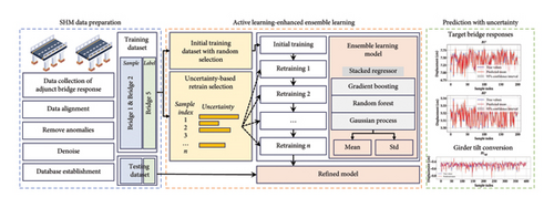
SHM systems are deployed on neighboring bridges to collect critical response data. Data preprocessing involves cleaning the data by removing noise and outliers and handling missing values to ensure high-quality inputs for modeling. A random selection of samples from the collected data forms the training and testing datasets. The training dataset contains the initial training set and the remaining selected by AL strategy for increment training the model. The testing dataset is used to evaluate the model’s performance.

The EL model is established with the stack of gradient boosting regressor, random forest regressor, and Gaussian process regressor. It contains boosting and bagging ensemble algorithms to make use of their advantages. The last stacked regressor with Gaussian process regression could offer a probabilistic approach to regression, capturing uncertainties in predictions, and output standard deviations of predictions for aiding the AL strategy to determine the uncertainties. The uncertainty sampling strategy is based on an entropy-based approach, where predictive variance from the regressor serves as the key criterion for selection. At each iteration, samples with the highest predictive variance are prioritized for labeling and retraining, ensuring that the model efficiently refines its predictions with minimal data.

With the fine-tuned model, the responses of a bridge can be accurately predicted based on data from neighboring bridges. The model successfully extracts and determines the spatiotemporal correlations between neighboring bridges. Comparing the predicted values with the actual measurements demonstrates the model’s accuracy. The predicted mean and 95% confidence intervals are plotted alongside the true values, showcasing the model’s capability to capture the actual behavior of the bridges.

Predicting structural behavior using data from nearby bridges offers several advantages, including faster real-time responses, improved data reliability, and better insights into structural interdependencies. By leveraging spatiotemporal correlations, this approach enables early detection of issues, such as girder overturning, before failure occurs. It also helps fill in gaps caused by sensor failures or data loss, ensuring continuous monitoring.

3. Details of EL and AL

3.1. EL Methods

EL is a powerful technique in ML that involves stacking multiple models to achieve better predictive performance than any single model could on its own. The fundamental idea is that by aggregating the predictions of several models, the ensemble can mitigate the weaknesses of individual models and improve overall accuracy, robustness, and generalization.

EL methods, such as boosting and bagging, are powerful techniques used to improve the accuracy and robustness of ML models. The final prediction is made by averaging the predictions for regression. Boosting methods are trained sequentially, each new model focusing on correcting the errors of the previous ones. This is achieved by adjusting the weights of the training samples based on the errors. Bagging methods, known as bootstrap aggregating, are trained independently on different random subsets of the training data, created through bootstrapping (random sampling with replacement).

This study introduces a novel EL model by combining three regressors: gradient boosting regressor, random forest regressor, and Gaussian process regressor. The stacking process involves two stages: the base models and the meta-model. The base models, which include the gradient boosting regressor and random forest regressor, are trained in parallel. Each base regressor operates independently, allowing for simultaneous training. Once the base models are trained, their predictions serve as input features for the meta-model, which, in this study, is the Gaussian process regressor. The meta-model is then trained sequentially on these predictions. Figure 2 shows the flowchart of the proposed EL methods.

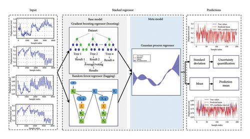
While the base model training is parallelized, the meta-model training occurs sequentially, as it relies on the output from the base models. The gradient boosting regressor and random forest regressor form the foundation of the base model. Gradient boosting regressor is a powerful boosting-based algorithm that sequentially improves weak learners to minimize prediction errors. It is well suited for handling structured SHM data with potential noise and missing values, as it iteratively refines predictions by focusing on difficult-to-model patterns. Random forest regressor is a bagging-based algorithm that builds multiple decision trees in parallel and averages the outputs to improve prediction stability. It is highly effective in reducing variance and capturing feature interactions without requiring extensive hyperparameter tuning.

The Gaussian process regressor, used in the final layer as the meta-model, provides a probabilistic approach to capturing uncertainties in predictions. Gaussian process regressor provides a probabilistic approach to regression, offering uncertainty quantification in predictions. It is particularly useful in AL, as it enables the selection of the most informative samples by evaluating prediction confidence.

For an ensemble to be effective, these base models are diverse, meaning they should make different types of errors. This diversity ensures that the strengths of some models can compensate for the weaknesses of others.

3.1.1. Gradient Boosting Regression

Gradient boosting regressor is a powerful ML technique used for regression tasks. It builds an ensemble of weak decision trees in a sequential manner. Each subsequent tree is trained to correct the errors made by the previous trees, thereby improving the overall performance of the ensemble. Gradient boosting uses gradient descent to minimize the loss function. Each new model is trained to predict the negative gradient of the loss function with respect to the current predictions.

The initial model of the gradient boosting regressor is shown in equation (1). The goal is to find a constant prediction γ that minimizes the initial loss function L(y_i, γ) over all training instances. The loss function L(y_i, γ) represents the loss function that measures the mean-squared error (MSE) between the true value y_i and the predicted value

. The residuals

in the m th weak learner are calculated in equation (2), where the gradient (∂L(y_i, F(x_i))/∂F(x_i)) measures how the loss changes with respect to the current prediction F(x_i). The negative of this gradient represents the direction in which we need to adjust the predictions to reduce the loss.

()

To reduce the prediction error, a new decision tree should be trained to predict the residuals calculated in the previous step, as shown in equation (3). This weak learner h_m(x) is usually a simple model like a shallow decision tree that can quickly fit the residuals

. The previous model F_m−1(x) is the current ensemble model before adding the new weak learner with the certain learning rate η that controls the contribution of the new weak learner. In equation (4), F_M(x) is the updated model that combines the previous model with the scaled predictions of the new weak learner. The final gradient boosting regressor is the aggregate of the initial model and all subsequent updates from the weak learners with equation (5).

()

3.1.2. Random Forest Regression

Another EL aggregate method of weak learners is bagging. Random forest regressor is an EL method that bags multiple decision trees during training and outputs the average prediction of the individual trees for regression tasks. This method improves predictive accuracy and controls overfitting by leveraging the collective power of multiple trees.

Random forest regressor mainly reduces the variance, which refers to the sensitivity of a model to changes in the training data. The variance within a node T is the average squared difference between the actual values y_i and the mean value

. It quantifies the spread of the target values within the node, as shown in equation (6). The critical issue in random forest regressor modeling is the split trees. To find the best Split, evaluate all possible splits. The optimal split minimizes the weighted sum of the variances of the left and right child nodes. The weights are the proportions of instances in the child nodes:

()

where n_L and n_R denote the number of child nodes in the left and right. n denotes the total node numbers in the layer. Var(T_L) and Var(T_R) denote the variances of the left and right child nodes.

At each split in the decision tree, randomly select m features from the total M features. The best split is determined from this subset, which introduces randomness and reduces correlation among trees, as shown in equation (8). The final prediction

is the average of the predictions from all B trees in the forest. This aggregation helps in reducing variance and improving the robustness of the model:

()

3.1.3. Gaussian Process Regression

Gaussian process regressor is a nonparametric Bayesian regression model for modeling complex relationships between input variables and their corresponding continuous output variables. It is based on the concept of modeling the joint distribution of the data using Gaussian processes, which allows for flexible and probabilistic regression predictions. The radial basis function kernel is selected for Gaussian process regression since it effectively captures smooth, nonlinear relationships in the data, including complex spatiotemporal correlations. Additionally, it improves the Gaussian process’s ability to deliver realistic uncertainty estimates, which is essential for AL.

The prior distribution defines the behavior of the Gaussian process before observing any data. Equation (10) specifies that the function values f(x) are drawn from a Gaussian process

with a mean function m(x) and a covariance function k(x, x^′) between inputs x and x^′. Given observed data f and test inputs f_∗, the joint distribution of observed and predicted function values is a multivariate Gaussian with vector mean m and covariance matrix K, as shown in equation (11):

()

Equation (12) shows that the predictive distribution of the test outputs f_∗ given training data (X, f) and test inputs X_∗ is also Gaussian, with mean

and covariance matrix ∑_∗. The mean of the predictive distribution

is a linear combination of the prior mean m_∗ and the observed function values f, weighted by the inverse covariance matrix K⁻¹. The variance of the predictive distribution represents the uncertainty associated with the predictions. It is calculated as the difference between the prior covariance K_∗∗ and the covariance between observed and predicted function values, weighted by the inverse covariance matrix.

()

Table 1 provides a comparison of different meta-models used in SHM. Each model has its own strengths and limitations, which are important to consider when selecting an appropriate method for a given application. Table 1 highlights these aspects, along with the specific limitations of each approach in the context of this study.

Table 1. Comparison of different meta-models in SHM application.

Meta-model	Strengths	Limitations in this study
Neural networks	Highly flexible, effective for large datasets	Requires extensive tuning, lacks direct uncertainty quantification
Support vector regression	Good for high-dimensional spaces	Computationally expensive for large-scale datasets
Linear regression	Simple and interpretable	Cannot capture nonlinear relationships in SHM data
Gaussian process regression	Provides uncertainty estimates, nonparametric, effective for small-to-medium datasets	Computational cost increases with dataset size

3.2. Uncertainty-Based AL

Uncertainty-based AL is a strategy in ML where the algorithm actively selects the most informative data points from which it can learn [38]. This approach is particularly useful in scenarios where labeling data is expensive or time-consuming. The central idea is to use the model’s uncertainty in its predictions to identify which data points would most improve the model if labeled and added to the training dataset. Entropy-based uncertainty sampling is selected as the primary criterion because it effectively captures model uncertainty, ensures efficient data selection, and remains computationally feasible.

Entropy-based uncertainty is a measure used in AL to quantify the uncertainty in a model’s predictions. Entropy, a concept borrowed from information theory, measures the amount of randomness or disorder in a probability distribution. In the context of ML, it helps determine how confident the model is about its predictions. For a given input x, let p(y_i|x) be the predicted probability of class y_i. The entropy

is calculated as follows:

()

where C denotes the total number of classes and p(y_i|x) is the probability of class y_i given input x.

AL starts with a small, randomly selected labeled dataset and trains the initial model. The initial trained model is applied to the pool of untrained data and computes uncertainty for each sample using entropy measures. Uncertainty sampling is a query strategy that defines how the most uncertain samples are selected. The top samples with the highest entropy values are selected as

()

where

denotes the uncertainty measure. The algorithm selects the sample x^∗ with the highest uncertainty.

Query-by-committee is an AL strategy where multiple models, collectively known as a committee, are trained on the current dataset. The committee members vote on the labeling of new data points, and the samples with the highest disagreement among the models are selected for labeling. The disagreement on the predictions with a committee of models is measured as

()

where f_k(x) denotes the prediction of the k-th model in the committee and

denotes the mean prediction of the committee. The sample with the highest disagreement among the committee is selected.

After selecting the most uncertain samples with the highest entropy, the true labels for these samples are obtained from an oracle. These newly labeled samples are then added to the training dataset, enhancing their diversity and informativeness. Subsequently, the model is retrained with this augmented dataset, which incorporates the new, informative samples. This iterative process continues, with the model repeatedly selecting the most uncertain samples, acquiring their labels, and retraining, until a desired level of model accuracy is achieved. By focusing on the most uncertain samples, the model efficiently improves its performance with minimal labeled data.

4. Measured Bridge for Case Studies

4.1. Grouped Bridges With Deployed SHM Systems

This study selected a group of interconnected overpasses in a city in southern China, comprising four neighboring bridges (Bridge 1, Bridge 2, Bridge 4, and Bridge 5). Due to the importance of these overpasses in the local transportation network, numerous sensors were installed to monitor their operational status. This study focuses on monitoring data from three of these bridges (Bridge 1, Bridge 2, and Bridge 5). The location of these sensors and the relationship of the three bridges are depicted in Figure 3.

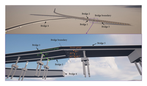
Bridge 1 is a prestressed concrete continuous curved box girder bridge, with four spans in total, each consisting of three spans. The span combinations are as follows: (3 × 30) m + (3 × 30) m + (30 + 2 × 35) m + (35 + 43 + 28) m. The box girder has a single-box single-cell cross section with a total width of 9.5 m. The third span is located on a horizontal curve with a radius of 103.75 m.

Bridge 2 is a north–south straight bridge with a total length of 274.8 m. The superstructure is a prestressed concrete continuous box girder with span combinations of (3 × 27) m + (2 × 27 + 23.5) m + (30 + 32 + 26.3 + 28) m. The box girder has a single-box single-cell cross section with a total width of 10.5 m.

Bridge 5 connects Bridge 1 and Bridge 2 with a single-span curved girder segment, with a total length of 56 m. The superstructure consists of 2 × 28 m of prestressed concrete continuous box girders, with a single-box three-cell cross section. Rubber expansion joints are installed at the abutments and segment connections. The transition pier cap beams are designed as hidden cap beams, and the transition pier bearings use rectangular plate rubber bearings.

Due to the single-column pier single-support design of Bridges 1 and 2, along with the relatively narrow bridge deck, it is essential to focus on the anti-overturning stability under eccentric loading conditions. Therefore, displacement gauges are installed on both sides of the girder bottoms of these two bridges to monitor the rotational status and assess the overturning risk. Bridge 5, with a large box-section girder, supports four lanes of traffic. With the city’s development, overloading incidents occur from time to time. Consequently, strain sensors have been installed at the bottom of the girder to monitor the bearing performance.

This study selected eight sensors from the group of bridges for spatiotemporal correlation modeling: two displacement gauges on both sides of the girder bottom of Bridge 1, two displacement gauges on both sides of the girder bottom of Bridge 2, and four strain gauges at the midspan of the girder bottom of Bridge 5. The sensors on the three bridges are all located on neighboring spans, and the load fields, such as traffic flow and temperature, are interconnected. The strain on Bridge 5 and the displacements on Bridges 1 and 2 exhibit spatiotemporal correlations. The proposed model in the study is designed to be flexible and can be extended to various types of monitoring data, beyond just bridge tilt and displacement prediction.

Optimizing sensor placement is essential not only for modeling spatial correlations but also for monitoring multiple structural behaviors. In this study, longitudinal sensor spacing is determined based on the specific monitoring tasks of different sensor types. Strain gauges are positioned to capture the bending performance of the monitored span, while displacement gauges are placed atop piers to track bearing displacements. If the sole focus is on spatial correlation, the average speed of vehicles on the monitored lane is considered to optimize sensor spacing for timely tilt warnings.

4.2. Measured Critical Responses

The critical response data collected from the SHM systems of three bridges are gathered over a period of time. These raw data are preprocessed to enhance the data quality. The locally weighted scatterplot smoothing (LOWESS) technique is used to reduce sensor noise while preserving essential structural response characteristics. Outliers are identified using z-score analysis and subsequently reviewed for potential data errors. Outlier data points of one sensor are removed for all sensors at the same time. No missing data occurred. Following preprocessing, the refined data are consolidated into a structured database for subsequent spatial analysis. This database forms the basis for further modeling of spatiotemporal correlations.

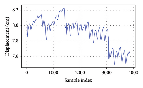
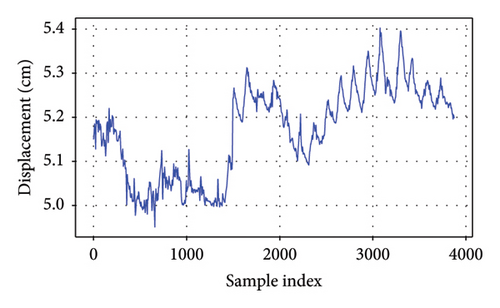
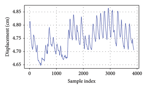
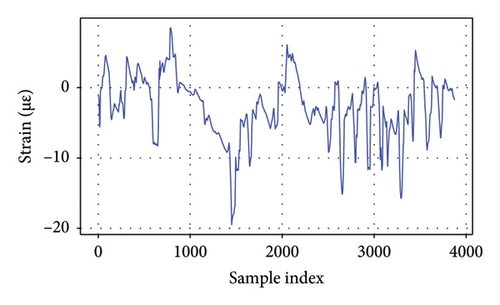
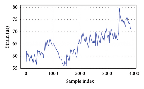
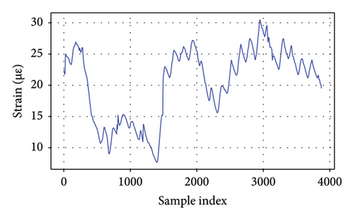
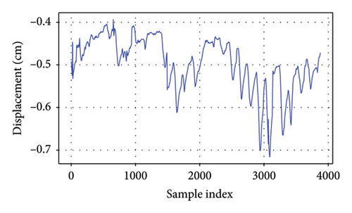
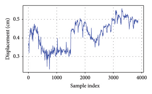
The eight responses are labeled as follows: left displacement gauge of girder bottom of Bridge 1 (B1^L), right displacement gauge of girder bottom of Bridge 1 (B1^R), left displacement gauge of girder bottom of Bridge 2 (B2^L), right displacement gauge of girder bottom of Bridge 2 (B2^R), left side strain gauge of girder bottom of Bridge 5 (B5^LL), middle left strain gauge of girder bottom of Bridge 5 (B5^ML), middle right strain gauge of girder bottom of Bridge 5 (B5^MR), and middle right strain gauge of girder bottom of Bridge 5 (B5^RR).

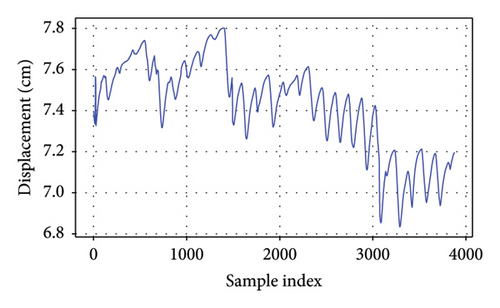
As depicted in Figure 4, it is evident that these responses display distinctive characteristics for each bridge. The girder displacement of B1^L and B1^R fluctuates within a range of 1 cm, whereas the girder displacement of B2^L and B2^R varies within a narrower range of 0.5 cm. These differences likely stem from variations in structural stiffness and applied loads. The strain measured by the strain gauges on Bridge 5 falls within a range of 30 με for each gauge. These fluctuations underscore the dynamic nature of structural performance and emphasize the significance of accounting for seasonal variations when evaluating bridge behavior and integrity. The EL framework can capture long-term variations in bridge behavior by learning patterns across different time periods. GPR as the meta-model could incorporate uncertainty estimation, allowing the model to adapt to seasonal shifts.

4.3. Copula-Based Probabilistic Modeling

The copula-based probabilistic modeling primarily serves to reveal the dependence structure between critical structural responses of neighboring bridges. The overturning performance of Bridge 1 and Bridge 2 is directly related to the difference in displacement measurements on their respective bottom sides. For Bridge 5, as the locations of the strain sensors are close to the displacement meters of Bridge 1 and Bridge 2, it is assumed that vehicles do not transverse such a short distance between the ramps. Therefore, the difference between the two strain sensors on Bridge 5, corresponding to the respective displacement gauges of Bridge 1 and Bridge 2, is also calculated to represent the difference in vehicle loads on the sides of the ramps, which is directly relevant to overturning.

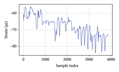
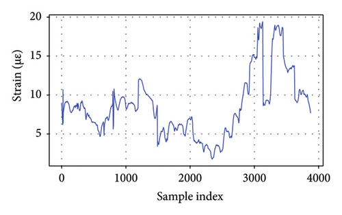
Furthermore, the four difference responses are labeled as follows: lateral tilt displacement of Bridge 1 (B1_diff), lateral tilt displacement of Bridge 2 (B2_diff), strain difference of the left side of Bridge 5 (), and strain difference of the right side of Bridge 5 (). Since the plotted responses in Figure 5 are directly derived from the original response differences, they also exhibit similar features to those in Figure 4 for each bridge.

The inherent correlations of structural responses of neighboring bridges could be initially revealed from the probabilistic perspectives. The copula theory provides a powerful tool for determining dependence among a set of variables. In particular, Gaussian copulas are particularly useful for capturing nonlinear relationships among variables with the Gaussian mixture distribution model as marginal distributions. While the individual Gaussian components in the marginal distributions assume a linear relationship, their combination can approximate nonlinear relationships. This allows for flexible parameter adjustments to effectively model data behavior, and the approach can be extended to more sophisticated models.

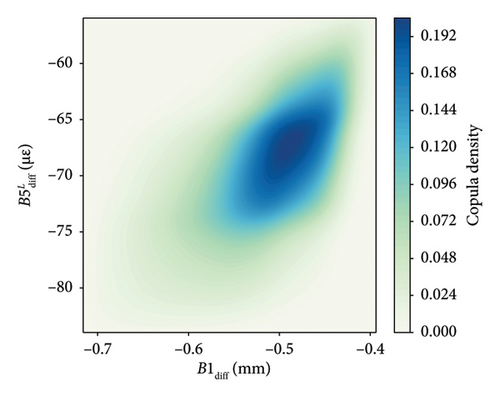
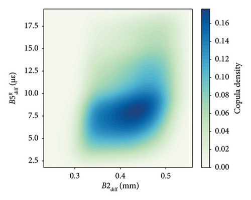
Figure 6 illustrates the copula-based joint density for critical responses of neighboring bridges. To explore the spatial correlation between neighboring spans, pairs are constructed between B1_diff and , as well as between B2_diff and . These visualizations offer valuable insights into the interdependencies between different response variables over time. The correlation between B1_diff and appears more concentrated than that between B2_diff and , indicating that the behavior of responses between B2_diff and involves more uncertainties. The overloading on the left side of Bridge 5 may visibly contribute to the significant tilt of Bridge 1. This observation aligns with the larger range of B1_diff compared to B2_diff in Figure 5. The copula analysis quantifies the joint dependence structure among response variables, offering insights into their probabilistic correlations. As for temporal correlation, the SHM system continuously collects response data over time, allowing the model to learn temporal patterns in displacement and tilt behavior. The meta-model within the ensemble framework could account for time-dependent variations by incorporating sequential training and uncertainty quantification.

5. AL-Enhanced EL Spatiotemporal Modeling

5.1. Modeling

In the model tuning, Bayesian optimization is used to optimize the hyperparameters of the proposed ensemble model. Bayesian optimization not only identifies the optimal settings for key parameters, such as the learning rate and number of trees for the gradient boosting and random forest regressors, as well as the kernel parameters for the Gaussian process regression, but also provides insight into the sensitivity of the model’s performance to these hyperparameters. By systematically exploring the hyperparameter space, Bayesian optimization reveals the impact of parameter variations on prediction accuracy and overall model stability.

The AL-enhanced EL model for predicting the vertical displacement of Bridge 1 and Bridge 2 from measured strains of neighboring Bridge 5 is trained and tested with the split dataset with the ratio of 7 : 3. Figure 7 shows the prediction results with the confidence intervals in the untrained test dataset for four target displacements on Bridge 1 and Bridge 2. Since the test dataset contains thousands of samples, Figure 7 only shows 200 samples for a clear illustration. Any discrepancies between the predicted and actual values are minimal and fall within the confidence intervals, suggesting that the model effectively captures the underlying behavior of bridge performance.

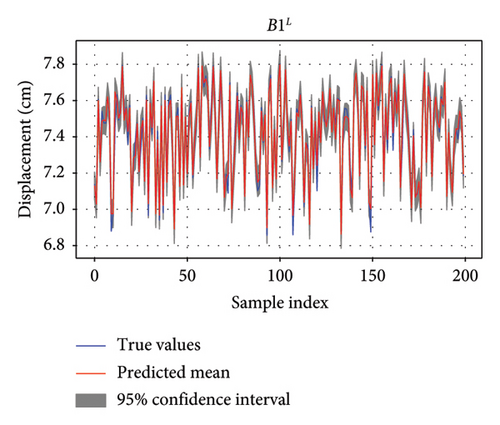
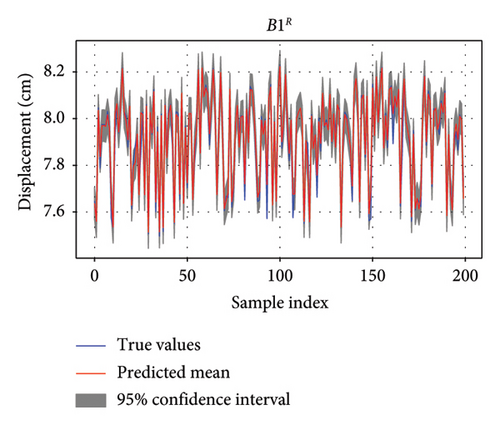
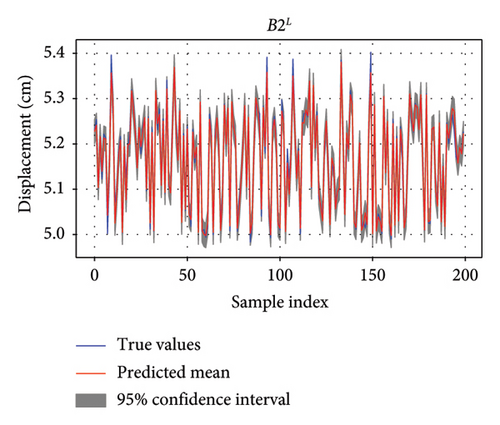
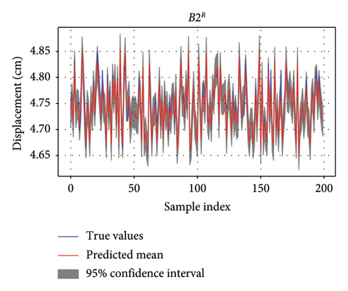
It could be seen that the prediction mean and ground truth match well in time series. The confidence intervals around the predictions provide a measure of the uncertainty, with narrower intervals suggesting higher confidence in the predictions. In Figure 7, the gray shading represents uncertainty or confidence interval. The confidence intervals for B1^L, B1^R, and B2^L are narrower than that for B2^R, reflecting more precise predictions for Bridge 1 and vertical displacement of Bridge 2 in the left side. The confidence intervals are slightly wider, reflecting greater uncertainty, but the predictions are still within an acceptable range.

The predictions are then compared to the ground truth data to evaluate the model’s performance using all test data in the scatter plot. Coefficient determination is used as the metric to evaluate performance. The results, depicted in Figure 8, show that the predicted vertical displacements for B1^L, B1^R, and B2^L exhibit a higher degree of correlation compared to B2^R. These three predictions have coefficient of determinations (R²) [46] over 95%, largest R² value is 98.29% for the prediction of B2^L. When only using one of the three stacked regressors, the R² value is lower than the stacked EL regressors.

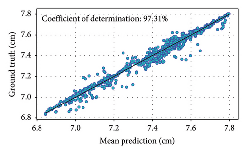
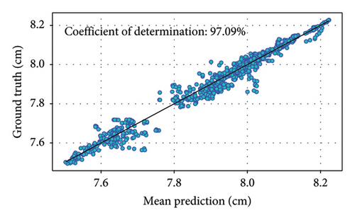
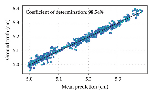
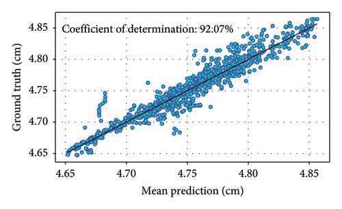
These predicted vertical displacements closely follow the ground truth data, with minor deviations. This indicates that the vertical displacement of B1^L, B1^R, and B2^L is more sensitive to the loads on Bridge 5, likely due to their structural proximity and interdependencies. The close alignment between predicted and ground truth data for both bridges demonstrates the reliability of the AL-enhanced EL method. The trained EL model also successfully models the spatiotemporal correlation of responses of neighboring bridges.

5.2. AL Enhancement in Model Performance

AL is used to iteratively refine the model by selecting the most uncertain samples for labeling and retraining. Specifically, the entropy-based approach quantifies the uncertainty of each prediction. At each iteration, samples with the highest predictive uncertainty are selected for labeling, ensuring that the most informative data points are incorporated into the training process. The tuning strategy helps balance the exploration of high-uncertainty regions with the exploitation of areas where the model already performs well. This adaptive approach maintains high accuracy and efficiency even as data characteristics evolve over time.

This study trains the model with sample ratios ranging from 0.1 to 0.8 of the entire training datasets. Figure 9(a) shows the effect of the initial training data on model performance, measured by R². The results indicate that increasing the sampling ratio improves the model’s accuracy, with a higher sample ratio leading to better prediction accuracy.

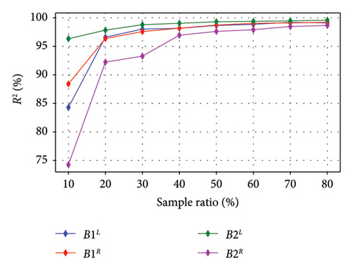
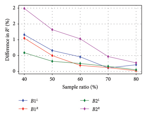
However, AL does not necessarily enhance the model’s accuracy or efficiency directly. Instead, the accuracy improves with a higher sampling ratio, while a lower sampling ratio helps reduce training time, thus improving efficiency. The model trained without AL, using the entire dataset, achieves an R² value of around 99% for each response. Figure 9(b) shows that when the AL-enhanced model uses only 40% of the dataset, the accuracy difference between it and the baseline model is less than 2%. This suggests that a smaller sample ratio can still maintain high accuracy while reducing training time.

The training dataset is selected based on an AL strategy, which prioritizes the most informative samples to improve model efficiency and accuracy. This approach mitigates the risk of introducing bias due to arbitrary sample selection. Additionally, the selected dataset comprises real-world SHM measurements collected over an extended period, minimizing selection bias that could arise from short-term or artificially controlled experiments.

5.3. Tilt Predictions

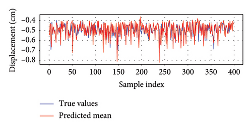
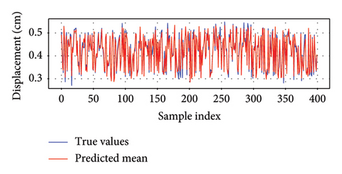
The tilt predictions for Bridge 1 and Bridge 2 are calculated based on the prediction means from the trained model, using the differences between B1^L and B1^R, as well as between B2^L and B2^R, as illustrated in Section 4.3. The trained model leverages the AL-enhanced EL approach, which ensures that the most informative samples are utilized to improve prediction accuracy effectively.

Figure 10 shows the comparison of tilt predictions with the ground truth measurements for the two bridges. The predicted tilt values align closely with the ground truth data for both Bridge 1 and Bridge 2. It captures the dynamic behavior of the bridge tilts, reflecting the structural responses accurately over time. The successful prediction of bridge tilt behavior indicates that the model can be used as a predictive tool for monitoring the structural health of bridges. Specifically, the model has potential applications in real-time overturning warnings, providing early alerts based on predicted tilt values.

The use of AL in this study, despite the availability of real-time sensor data, is justified by several key factors: (1) Efficient data utilization: Although the data are collected in real time, not all data points contribute equally to the model’s learning process. AL helps identify and prioritize the most informative samples that can significantly improve the model’s performance. This selective approach ensures that the model focuses on the most relevant data, reducing the time and computational resources needed for training. (2) Adapting to changing conditions: Bridge responses can vary due to factors like environmental changes, traffic patterns, and structural aging. AL enables the model to adapt to these changes by continually selecting the most informative new data, ensuring that the model remains accurate and relevant over time.

6. Conclusions

This study demonstrates that an AL-enhanced EL model can accurately and efficiently predict the tilt behavior of adjacent bridges. Critical response data from three neighboring bridges are gathered using SHM systems. An EL model is developed, incorporating gradient boosting, random forest, and Gaussian process regressors to output means and standard deviation of predictions. AL is also added to iteratively selecting the most informative samples, thereby enhancing the model’s accuracy and efficiency. In the case study, the model can precisely predict the displacement of Bridge 1 and Bridge 2 using strain data from Bridge 5. Copula theory is applied to model the dependence structure between different response variables, providing insights into their interdependence. The spatial and temporal correlations between the responses of the neighboring bridges are determined. Key conclusions are as follows:

1.
The model demonstrates high accuracy in predicting the vertical displacement and tilt of Bridge 1 and Bridge 2. The close match between the predicted and actual values indicates that the trained model effectively captures the dynamic behavior of the bridges and extracts spatial and temporal correlations among neighboring bridges. This performance is a result of the combined strengths of the EL approach and the AL strategy.
2.
By employing AL, this study shows that the model’s performance improves significantly, especially in the early stages of training, making the model both more accurate and efficient. The comparison with the baseline model underscores the effectiveness of AL in enhancing model accuracy with only 40% of samples.
3.
The spatial and temporal correlations between the responses of the neighboring bridges are well represented in the model. The strong correlation between B1_diff and versus the weaker correlation between B2_diff and suggests different structural interdependencies, reflecting varying levels of stiffness and load distribution.
4.
The successful prediction of bridge tilt behavior shows that the model can be used for real-time SHM. It has the potential to provide early warnings for possible overturning, allowing for timely interventions and enhancing bridge safety.

The methodology can be expanded to incorporate more complex models and additional data sources, including environmental factors, traffic load variations, and datasets from various geographical locations and bridge configurations. Incorporating temperature, wind speed, and traffic loads will provide a more comprehensive understanding of how these variables impact bridge behavior. Further refinement of AL techniques will continue to improve model adaptability.

Disclosure

The conclusions and opinions in this paper are of the authors, which do not necessarily reflect that of the bridge operator or the inspection company.

Conflicts of Interest

The authors declare no conflicts of interest.

Author Contributions

Ru An: software, data curation, investigation, and project administration. Mengjin Sun: formal analysis, methodology, and writing – original draft. You Dong: writing – review and Editing and supervision. Lu Guo: resources and software. Lei Jia: validation, writing – review and editing, visualization, and funding acquisition. Xiaoming Lei: conceptualization, methodology, software, writing – original draft, and visualization. Ru An and Mengjin Sun, the first two authors, contributed equally to this work.

Funding

The authors would like to acknowledge financial support from the National Key R&D Program of China (2022YFC3801100 and 2022YFC3801102), Shenzhen Science and Technology Program (KJZD20240903102742055), Natural Science Foundation of Shanghai (24ZR1460700), Shanghai Research Institute of Building Sciences Co. Ltd. (KY10000038.20230043), and the Hong Kong Polytechnic University (P0054456).

Acknowledgments

Open Research

Data Availability Statement

All data included in this study are available from the corresponding author upon request.

References

1 Xiong W., Cai C. S., Kong B., and Ye J. S., Overturning-Collapse Modeling and Safety Assessment for Bridges Supported by Single-Column Piers, Journal of Bridge Engineering. (2017) 22, no. 11, https://doi.org/10.1061/(asce)be.1943-5592.0001133, 2-s2.0-85027838640.
10.1061/(ASCE)BE.1943-5592.0001133
Web of Science® Google Scholar
2 Xu F. Y., Zhang M. J., Wang L., and Zhang J. R., Recent Highway Bridge Collapses in China: Review and Discussion, Journal of Performance of Constructed Facilities. (2016) 30, no. 5, https://doi.org/10.1061/(asce)cf.1943-5509.0000884, 2-s2.0-84988375045.
10.1061/(ASCE)CF.1943-5509.0000884
Web of Science® Google Scholar
3 Lei X. M., Dong Y., and Frangopol D. M., Sustainable Life-Cycle Maintenance Policymaking for Network-Level Deteriorating Bridges With a Convolutional Autoencoder-Structured Reinforcement Learning Agent, Journal of Bridge Engineering. (2023) 28, no. 9, https://doi.org/10.1061/jbenf2.beeng-6159.
10.1061/JBENF2.BEENG-6159
Web of Science® Google Scholar
4 Yang D. H., Guan Z. X., Yi T. H., Li H. N., and Ni Y. S., Fatigue Evaluation of Bridges Based on Strain Influence Line Loaded by Elaborate Stochastic Traffic Flow, Journal of Bridge Engineering. (2022) 27, no. 9, https://doi.org/10.1061/(asce)be.1943-5592.0001929.
10.1061/(ASCE)BE.1943-5592.0001929
Web of Science® Google Scholar
5 Niu J., Li Z. L., Zhuo Y. et al., Robust Correlation Mapping of Train-Induced Stresses for High-Speed Railway Bridge Using Convolutional Denoising Autoencoder, Structural Health Monitoring. (2023) 22, no. 2, 832–845, https://doi.org/10.1177/14759217221095191.
10.1177/14759217221095191
Web of Science® Google Scholar
6 Jiang F., Ding Y. L., Song Y. S., Geng F. F., and Wang Z. W., Digital Twin-Driven Framework for Fatigue Lifecycle Management of Steel Bridges, Structure and Infrastructure Engineering. (2023) 19, no. 12, 1826–1846, https://doi.org/10.1080/15732479.2022.2058563.
10.1080/15732479.2022.2058563
Web of Science® Google Scholar
7 Zhang Y. M., Wang H., Bai Y., Mao J. X., Chang X. Y., and Wang L. B., Switching Bayesian Dynamic Linear Model for Condition Assessment of Bridge Expansion Joints Using Structural Health Monitoring Data, Mechanical Systems and Signal Processing. (2021) 160, https://doi.org/10.1016/j.ymssp.2021.107879.
10.1016/j.ymssp.2021.107879
Web of Science® Google Scholar
8 Zhang X. N., Ding Y. L., Zhao H. W., and Yi L. T., Long-Term Bridge Performance Assessment Using Clustering and Bayesian Linear Regression for Vehicle Load and Strain Mapping Model, Structural Control and Health Monitoring. (2022) 29, no. 12, https://doi.org/10.1002/stc.3118.
10.1002/stc.3118
PubMed Web of Science® Google Scholar
9 Lei X., Dong Y., and Frangopol D., Integration of Inspection and Monitoring Data for RL-Enhanced Sustainable Life-Cycle Management of Infrastructure Networks, Structure and Infrastructure Engineering. (2025) 1–15, https://doi.org/10.1080/15732479.2025.2453484.
10.1080/15732479.2025.2453484
Web of Science® Google Scholar
10 Cao J. X. and Liu Y., Damage Localization for Bridges Monitored Within One Cluster Based on a Spatiotemporal Correlation Model of Strain Monitoring Data, Structural Health Monitoring. (2023) 22, no. 1, 105–130, https://doi.org/10.1177/14759217221078766.
10.1177/14759217221078766
Web of Science® Google Scholar
11 Cao J. X., Zhang S. Y., and Liu Y., Probabilistic SDDLV Method for Localizing Damage in Bridges Monitored Within One Cluster Under Time-Varying Environmental Temperatures, Journal of Civil Structural Health Monitoring. (2022) 12, no. 1, 47–70, https://doi.org/10.1007/s13349-021-00524-6.
10.1007/s13349-021-00524-6
Web of Science® Google Scholar
12 Cao J. X., Zhou Z., and Liu Y., Damage Localization for Prefabricated Bridges Group Using the Area-Ratio of the Strain Time-History Curve, Measurement. (2022) 198, https://doi.org/10.1016/j.measurement.2022.111172.
10.1016/j.measurement.2022.111172
Web of Science® Google Scholar
13 Peng W. B., Zhao H., Dai F., and Taciroglu E., Analytical Method for Overturning Limit Analysis of Single-Column Pier Bridges, Journal of Performance of Constructed Facilities. (2017) 31, no. 4, https://doi.org/10.1061/(asce)cf.1943-5509.0000999, 2-s2.0-85018374390.
10.1061/(ASCE)CF.1943-5509.0000999
Web of Science® Google Scholar
14 Qin L. F., Ren W. X., and Guo C. R., A Physics-Data Hybrid Framework to Develop Bridge Digital Twin Model in Structural Health Monitoring, International Journal of Structural Stability and Dynamics. (2023) 23, no. 16n18, https://doi.org/10.1142/s0219455423400370.
10.1142/S0219455423400370
Web of Science® Google Scholar
15 Shi X. F., Zhou Z. J., and Ruan X., Failure Analysis of a Girder Bridge Collapse Under Eccentric Heavy Vehicles, Journal of Bridge Engineering. (2016) 21, no. 12, https://doi.org/10.1061/(asce)be.1943-5592.0000964, 2-s2.0-84995750506.
10.1061/(ASCE)BE.1943-5592.0000964
Web of Science® Google Scholar
16 Shi X. F., Cao Z., Ma H. Y., and Ruan X., Failure Analysis on a Curved Girder Bridge Collapse Under Eccentric Heavy Vehicles Using Explicit Finite Element Method: Case Study, Journal of Bridge Engineering. (2018) 23, no. 3, https://doi.org/10.1061/(asce)be.1943-5592.0001201, 2-s2.0-85040635961.
10.1061/(ASCE)BE.1943-5592.0001201
Web of Science® Google Scholar
17 Guo H., Dong Y., Bastidas-Arteaga E., and Lei X., Life-Cycle Performance Prediction and Interpretation for Coastal and Marine RC Structures: An Ensemble Learning Framework, Structural Safety. (2024) 110, https://doi.org/10.1016/j.strusafe.2024.102496.
10.1016/j.strusafe.2024.102496
Web of Science® Google Scholar
18 Li J. and Hao H., Damage Detection of Shear Connectors Under Moving Loads With Relative Displacement Measurements, Mechanical Systems and Signal Processing. (2015) 60-61, 124–150, https://doi.org/10.1016/j.ymssp.2014.09.014, 2-s2.0-84925937733.
10.1016/j.ymssp.2014.09.014
Web of Science® Google Scholar
19 Zhang W., Sun L. M., and Sun S. W., Bridge-Deflection Estimation Through Inclinometer Data Considering Structural Damages, Journal of Bridge Engineering. (2017) 22, no. 2, https://doi.org/10.1061/(asce)be.1943-5592.0000979, 2-s2.0-85009811749.
10.1061/(ASCE)BE.1943-5592.0000979
Web of Science® Google Scholar
20 Ge L. F., Dan D. H., Yan X. F., and Zhang K. L., Real Time Monitoring and Evaluation of Overturning Risk of Single-Column-Pier Box-Girder Bridges Based on Identification of Spatial Distribution of Moving Loads, Engineering Structures. (2020) 210, https://doi.org/10.1016/j.engstruct.2020.110383.
10.1016/j.engstruct.2020.110383
Web of Science® Google Scholar
21 Dan D. H., Yu X. W., Yan X. F., and Zhang K. L., Monitoring and Evaluation of Overturning Resistance of Box Girder Bridges Based on Time-Varying Reliability Analysis, Journal of Performance of Constructed Facilities. (2020) 34, no. 1, https://doi.org/10.1061/(asce)cf.1943-5509.0001375.
10.1061/(ASCE)CF.1943-5509.0001375
Web of Science® Google Scholar
22 Ye X. W., Sun Z., and Lu J., Prediction and Early Warning of Wind-Induced Girder and Tower Vibration in Cable-Stayed Bridges With Machine Learning-Based Approach, Engineering Structures. (2023) 275, https://doi.org/10.1016/j.engstruct.2022.115261.
10.1016/j.engstruct.2022.115261
Web of Science® Google Scholar
23 Chang S. J. and Kim N. S., Development of Smart Seismic Bridge Bearing Using Fiber Optic Bragg-Grating Sensors, Proceedings of the Conference on Sensors and Smart Structures Technologies for Civil, Mechanical, and Aerospace Systems, 2013, San Diego.
Google Scholar
24 Xu Q. E., Gao Q. F., and Liu Y., A Method for Suspenders Tension Identification of Bridges Based on the Spatio-Temporal Correlation Between the Girder Strain and Suspenders Tension, Computer-Aided Civil and Infrastructure Engineering. (2024) 39, no. 11, 1641–1658, https://doi.org/10.1111/mice.13165.
10.1111/mice.13165
Web of Science® Google Scholar
25 Lei X. M., Xia Y., Komarizadehasl S., and Sun L. M., Condition Level Deteriorations Modeling of RC Beam Bridges With U-Net Convolutional Neural Networks, Structures. (2022) 42, 333–342, https://doi.org/10.1016/j.istruc.2022.06.013.
10.1016/j.istruc.2022.06.013
Web of Science® Google Scholar
26 Liu H. and Zhang Y. F., Bridge Condition Rating Data Modeling Using Deep Learning Algorithm, Structure and Infrastructure Engineering. (2020) 16, no. 10, 1447–1460, https://doi.org/10.1080/15732479.2020.1712610.
10.1080/15732479.2020.1712610
Web of Science® Google Scholar
27 Lai L., Dong Y., Andriotis C. P., Wang A. J., and Lei X. M., Synergetic-Informed Deep Reinforcement Learning for Sustainable Management of Transportation Networks With Large Action Spaces, Automation in Construction. (2024) 160, https://doi.org/10.1016/j.autcon.2024.105302.
10.1016/j.autcon.2024.105302
Web of Science® Google Scholar
28 Lei X. M., Xia Y., Wang A., Jian X. D., Zhong H. Q., and Sun L. M., Mutual Information Based Anomaly Detection of Monitoring Data With Attention Mechanism and Residual Learning, Mechanical Systems and Signal Processing. (2023) 182, https://doi.org/10.1016/j.ymssp.2022.109607.
10.1016/j.ymssp.2022.109607
Web of Science® Google Scholar
29 Lei X. M., Sun L. M., and Xia Y., Lost Data Reconstruction for Structural Health Monitoring Using Deep Convolutional Generative Adversarial Networks, Structural Health Monitoring. (2021) 20, no. 4, 2069–2087, https://doi.org/10.1177/1475921720959226.
10.1177/1475921720959226
Web of Science® Google Scholar
30 Sarmadi H., Entezami A., and Magalhaes F., Unsupervised Data Normalization for Continuous Dynamic Monitoring by an Innovative Hybrid Feature Weighting-Selection Algorithm and Natural Nearest Neighbor Searching, Structural Health Monitoring. (2023) 22, no. 6, 4005–4026, https://doi.org/10.1177/14759217231166116.
10.1177/14759217231166116
Web of Science® Google Scholar
31 Feng D. C., Wang W. J., Mangalathu S., and Sun Z., Condition Assessment of Highway Bridges Using Textual Data and Natural Language Processing-(NLP-) Based Machine Learning Models, Structural Control and Health Monitoring. (2023) 2023, 1–17, https://doi.org/10.1155/2023/9761154.
10.1155/2023/9761154
Web of Science® Google Scholar
32 Lei X. M., Sun M. J., Zhao R. X. et al., Unsupervised Vision-Based Structural Anomaly Detection and Localization With Reverse Knowledge Distillation, Structural Control and Health Monitoring. (2024) 2024, no. 1, https://doi.org/10.1155/2024/8933148.
10.1155/2024/8933148
Web of Science® Google Scholar
33 Lei X. M., Siringoringo D. M., Dong Y., and Sun Z., Interpretable Machine Learning Methods for Clarification of Load-Displacement Effects on Cable-Stayed Bridge, Measurement. (2023) 220, https://doi.org/10.1016/j.measurement.2023.113390.
10.1016/j.measurement.2023.113390
Web of Science® Google Scholar
34 Han Q. H., Ma Q., Dang D. Z., and Xu J., Modal Parameters Prediction and Damage Detection of Space Grid Structure Under Environmental Effects Using Stacked Ensemble Learning, Structural Control and Health Monitoring. (2023) 2023, 1–24, https://doi.org/10.1155/2023/5687265.
10.1155/2023/5687265
Web of Science® Google Scholar
35 Sun Z., Ye X. W., and Lu J., Estimating Stay Cable Vibration Under Typhoon With an Explainable Ensemble Learning Model, Structure and Infrastructure Engineering. (2023) 20, no. 12, 1912–1924, https://doi.org/10.1080/15732479.2023.2165121.
10.1080/15732479.2023.2165121
Web of Science® Google Scholar
36 Yaghoubzadehfard A., Lumantarna E., Herath N., Sofi M., and Rad M., Ensemble Learning-Based Structural Health Monitoring of a Bridge Using an Interferometric Radar System, Journal of Civil Structural Health Monitoring. (2024) 14, no. 7, 1629–1650, https://doi.org/10.1007/s13349-024-00789-7.
10.1007/s13349-024-00789-7
Web of Science® Google Scholar
37 Moustapha M., Marelli S., and Sudret B., Active Learning for Structural Reliability: Survey, General Framework and Benchmark, Structural Safety. (2022) 96, https://doi.org/10.1016/j.strusafe.2021.102174.
10.1016/j.strusafe.2021.102174
Web of Science® Google Scholar
38 Lei X., Sun Z., Wang A., Guo T., and Nagayama T., Estimation of Bridge Girder Cumulative Displacement for Component Operational Warning Using Bayesian Neural Networks, Structural Control and Health Monitoring. (2025) 2025, no. 1, https://doi.org/10.1155/stc/9974584.
10.1155/stc/9974584
Web of Science® Google Scholar
39 Dang C., Valdebenito M. A., Faes M. G. R., Song J. W., Wei P. F., and Beer M., Structural Reliability Analysis by Line Sampling: A Bayesian Active Learning Treatment, Structural Safety. (2023) 104, https://doi.org/10.1016/j.strusafe.2023.102351.
10.1016/j.strusafe.2023.102351
Web of Science® Google Scholar
40 Zhou T., Guo T., Dong Y., Yang F., and Frangopol D. M., Look-Ahead Active Learning Reliability Analysis Based on Stepwise Margin Reduction, Reliability Engineering & System Safety. (2024) 243, https://doi.org/10.1016/j.ress.2023.109830.
10.1016/j.ress.2023.109830
Web of Science® Google Scholar
41 Bull L. A., Gardner P., Rogers T. J., Cross E. J., Dervilis N., and Worden K., Probabilistic Inference for Structural Health Monitoring: New Modes of Learning From Data, ASCE-ASME Journal of Risk and Uncertainty in Engineering Systems Part A-Civil Engineering. (2021) 7, no. 1, https://doi.org/10.1061/ajrua6.0001106.
10.1061/ajrua6.0001106
Web of Science® Google Scholar
42 Bull L., Worden K., Manson G., and Dervilis N., Active Learning for Semi-Supervised Structural Health Monitoring, Journal of Sound and Vibration. (2018) 437, 373–388, https://doi.org/10.1016/j.jsv.2018.08.040, 2-s2.0-85053833137.
10.1016/j.jsv.2018.08.040
Web of Science® Google Scholar
43 Bull L. A., Rogers T. J., Wickramarachchi C., Cross E. J., Worden K., and Dervilis N., Probabilistic Active Learning: An Online Framework for Structural Health Monitoring, Mechanical Systems and Signal Processing. (2019) 134, https://doi.org/10.1016/j.ymssp.2019.106294, 2-s2.0-85071600709.
10.1016/j.ymssp.2019.106294
Web of Science® Google Scholar
44 Hughes A. J., Bull L. A., Gardner P., Barthorpe R. J., Dervilis N., and Worden K., On Risk-Based Active Learning for Structural Health Monitoring, Mechanical Systems and Signal Processing. (2022) 167, https://doi.org/10.1016/j.ymssp.2021.108569.
10.1016/j.ymssp.2021.108569
Web of Science® Google Scholar
45 Zhu R., Chen Y., Peng W. W., and Ye Z. S., Bayesian Deep-Learning for RUL Prediction: An Active Learning Perspective, Reliability Engineering & System Safety. (2022) 228, https://doi.org/10.1016/j.ress.2022.108758.
10.1016/j.ress.2022.108758
Web of Science® Google Scholar
46 Rezazadeh N., Perfetto D., de Oliveira M., De Luca A., and Lamanna G., A Fine-Tuning Deep Learning Framework to Palliate Data Distribution Shift Effects in Rotary Machine Fault Detection, Structural Health Monitoring. (2024) https://doi.org/10.1177/14759217241295951.
10.1177/14759217241295951
Web of Science® Google Scholar

All articles

Active Learning–Enhanced Ensemble Method for Spatiotemporal Correlation Modeling of Neighboring Bridge Behaviors to Girder Overturning

Abstract

1. Introduction

2. General Framework of AL-Enhanced EL for Response Modeling