Non-probabilistic Structural Damage Identification With Uncertainties by Phase Space–Based CNN
Abstract
Considering the critical role of uncertainties in structural damage detection, primarily arising from measurement errors and finite element model discrepancies, a nonprobabilistic approach based on interval analysis is proposed. This nonprobabilistic approach integrates phase space matrices with convolutional neural networks (CNNs) for damage identification. The compatibility of the phase space matrix data format with CNN allows for high sensitivity in detecting damage. Unlike probabilistic methods, this approach does not rely on specific probability distributions but considers the upper and lower bounds of uncertainties, making it highly applicable to real-world applications. The proposed method employs the phase space matrix as the input for the CNN and the elemental stiffness parameter (ESP) as the output. When accounting for uncertainties, distinct networks are developed from the upper and lower bounds of the input phase space matrix. Both the undamaged state and the state under assessment are processed through these networks. The resulting outputs enable the computation of the possibility of damage existence (PoDE) and the damage measure index (DMI), which collectively provide a comprehensive assessment of the level and probability of damage. Validation using a numerical model and experimental data confirms the effectiveness of this method in accurately determining the location and level of damage while considering uncertainties.
1. Introduction
With the growth of public infrastructure and its extended service life, there is an essential need to continuously monitor and detect possible damage in civil engineering structures. Beyond extending their lifespan, maintaining the structural integrity of these structures is crucial for ensuring safety and reliability [1, 2]. One efficient way of structural damage diagnosis is focusing on the structural properties of structures, such as vibration characteristics or vibration responses. When structural damage occurs, there will be alterations in structural parameters. These changes provide the basic to identify structural damage by using vibration characteristics or responses.
Damage identification can be directly inferred from changes in the structural dynamic characteristics, such as frequencies [3], mode shapes [4, 5], damping ratio [6, 7], and transmissibility [8]. Natural frequencies of civil structures can be usually measured, but minor deviations in these natural frequencies can be overlooked, since natural frequencies are less sensitive to slight damage. While mode shapes are much more sensitive to structural damage compared to natural frequency, it is pivotal to note that only the lower vibration mode shapes are easily measured, especially using a limited number of sensors. Hence, application of mode shapes could be limited in practical applications of comprehensive structural health monitoring. Additionally, acquiring and analyzing higher-order mode shapes can be complex and labor-intensive, which might impact the efficacy and cost-effectiveness of structural health monitoring systems. Accurately deriving damping ratios from experimental data is also challenging, given their susceptibility to external factors such as temperature and moisture levels. Transmissibility-based methods suffer from frequency band and reference dependencies. The phase space–based damage identification method has been proposed as an innovative approach to address challenges in structural health monitoring. This method emphasizes a high sensitivity to structural damage and can also minimize the number of sensors required during deployment [9, 10]. Previous studies have evidenced that this phase space–based method holds significant potential for damage detection in practical applications [11, 12].
The identification results can also be obtained by employing the dynamic parameters or responses as inputs for cutting-edge computational techniques such as wavelet transform or frequency domain transformation [13, 14], support vector machine [15], metaheuristic algorithms [16, 17], and artificial neural networks [18]. With the rapid development of computer hardware, deep learning has been widely applied in the field of structural health monitoring, such as in missing measurement data recovery [19], reconstruction of structural response [20], and nonlinear modeling [21]. Among various deep learning techniques, convolutional neural network (CNN) has emerged as a notably promising computational methodology in recent years. CNN, a specialized type of artificial neural network, is highly suited for the field of structural damage identification due to its significant advantages of feature learning capability, spatial invariance, efficient handling of large datasets, and robustness against noisy data [22, 23]. Many studies have employed CNN for the purpose of structural damage identification. For example, Feng et al. [24] proposed a concrete crack detection method using CNN. Won et al. utilized 1-dimensional CNN to detect damage of a simply supported beam [25]. The phase space technique has already been combined with deep learning in structural health monitoring [12]. The CNN is particularly well-suited for this application since the phase space matrix generated during reconstruction can be used as input to CNN. Leveraging CNN alongside the high sensitivity of phase space techniques offers a promising approach for structural damage identification, effectively addressing modelling uncertainties and enhancing robustness against measurement noise.
Uncertainties can arise from different sources [26, 27], making the precise detection and quantification of structural damage challenging. Measurement or transmission noise represents a primary source of uncertainties, arising from errors or limitations in sensing equipment and the data acquisition process [28, 29]. Additionally, when a damage detection method is based on data generated by a finite element model, modeling uncertainty emerges as another significant source of uncertainty. The finite element model may differ from real structure due to simplification of real structure, nonideal boundary conditions, inaccuracies of physical parameters, and nonlinear structural material properties. Consequently, modeling uncertainty can result in the finite element model failing to accurately represent the behavior of the real structure. If a damage identification method is heavily dependent on data generated from the finite element model, modeling uncertainty may affect the performance or accuracy of the damage identification method. Probabilistic methods have demonstrated their efficacy in managing noisy data and modeling uncertainties [30–32]. However, a key assumption underlying these methods is that the uncertain parameters adhere to a specific probability distribution [33]. This deterministic property on probability distribution may not always capture the complex, dynamic nature of real-world uncertainties, potentially limiting the accuracy or applicability of such methods in engineering scenarios. Furthermore, obtaining an accurate probability distribution often requires a vast amount of empirical data, which exacerbates the challenges of uncertainty analysis based on probabilistic methods.
Employing nonprobabilistic methods to analyze the uncertainty effect can effectively address the aforementioned issue. Most nonprobabilistic methods are based on interval analysis. The main concept of these techniques is to employ interval analysis on the uncertain parameter, considering the upper and lower bounds of these parameters, and then an output interval is obtained. For example, after considering the uncertainties of structural frequencies with interval analysis, the interval bounds of stiffness can be obtained, and the damage level can be assessed using the central value derived from the stiffness interval bounds [34]. To quantitatively assess the probability of structural damage, the possibility of damage existence (PoDE) based on interval analysis was introduced [35]. A high PoDE value signifies a greater probability of damage. However, PoDE often tends to overestimate the probability of damage occurrence. As an improvement, the damage measure index (DMI) was proposed [36]. DMI integrates the stiffness reduction factor (SRF) and PoDE, providing a comprehensive reflection of the level of structural damage and its probability. Compared to the probabilistic method, the nonprobabilistic method does not require a specific probability distribution of uncertainties. The nonprobabilistic method only necessitates the upper and lower bounds of uncertain parameters, making it more readily applicable in practical engineering scenarios.
- 1.
A novel nonprobabilistic approach to structural damage identification is proposed, integrating phase space matrix reconstruction with CNNs to account for uncertainties. The phase space matrix is obtained and employed as the CNN input, with elemental stiffness parameter (ESP) employed as the CNN output. The combination of the phase space technique and CNN enables the proposed approach to achieve the high sensitivity and noise immunity of the phase space–based method, while also benefiting from the robustness of CNNs. The high sensitivity of phase space technique allows for using minimal sensors to identify damage.
- 2.
The proposed approach applies interval analysis to process uncertainties, eliminating the need for specific probabilistic distributions and improving the robustness of damage identification under noisy and uncertain conditions. When considering uncertainties, the input phase space matrix is processed to derive the upper and lower bounds, which are separately input into the CNN, resulting in two distinct networks. Data from both the undamaged and damaged states are fed into the two networks, producing four outputs.
- 3.
A framework is developed to compute the PoDE and DMI using CNN outputs, providing a comprehensive evaluation of damage probability and level. Based on these outputs, the PoDE is computed. To better indicate damage, the DMI is also calculated.
The effectiveness and performance of the proposed approach are validated using both numerical and experimental studies.
2. Methodology
This study presents a nonprobabilistic method to identify structural damage, by employing the phase space matrix as CNN input to consider uncertainties. Initially, the structural acceleration responses in the time domain are used by performing a reconstruction process to generate the phase space matrix. This matrix then serves as the input to the CNN structure, targeting ESP as the output. Using a nonprobabilistic method based on interval analysis, uncertainties are taken into account by processing the input phase space matrix to determine its upper and lower bounds. These bounds are subsequently fed into the CNN independently, resulting in the training of two separate networks. Data from both the undamaged state and the state under evaluation are fed into the two networks, producing four distinct outputs. Based on these four outputs, a rectangle can be plotted on a coordinate system. The proportion of the rectangle intersected by the failure plane allows for the determination of PoDE. Given that PoDE could sometimes overestimate the probability of damage, DMI is introduced for a more accurate representation of the identified damage.
2.1. Phase Space Matrix Reconstruction
For a l-dimensional dynamic system, characterizing this system typically requires l independent variables or parameters. Within the realm of structural health monitoring, this implies that monitoring complex structures necessitates the deployment of a vast array of sensors. The phase space reconstruction theory provides an effective solution to this challenge, with these l independent parameters denoting the coordinates of the phase space. According to Takens’ embedding theorem, it is possible to recreate a trajectory in the phase space that mirrors the original dynamical attractor using just a single state variable [37]. This theorem not only highlights the inherent interconnectedness of the system’s state variables but also provides a robust mechanism to analyze complex systems with a limited observability. The time-delay embedding stands out as a foremost technique among all the phase space reconstruction methods. The time-delay embedding method uses past data from one variable, spaced at regular time intervals, to recreate the multidimensional phase space. This assists in capturing and understanding the behavior of the dynamic system more effectively.

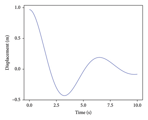
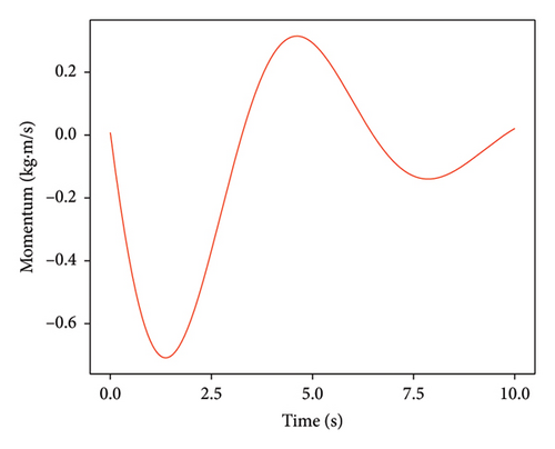
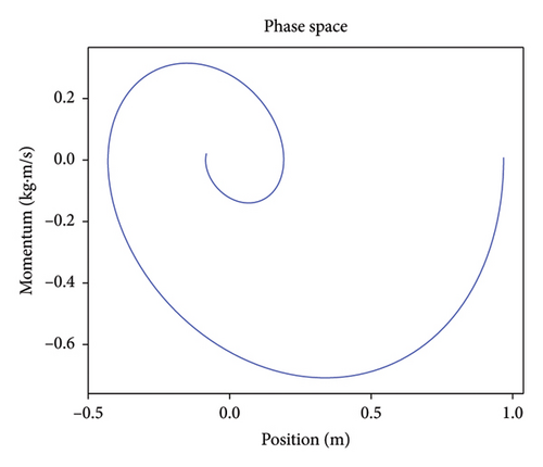
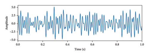
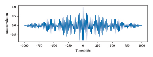
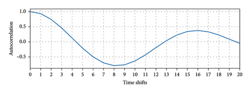
A method proposed by Krantz and Schreiber [39] can be used to calculate suitable values for t and m. As depicted in Figure 2, when performing cross-correlation analysis on the time-domain signal x, the autocorrelation sequence xc and the corresponding lag vector xlag can be obtained. By normalizing xc, a stacked line graph can be produced with xlag on the horizontal axis and xc on the vertical axis. By considering the region where xlag is larger than 0, the first point where the xc value reaches 0 is identified, and its corresponding lag value represents the delay time t. As depicted in Figure 2(c), the curve intersects the horizontal axis between coordinate values 4 and 5. Consequently, t is set to 5. Calculating the optimal dimension m is achieved through a process of trial and error experiment. An initially large value, labeled as mtry, is assumed. Using the delay time t that is previously identified, a phase space matrix is constructed. After the application of singular value decomposition (SVD) to this matrix, a diagonal matrix S is produced. The count of diagonal elements in S that significantly exceed 0 signifies the suitable value for m. With these suitable values of t and m, the dynamics of the system can be effectively represented in a phase space matrix.
2.2. CNN Model
As evidenced by prior studies [22, 40, 41], CNN has demonstrated its effectiveness in handling grid-like data and an exceptional accuracy in identifying structural damage [42, 43]. Since the phase space matrix is 2D grid data, which is particularly suited for CNN, in the proposed method, the input matrix consists of the phase space matrix, while the output corresponds to the damage levels of the structural elements. The architecture of the proposed CNN model consists of several layers, including input, convolutional, activation, pooling, fully connected, and output layers. The first layer receives the multidimensional phase space matrix, derived from the raw sensor data. In the following layers, feature extraction, pattern recognition, and damage level prediction are performed.
2.2.1. Convolutional Layer
The convolutional layer is designed for local feature extraction from the input matrix. The convolutional layer is the most crucial layer for extracting features from the input data; multiple filters (or kernels) are applied and convolved across the input matrix to produce feature maps. After feature maps are obtained, which serve as the input for the subsequent layer, all the weights in the kernels undergo gradient descent based on the backpropagation method, and then the optimal weights are obtained.
The proposed CNN model consists of multiple interconnected layers, each performing specific functions to process and analyze the input phase space matrix for structural damage identification. The convolutional layers extract local features by applying multiple filters to the input data, producing feature maps, with the kernel weights optimized using backpropagation. Batch normalization layers stabilize and accelerate training by normalizing intermediate activations and reducing internal covariate shifts. Nonlinearity is introduced through activation layers, typically using the rectified linear unit (ReLU), which enhances the training efficiency and addresses the gradient vanishing issue. Pooling layers compress the spatial dimensions of the feature maps via downsampling methods such as max pooling, ensuring that critical information is retained while improving noise robustness and computational efficiency. Fully connected layers integrate the extracted features to predict damage severities, linking the processed features to output neurons. Finally, the output layer transforms predictions into damage levels, providing an interpretable output that quantifies the structural health condition.
The proposed CNN model is trained using a collection of labeled phase space matrices. In this collection, the features of the input matrix are paired with the damage levels for every structural element. The aim during the training phase is to optimize the parameters of the model to reduce the loss function, typically the mean squared error (MSE) between the predicted damage levels and the actual ones. This training allows the model to establish mapping relationship between the features of the input matrix and the associated damage severities. The effectiveness of this learning can be measured using metrics, such as the R-squared (R2) value. To evaluate the generalization capability of the model across different datasets, it is trained on a designated training set, validated on a separate validation set, and tested on an independent testing subset. This rigorous evaluation process ensures that the model is not only effective under controlled conditions but also robust in varied real-world applications.
2.3. Residual Neural Network Model
In dealing with complex structures and multiple components, standard CNN often struggles to converge effectively. Residual convolutional neural network (ResNet) represents a class of deep CNNs that have gained significant interest because of its remarkable advantage over conventional plain CNNs. The unique feature of ResNet is its capability to address the vanishing gradient issue that is commonly observed in deep networks [31].
In standard CNNs, as the depth of the network expands, gradients can diminish or vanish during backpropagation, limiting ability to learn and hindering convergence. ResNet addresses this problem by introducing residual connections, or “skip connections,” allowing the network to skip certain layers. These shortcuts provide a more direct route for gradient flow, helping solve the vanishing gradient issue. As a result, ResNet can effectively train much deeper networks, delving into hundreds or even thousands of layers. This depth allows for the capture of more intricate and nuanced features, ensuring a better convergence. Additionally, skip connections of ResNet improve information flow, minimizing potential information loss. By directly passing information from initial layers to subsequent ones, ResNet retains and reuses crucial information across the network. This ensures a comprehensive learning of both primary and advanced features, resulting in a richer feature representation and increased discriminative power.
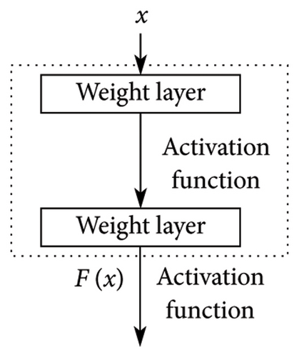
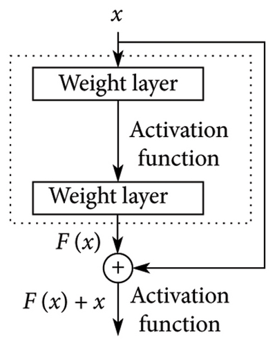
In Figure 3, the differences between a standard CNN block and a ResNet block are illustrated. In a standard CNN block, the input x undergoes a sequence of layers, producing a transformed output F(x). This output is then directly passed to the next activation function. On the other hand, within a residual block, there is an additional shortcut step. Instead of directly forwarding F(x) to the following activation function, it is combined with the initial input x, giving F(x) + x. This combined output then moves on to the next activation function. This additional step, where some layers are bypassed, is the defining characteristic of the residual block in ResNet.
Numerical study employs a standard CNN for the task of structural damage detection, owing to the relatively well controlled environment for data generation. However, when faced with the complexities of a real-world experimental test, the architecture of the network model shifts to a ResNet to ensure an enhanced performance.
The developed approach for structural damage identification combines the advantages of the phase space matrix and CNN. This method exhibits the robustness under the measurement noise and modeling uncertainty. Additionally, it is economical as it requires only a minimal number of sensors. The two advantages of the developed approach are demonstrated in the following sections on numerical analyses and experimental validations.
2.4. Nonprobabilistic CNN
While the combination of phase space matrix and CNN can handle noisy data, it still falls short in analyzing uncertainties comprehensively. Interval analysis offers a robust framework to account for the inherent uncertainties. The interval model, a prevalent mathematical framework, is commonly used to characterize structural uncertainty factors. Within this model, each element of the interval set signifies a potential realization of an uncertain event. Notably, constructing the interval model necessitates only the specification of upper and lower bounds for these uncertain factors, obviating the need for detailed internal mathematical or statistical distributions [44]. This simplification underscores its practicality.
When considering uncertainty, each parameter in the engineering structure exists within a certain range. An indicator can be proposed that when this range indicator reaches a certain value, it can be considered that the structure is likely damaged. When ESP is defined as α, ESP of a damaged structural element as αd, ESP of an undamaged structural element as αu, a two-dimensional space can be created for a structural element k, as shown in Figure 4. This space is formed by poltting its damaged ESP values (αdk) and undamaged ESP values (αuk) along two separate axes. The representation of a solid rectangle signifies the variation across both intervals. This rectangle is intersected by the failure plane, where αuk is equal to αdk. The terms and , respectively, represent the lower and upper bounds of αdk, while and , respectively, denote the lower and upper bounds of αuk.
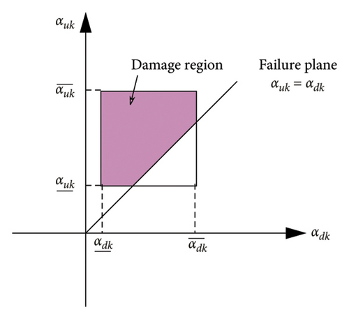
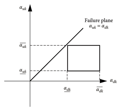
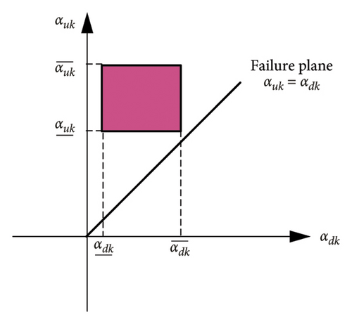
As the relative position of the rectangle and the failure plane shifts, the value of PoDE varies within the range of 0%–100%. Figure 4 illustrates the scenario where the PoDE value spans from 0% to 100%, whereas Figure 5 shows the situations where the PoDE is at its lowest point of 0% and its highest point of 100%. The PoDE reaches 0% when , and it attains 100% when .
In the context of the proposed approach using phase space matrix and CNN for structural damage identification, it becomes necessary to train two separate networks to account for uncertainties, employing interval analysis as the underlying methodology. As indicated in Table 1, when taking into account the upper and lower bounds of uncertainties from various sources, the network input is determined by adding and subtracting the respective ranges of uncertainties. In Table 1, the abbreviation PSM, which stands for phase space matrix, refers to the input data fed into the network. The variable ω represents the level of uncertainty in the input data, with distinct values of uncertainties for phase space matrix. All different types of uncertainties, including but not limited to measurement errors and finite element model discrepancies, are consolidated into a single unified factor. These uncertainties are then reflected in the variations of the input phase space matrix.
| Model | Input | Output |
|---|---|---|
By employing undamaged data and damaged data as inputs for and , respectively, four distinct datasets can be obtained, as shown in Figure 6. The “undamaged data” mean data generated from the initial state, representing the baseline of the structure, while the “damaged data” refer to the data of the state awaiting evaluation. Based on the diagram, for a structural element k, once its four unique values under different interval bounds are acquired, the PoDE value can be derived following the guidance provided in Figure 4 and based on equation (4).

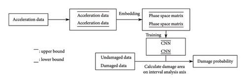
The proposed approach employs acceleration data to obtain phase space matrix as CNN input, and then interval analysis is adopted to calculate damage probability. The flowchart of the proposed approach is shown in Figure 7.
3. Numerical Studies
Numerical studies are conducted to verify the proposed approach by using the phase space matrix–based CNN and nonprobabilistic method to consider uncertainties. This section comprises details on the finite element model, data generation process, architecture of the developed CNN model, and the results of damage detection that account for structural uncertainties. Uncertainties from various sources, such as measurement noise and modeling errors, are consolidated into a singular entity and are reflected in the variations of the input phase space matrix.
3.1. Numerical Structure and Finite Element Model
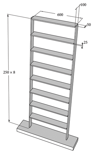
The efficacy of the proposed approach is demonstrated using a numerical model of an eight-story shear-type steel frame. The dimensions of the frame model are depicted in Figure 8. This steel structure stands at a height of 2000 mm and spans a width of 600 mm. The floor of each story is fabricated from thick steel plates measuring 100 mm × 25 mm. Each story comprises two columns, both having a consistent cross-sectional width of 50 mm and thickness of 5 mm. The beams and columns are cohesively welded to establish rigid connections. The base of these two columns is welded to a robust, solid steel plate, which is affixed to the strong floor. The initial Young’s modulus of the steel material is estimated at 200 GPa, and it has a mass density of 7850 kg/m3. Within the finite element model, each story is represented as an individual element. The weight of every story is concentrated and applied to a singular node, with only the vertical displacement taken into account. Consequently, the numerical model is constituted of 8 elements and 8 nodes.
3.2. Data Generation
Dynamic analysis is carried out on the baseline finite element model to produce training datasets for both input and output. The time-domain acceleration response for each node is captured. As previously mentioned in Section 2, the phase space matrix is formed using these acceleration data. The constructed phase space matrix is then taken as the input for the following analysis.
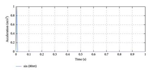
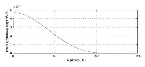
The methodology described in Section 2.1 provides the selection of parameters for phase space reconstruction. According to this methodology, the delay t is fixed at 1, and the dimension m is set to 16. In order to make the most of the architecture for computation and optimize both speed and accuracy, the data length is set as 210 = 1024. This results in the phase space matrix having a dimension of 16 × 1024. It is important to emphasize that the acceleration response data of each node are normalized. This step ensures that the results are not affected by variations in pulse amplitudes or any unusual data samples. The range of output ESP values is defined between 0 and 1. A value of 1 indicates that the structural element is under the initial state, whereas a value of 0 indicates that it is fully damaged.
Multiple damage case is explored for the damage modeling. Damage in the numerical steel frame are represented by reductions in the stiffness of structural elements. Two random elements are chosen to simulate structural damage. The damage level for these elements is varied from 0% (no damage) up to 30%, increasing with a 1% interval, namely, 1%, 2%, …, 30%. As a result, a total of 26,908 datasets are generated based on the finite element model analysis, which are then used for training, validation, and testing purposes.
3.3. CNN Architecture and Performance of the Proposed Approach
Before setting up a nonprobabilistic network, a deterministic CNN model is trained. This helps in determining the best network hyperparameters and ensures that the network is capable of performing the task of structural damage identification. The architecture of the neural network is detailed in Table 2. In the output shape of a convolutional layer, the first dimension indicates the batch size. The placeholder “−1” denotes that the batch size can vary, depending on the actual input data size. The next three dimensions represent the number of channels, height, and width of the input data, respectively. The developed CNN model consists of multiple convolutional layers. Each of these layers is paired with batch normalization, ReLU activation functions, dropout measures to avoid overfitting, and zero padding to keep the spatial dimensions intact after the convolution. The first convolutional layer has 64 output channels and uses a kernel of size (16 × 1). After this layer processes the data, batch normalization levels the outputs, the ReLU activation function adds nonlinearity, dropout measures help counteract overfitting, and zero padding makes sure that the spatial dimensions remain unchanged.
| Layer (type and number) | Output shape | Kernel size | Parameters |
|---|---|---|---|
| ReLU-1 | [−1, 1, 16, 1024] | 0 | |
| Conv2d-2 | [−1, 64, 1, 1024] | (16, 1) | 1088 |
| ZeroPad2d-3 | [−1, 64, 16, 1024] | 0 | |
| BatchNorm2d-4 | [−1, 64, 16, 1024] | 128 | |
| ReLU-5, dropout-6 | [−1, 64, 16, 1024] | 0 | |
| MaxPool2d-7 | [−1, 64, 8, 512] | (2, 2) | 0 |
| Conv2d-8 | [−1, 256, 1, 512] | (8, 1) | 131,328 |
| ZeroPad2d-9 | [−1, 256, 8, 512] | 0 | |
| BatchNorm2d-10 | [−1, 256, 8, 512] | 512 | |
| ReLU-11, dropout-12 | [−1, 256, 8, 512] | 0 | |
| MaxPool2d-13 | [−1, 256, 4, 256] | (2, 2) | 0 |
| Conv2d-14 | [−1, 256, 1, 255] | (4, 2) | 524,544 |
| ZeroPad2d-15 | [−1, 256, 4, 256] | 0 | |
| BatchNorm2d-16 | [−1, 256, 4, 256] | 512 | |
| ReLU-17, dropout-18 | [−1, 256, 4, 256] | 0 | |
| MaxPool2d-19 | [−1, 256, 2, 128] | (2, 2) | 0 |
| Conv2d-20 | [−1, 256, 1, 127] | (2, 2) | 262,400 |
| ZeroPad2d-21 | [−1, 256, 2, 128] | 0 | |
| BatchNorm2d-22 | [−1, 256, 2, 128] | 512 | |
| ReLU-23, dropout-24 | [−1, 256, 2, 128] | 0 | |
| MaxPool2d-25 | [−1, 256, 1, 64] | (2, 2) | 0 |
| Conv2d-26 | [−1, 64, 1, 63] | (1, 2) | 32,832 |
| ZeroPad2d-27 | [−1, 64, 1, 64] | 0 | |
| BatchNorm2d-28 | [−1, 64, 1, 64] | 128 | |
| ReLU-29 | [−1, 64, 1, 64] | 0 | |
| Linear-30 | [−1, 100] | 409,700 | |
| ReLU-31, dropout-32 | [−1, 100] | 0 | |
| BatchNorm1d-33 | [−1, 100] | 200 | |
| Linear-34 | [−1, 50] | 5050 | |
| ReLU-35, dropout-36 | [−1, 50] | 0 | |
| BatchNorm1d-37 | [−1, 50] | 100 | |
| Linear-38 | [−1, 8] | 408 |
Following this, a max pooling step is added to reduce the spatial dimensions, with a kernel size and stride of 2. This pattern continues in the next layers, but with changes in the number of output channels, kernel sizes, and the amount of zero padding used. The last convolutional layer in this section has 64 output channels and uses a kernel of size (1 × 2). The output from the CNN layers is then flattened into a one-dimensional vector, which becomes the input to the subsequent fully connected layers. These layers also include ReLU activation, dropout measures, and batch normalization. The first fully connected layer has 100 output units, the second has 50 output units, and the final fully connected layer has 8 output units corresponding to the number of structural elements.
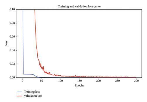
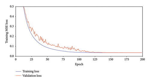
By introducing nonlinearity with ReLU activation, the network can effectively capture complex patterns from the data. The use of dropout regularization further equips the network to have a better generalization capability. Specifically, dropout rates set at 0.5 for the CNN section and 0.9 for the fully connected layers mean that during training, 50% and 90% of the activations are turned off randomly. This method helps the model avoid becoming overly dependent on specific neurons, pushing it to develop a broader and robust understanding of the data. The preprocessed dataset is randomly divided into training, validation, and testing subsets in accordance with the respective ratios of 70%, 15%, and 15%. Within the CNN architecture, the MSE is employed as the primary loss function, recognized for its robust application in evaluating regression models. The MSE calculates the mean value of squared discrepancies between the predicted outcomes and the actual damage labels of the model. In Figure 10, the training and validation loss curves for the scenario without uncertainty are depicted.
In this research, the R-squared (R2) value is adopted to investigate the efficacy of the proposed CNN model. The selection of R2 value is owing to its ability to quantify the proportion of the dependent variable variance influenced by the predictors of the model. In the context of structural damage identification, the R2 value effectively quantifies the CNN model’s prediction in correlating input matrix attributes with the output damage. R2 also presents a normalized metric to compare models from different studies. The R2 value spans from 0 to 1. Values close to 1 mean that the model fits the data well, showing that it predicts accurately. Conversely, a low R2 value close to 0 suggests that the model is unable to explain the variability in the dependent variable, indicating that the model might need improvements.
In Table 3, the efficacy of the proposed structural damage identification method is detailed across scenarios with different sensor counts and distinct levels of uncertainty (the uncertainty is simulated by adding a Gaussian distribution to the stiffness parameters of the finite element model). Scenarios 1.1 and 1.2 represent conditions without uncertainty, where Scenario 1.1 uses only one sensor, and Scenario 1.2 uses all eight sensors. Conversely, Scenarios 2.1 and 2.2 introduce a 1% uncertainty level; Scenario 2.1 utilizes a single sensor, while Scenario 2.2 employs all eight sensors. In both Scenario 1.1 and Scenario 2.1, the single sensor employed is installed on the first floor of the steel frame. Notably, the R2 values remain nearly consistent whether the data are sourced from all eight sensors or a single one. This observation highlights the capacity of proposed CNN model to identify and represent the inherent correlations between input data and damage status, even in situations where the sensor data are limited. A comparison is conducted between two methods: the proposed approach that uses the phase space matrix as input for the CNN and another that relies on raw time series data. The distinguishing factor between these two CNN models is their input data types and the associated convolutional kernel size.
| Uncertainty level | Input data source | Sensor number | Training MSE | Validation MSE | Validation subset R2 | Testing subset R2 | |
|---|---|---|---|---|---|---|---|
| Scenario 1.1 | 0 | Single sensor | 1 | 6.40e − 06 | 7.23e − 04 | 0.996 | 0.996 |
| Scenario 1.2 | 0 | Eight sensors | 1–8 | 5.63e − 06 | 6.12e − 04 | 0.997 | 0.996 |
| Scenario 2.1 | 1% | Single sensor | 1 | 1.11e − 05 | 4.44e − 03 | 0.978 | 0.977 |
| Scenario 2.2 | 1% | Eight sensors | 1–8 | 1.07e − 05 | 4.18e − 03 | 0.978 | 0.977 |
In Table 4, a distinct performance difference across two test scenarios is demonstrated. When no uncertainty is present, an R2 score of 0.991 is achieved by the CNN model using the raw time response. However, upon the introduction of uncertainty, a decline in performance is observed, with an R2 score dropping to 0.966 in Scenario 2. In contrast, consistent performance is exhibited by the CNN using phase space matrix as input, with R2 values of 0.997 and 0.977, respectively, without and with uncertainty effect, indicating a greater robustness to uncertainties when using the phase space matrix as input rather than the raw time responses.
| Uncertainty | Sensor number (1–8) | Testing subset R2 of CNN using raw time responses | Testing subset R2 of CNN using phase space matrix | |
|---|---|---|---|---|
| Scenario 1.1 | 0 | 1 | 0.991 | 0.996 |
| Scenario 2.1 | 1% | 1 | 0.966 | 0.977 |
In Figure 11, damage level identification outcomes for various instances within Scenario 1 are illustrated. Figures 11(a), 11(b), 11(c), 11(d) display the identification results for testing datasets No. 2, No. 4, No. 8, and No. 11, respectively. The element number is depicted on the x-axis, while the damage level is represented on the y-axis. True damage levels are denoted by blue bars, whereas the predicted damage levels are indicated by red bars. These depictions underscore the proficiency of the proposed methodology in identifying the accurate damage levels.
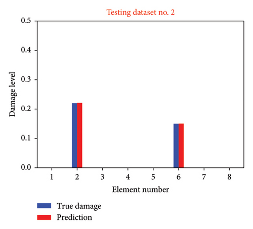
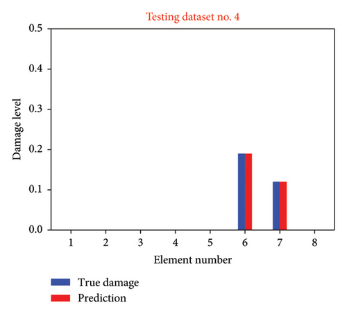
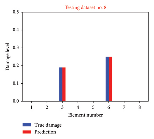
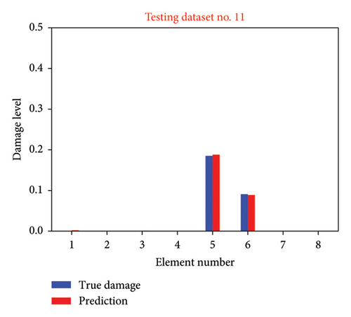
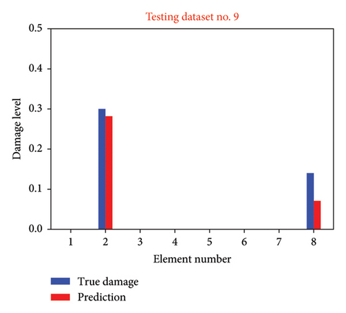
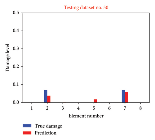
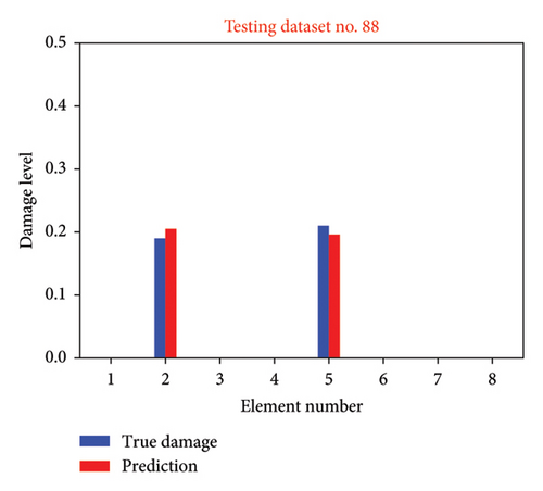
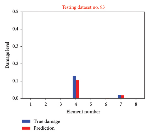
Figure 12 shows the damage identification results for multiple cases within Scenario 2 (1% uncertainty level). Figures 12(a), 12(b), 12(c), and 12(d) illustrate the identification results for testing datasets No. 9, No. 50, No. 88, and No. 93, respectively. It is evident that the network retains its ability to predict damage, but there is a marked reduction in its accuracy relative to previous observations. Specifically, in the prediction for minor damage in testing dataset No. 50, undamaged element No. 5 is identified as damaged. The identified damage levels of elements 1 and 6 are underestimated. To address the decline in damage detection performance under conditions of uncertainty, the nonprobabilistic phase space matrix–based CNN is applied.
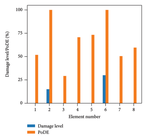
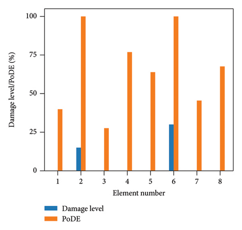
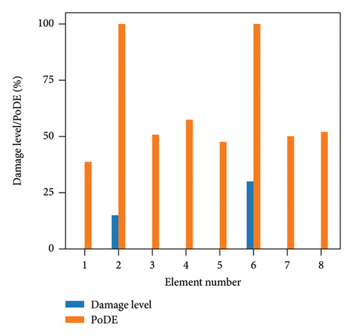
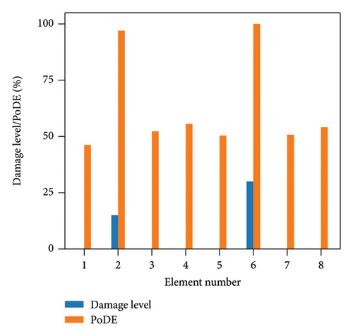
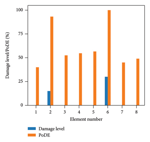
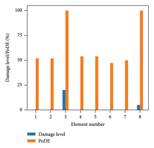
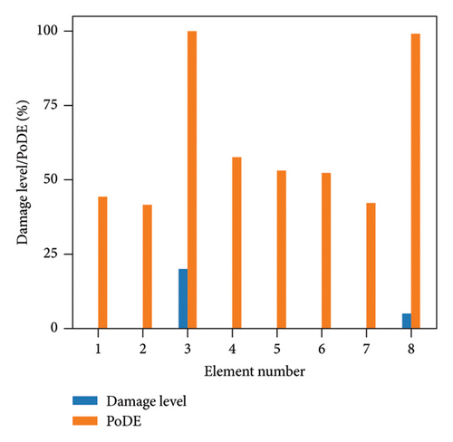
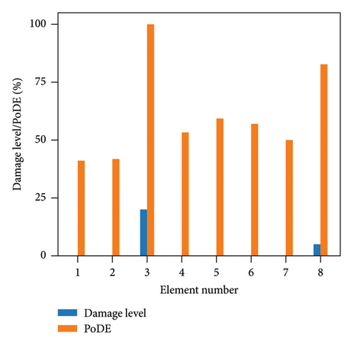
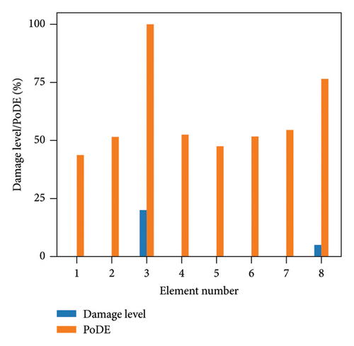
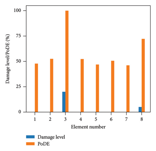
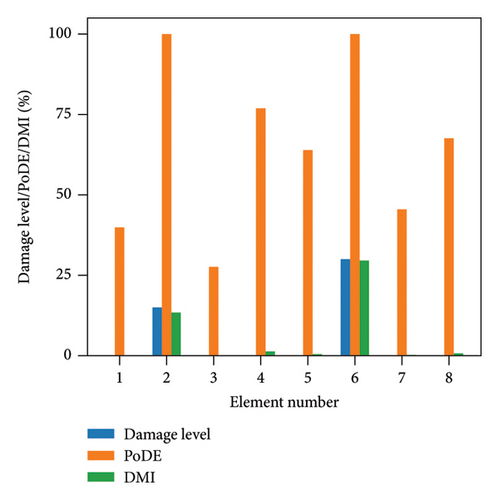
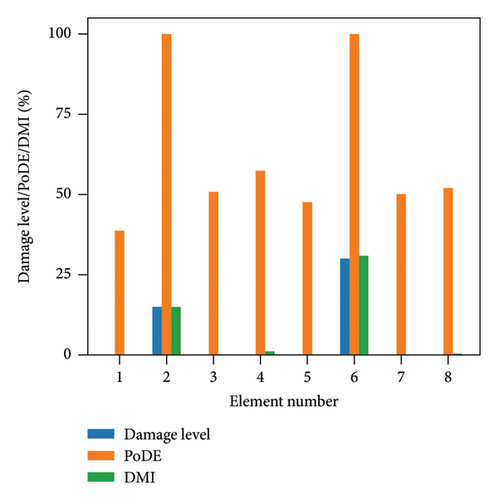
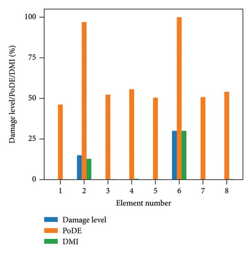
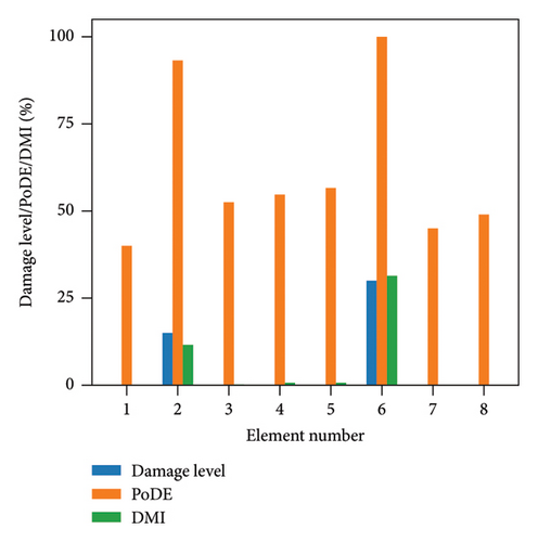
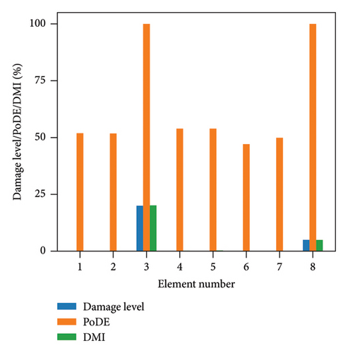
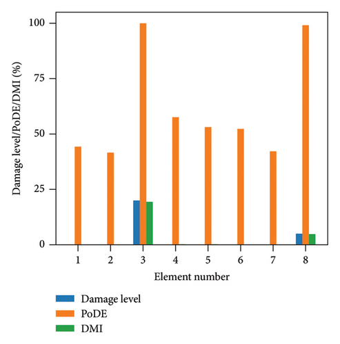
To demonstrate the effectiveness of the proposed approach, as shown in Table 5, two damage cases are selected for study. Damage case 1 involves 15% damage in element No. 2 and 30% damage in element No. 6, with no damage in the other elements. Damage case 2 has 20% damage in element No. 3 and a minor 5% damage in element No. 8. To assess the performance of the proposed method under varying levels of uncertainty, each damage case has 5 subscenarios, considering uncertainty levels of 2%, 3%, 5%, 8%, and 10%, respectively, to evaluate the identification results of the presented approach. In the interval analysis, uncertainty is realized by directly augmenting or diminishing the input signal by a specified level as indicated in Table 1. For example, when the uncertainty level is set as 5%, the acceleration responses employed for the lower and upper bounds should be adjusted to 95% and 105% of the raw data, respectively. Then the adjusted responses would be embedded to reconstruct phase space matrices.
| Element number | Case 1 | Case 2 |
|---|---|---|
| 1 | 0 | 0 |
| 2 | 15% | 0 |
| 3 | 0 | 20% |
| 4 | 0 | 0 |
| 5 | 0 | 0 |
| 6 | 30% | 0 |
| 7 | 0 | 0 |
| 8 | 0 | 5% |
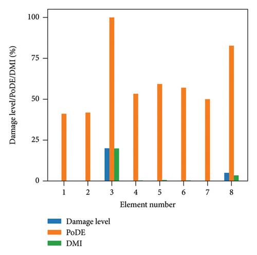
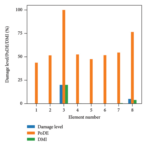
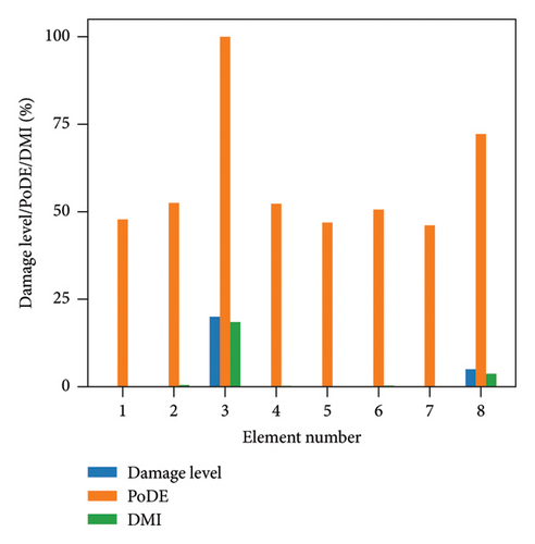
Figure 13 illustrates the damage identification results for Case 1, taking into account various uncertainty levels. Represented by blue bars, the damaged elements exhibit PoDE values nearing 100%. These values are significantly higher than those of the undamaged elements, indicating a strong probability that these elements are indeed damaged. Figure 14 shows the results for Case 2, despite the presence of minor damage levels coupled with high uncertainty. The PoDE for element No. 8 is quite high, leading to the inference that element No. 8 is damaged. It is observed that the PoDE values of undamaged elements are nonnegligible, even though their PoDE values are considerably lower than those of the damaged elements. This indicates that PoDE may overestimate the probability of damage. Consequently, the introduction of the DMI value becomes essential to assess the damage level more accurately. In Figures 13(a) and 13(b), some relatively high levels of PoDE values are observed. It should be noted that the identified damage levels of these elements with relatively large PoDE values are very minor. Therefore DMI is used to indicate both the damage level and probability.
In Figures 15 and 16, the damage predictions for Case 1 and Case 2 incorporating DMI are illustrated. It is evident that DMI can accurately indicate the level of structural damage. Notably, even under a high uncertainty level of 10%, DMI still precisely identifies minor damage and ensures no false identification of undamaged elements as damaged, which is otherwise observed in Figure 15(e).

4. Experimental Studies
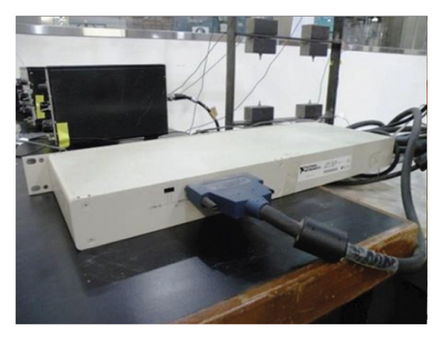
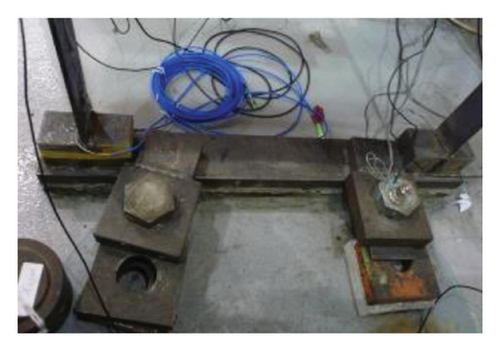
Experimental studies are conducted to further validate the performance of the proposed approach. In the laboratory, a steel framework consisting of seven floors is manufactured to investigate the effectiveness of the proposed approach for damage identification of structures. Figure 17 shows the overview, boundary conditions, and data acquisition system of the steel frame during the experimental tests in the laboratory.
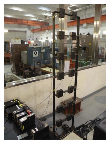
Numerical data generated from a finite element model with 70 elements are used for training and validation. The initial model updating is conducted based on identified vibration characteristics [46] before data generation. This updating process involves two stages. In the first round, the elastic modulus of structural elements and the stiffness of support restraints are updated using the first-order modal sensitivity–based method. Experimental modal analysis is performed with hammer tests by employing eight sensors to extract natural frequencies and mode shapes, with the first seven modes used for the updating. The second round further refines the model using a dynamic response sensitivity method, adjusting the elastic modulus values based on measured dynamic response data from seven sensors under hammer excitations. High-frequency noise is filtered out with a low-pass filter, and Rayleigh damping is assumed.
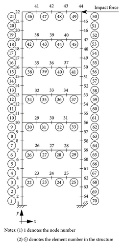
After training, the accuracy and performance of the proposed approach are verified with experimental data measured under the damaged state. This damage scenario includes 12.5% stiffness reductions at the 6th and 12th elements, as shown in Figure 18. Given a higher number of elements in the finite element model compared to numerical studies, more layers are required in the network model. Traditional CNNs may not converge efficiently due to this depth, and hence ResNet is chosen for the experiments because of its better handling of such complexities.

4.1. Data Generation
In Figure 19, an impact force is applied at node 44 in the x-direction to produce training datasets. These datasets are defined based on the updated finite element model of this steel frame structure with different structural conditions, representing undamaged, single, and double damage scenarios. A random impact force with a 1%–2% variance, based on the measured force from the tests, is introduced to simulate variations in the applied impact force for realistic simulations. Nine sensors are used on the frame structure to capture acceleration responses and are placed at locations 4x, 5x, 11x, 14x, 19x, 50x, 53x, 56x, and 59x, with “x” denoting x-direction acceleration. Sampling rate is set as 1000 Hz. 28,008 dataset samples are generated, wherein the stiffness reductions are randomly distributed across one or two elements. The maximum stiffness reduction in this scenario is capped at 30%.
Acceleration data from sensors are converted into a phase space matrix. Each sample becomes a matrix with nine channels, equating to the sensor number. With a delay of 13 and dimension set at 14, this matrix is structured based on the methodology described in Section 2, ensuring consistent transformation of raw data. The input has a (14 × 281 × 9) dimension, and the output contains seventy stiffness parameters for the steel frame. Data are split as 70% for training, 15% for validation, and 15% for testing. Additionally, lab-collected experimental acceleration data under the damaged state are used as extra testing dataset.
Initially, datasets without uncertainty are employed to train the deterministic network, which aids in determining the hyperparameters of the network. Subsequently, the performance of the deterministic network is evaluated using data with 10% uncertainty to gauge its robustness in scenarios with uncertainty. Lastly, the proposed approach is deployed for structural damage identification by using experimental data from damaged structure to assess its performance when taking uncertainty into consideration.
4.2. Architecture of Neural Networks Used in Experimental Verification
In the experimental study, a deep residual neural network (ResNet) is chosen to identify damage due to its capability to handle the steel frame model’s intricate, high-dimensional data. While the numerical model has only seven elements, the experimental structure simulates a detailed scenario with 70 elements. This complexity requires a deeper neural network. A standard CNN, although versatile, finds it challenging to converge with many convolutional layers, which is a hurdle present in our model. ResNet, with its ability to learn residual functions, effectively trains deeper networks and improves the performance of structural damage identification [47]. Table 6 details the architecture of the used ResNet with 35 residual blocks.
| Layers | Settings | Output size |
|---|---|---|
| Convolution | 1 × 15 Conv, strides = (1, 5) | 14 × 57 × 24 |
| Residual block (1–11) | Batch normalization, tanh | 14 × 57 × 24 |
| 2 × 5 Conv, strides = (1, 1) | ||
| Batch normalization, tanh | ||
| 2 × 5 Conv, strides = (1, 1) | ||
| Shortcut | ||
| Residual block (12–23) | Batch normalization, tanh | 7 × 28 × 168 |
| 2 × 5 Conv, strides = (1, 1) | ||
| Batch normalization, tanh | ||
| 2 × 5 Conv, strides = (1, 1) | ||
| Shortcut | ||
| Residual block (24–35) | Batch normalization, tanh | 3 × 14 × 312 |
| 2 × 5 Conv, strides = (1, 1) | ||
| Batch normalization, tanh | ||
| 2 × 5 Conv, strides = (1, 1) | ||
| Shortcut | ||
| Regression layer | Batch normalization, tanh | 1 × 1 × 312 |
| 3 × 14 global average pooling | ||
| Dense layer | 70 × 1 fully connected, tanh | 70 |
4.3. Damage Identification Results
| Prediction on the 6th element (%) | Prediction on the 12th element (%) | Training subset R2 | Validation subset R2 | |
|---|---|---|---|---|
| No uncertainty | 13.49 | 11.20 | 0.948 | 0.926 |
| 10% uncertainty | 16.61 | 2.75 | 0.899 | 0.610 |
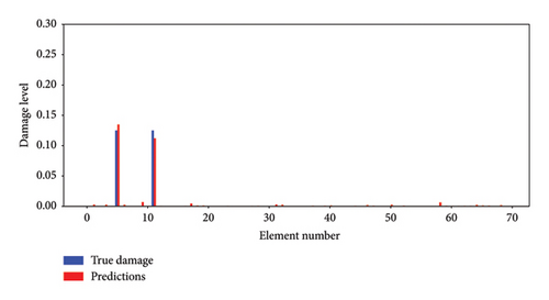
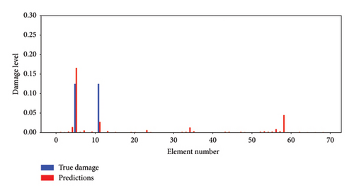
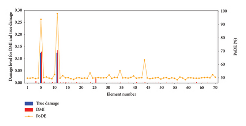
Following the methodology in Section 2, the proposed nonprobabilistic approach is employed for structural damage identification. The PoDE and DMI values are shown in Figure 22. From the figure, it is evident that the PoDE values of the damaged elements are approximate to 100%, and the DMI values also accurately identify the level of the damage. The experimental results indicate that the proposed method can precisely provide both the probability of damage and identify the level of damage, even in a high-uncertainty environment.
5. Conclusions and Discussion
A nonprobabilistic structural damage identification method based on phase space matrix, CNN, and interval analysis is proposed in this article. The methodology demonstrates promising capabilities for applications in structural health monitoring, maintaining efficacy even under high-uncertainty environments. The identification results of the numerical simulations on an eight-story shear-type steel frame model and experimental tests on a seven-story steel frame demonstrate that the proposed approach achieves a high accuracy in detecting and quantifying damage severities of multiple damage cases. To validate the effectiveness of the proposed method under uncertainty, PoDE and DMI are employed to identify the probability of damage and the level of damage.
The proposed approach addresses several challenges. The results show that in a high-uncertainty environment, deterministic networks may not extract effective features from data to predict damage. In contrast, the proposed approach still maintains a high accuracy. Moreover, since the phase space–based method requires only a few sensors to identify structural damage, the proposed nonprobabilistic approach is cost effective and has potential to identify structural damage of real structures in engineering environments with a high uncertainty level.
Despite its strengths, the proposed approach still has some limitations. Interval analysis could not well consider the uncertainty correlation between variables. When analyzing multiple correlated variables, interval analysis may yield overly conservative results. Additionally, interval analysis struggles to handle coupling effects in dynamic systems and could not provide a quantified representation of uncertainties. Future studies will be conducted to consider the challenges. The applications of the proposed approach to large-scale structures will also be further conducted in future studies.
Conflicts of Interest
The authors declare no conflicts of interest.
Funding
The support from the Australian Research Council Discovery Projects (DP210103631), “AI Assisted Probabilistic Structural Health Monitoring with Uncertain Data,” is acknowledged.
Acknowledgments
The support from the Australian Research Council Discovery Projects (DP210103631), “AI Assisted Probabilistic Structural Health Monitoring with Uncertain Data,” is acknowledged.
Open Research
Data Availability Statement
The data used in this paper will be available upon reasonable request.


