Structural Damage Identification Based on Transfer Learning and Power Spectral Density
Abstract
This paper proposes a novel method for structural damage identification that integrates the power spectral density (PSD) of structural acceleration responses with densely connected convolutional networks (DenseNet). The method transforms the training object of the DenseNet into a numerical matrix (PSD matrix) for structural damage identification. Leveraging transfer learning, the DenseNet models are initially trained on simulated data and further fine-tuned using experimental data to enhance robustness and generalization. Results demonstrate that frequency-domain signals processed by PSD significantly enhance model performance, achieving lower mean squared error (MSE), higher Pearson’s correlation coefficient (R value), and reduced mean absolute error (MAE) compared to time-domain signals. The effectiveness of this method was verified on a six-story frame structure. This study underscores the efficacy of transfer learning in bridging the gap between simulated and real-world data, thereby facilitating effective structural health monitoring and damage identification.
1. Introduction
Structural health monitoring (SHM) is a critical technological approach used to assess the condition of various structural systems, including buildings, roads, and bridges. An essential aspect of SHM is structural damage identification, which plays a vital role in ensuring the safety of engineering structures. This process involves the accurate and efficient determination of the location and extent of damage. In recent years, vibration-based methods have become prevalent for this purpose due to their effectiveness in identifying structural anomalies [1–3]. In their study, Faravelli and Casciati [4] explores the potential of the response surface method in developing a statistical discriminant analysis approach, where not only the presence of damage but also its location can be inferred by comparing two approximations. Farrar, Doebling, and Nix [5] presents research on feature selection and the development of statistical models, applying these techniques to large-scale laboratory structures. Casciati [6] develops a method for damage detection and localization in time-variant structures using linear response surface models, where changes in statistical error characterization are linked to structural modifications and validated through experimental data from a structure with distributed cracking. However, one of the challenges with vibration-based methods is that the acquired time-domain signals often contain noise [7, 8], which can obscure the detection of structural damage. To address this issue, researchers have increasingly turned to various signal processing techniques to enhance the clarity and reliability of the data. Among these techniques, the power spectral density (PSD) function stands out as particularly significant [9, 10]. The PSD function transforms time-domain signals into frequency-domain signals, providing a clearer representation of the structure’s damage characteristics. This transformation facilitates a more detailed analysis by highlighting frequency changes that correspond to damage, thus improving the accuracy of damage detection in structural health monitoring systems.
Bayissa and Haritos [11] introduced a novel damage sensitivity parameter derived from the bending moment response power spectral density (MSD) for damage identification in two-dimensional plate structures. This parameter, referred to as the mean square value (MSV), encapsulates the total energy or average output power under the bending MSD pattern. It is quantified by the zero-order moments of the response spectral density, serving as the primary response parameter. Derived damage indices (DIs) such as the relative change in MSV, MSV curvature (MSVC), normalized damage indices, and relative root-mean-square error (RRMSE) facilitate the detection and localization of structural damage. Subsequent studies by Zheng et al. [12], Pedram, Esfandiari, and Khedmati [13], and Fallah, Hoseini Vaez, and Esfandiari [14] utilized a finite-element model correction method to evaluate the sensitivity of structural damage parameters by obtaining power spectral densities. Fang et al. [15] developed a substructure damage identification method predicated on power spectral density sensitivity analysis. This method treats the substructure as an independent entity and enabled structural damage identification on a six-layer frame model through model updating techniques. Kumar et al. [16] proposed an algorithm based on variations in PSD for detecting damage, predicting its location, and assessing its extent in reinforced concrete beams. Liberatore and Carman [17] determined the energy within the bandwidth near the resonance, which is highly sensitive to damage. This energy was quantified using its root MSV and, in conjunction with mode shapes, used to localize the damage. Nguyen [18] explored the alterations in PSD resulting from beam damage, employing vibration signals from damaged beams under moving loads to achieve damage detection in the structure.
While power spectral analysis offers precise identification of damage location and extent in structures, its application to large-scale structures is computationally demanding, and a significant amount of computational time and resources are usually required during the damage identification process. In recent years, deep learning has emerged as a versatile tool in numerous fields, including computer vision [19–21], signal processing [22–24], and medicine [25–27]. Its adoption in structural health monitoring [28–31] highlights a significant shift towards leveraging advanced machine learning techniques to enhance the efficiency and accuracy of damage identification processes in complex engineering systems.
Saleem et al. [32] employed image capture and convolutional neural networks (CNNs) for the detection of cracks in the wall and bridge structures at a laboratory scale. This innovative method integrates geo-referenced data derived from image capture and geo-tagging, utilizing a trained CNN to swiftly and accurately ascertain both the location and extent of structural damage. Further developments in the field were made by the researchers Song, Liu, and Yuan [33], Ye, Jin, and Chen [34], Protopapadakis et al. [35], Zhou et al. [36], and Modarres et al. [37], who leveraged the automatic learning capabilities of CNNs to develop a computer vision-based method for detecting concrete cracks. An advanced approach was proposed by Xu et al. [38], involving an enhanced, fused, CNN architecture. This architecture utilizes images captured by cameras, which serve as training, validation, and testing datasets. It is specifically designed for the identification of cracks in steel box girder bridges, addressing complex interference elements such as cracks, handwritten fonts, and backgrounds. Song, Sun, and Yuan [39] proposed a lightweight, deep CNN (DCNN) for crack pixel-level segmentation, utilizing drones to detect cracks on a large-span bridge. Chen et al. [40] generated time-frequency images from the original one-dimensional sensor signals using continuous wavelet transform (CWT). A DCNN was then employed to extract and analyze structural damage features from these time-frequency images to identify various structural damages.
While CNNs are proficient in detecting the location and extent of structural damage through image recognition, their application is predominantly limited to surface damage, omitting vital vibration data from the structure. This limitation hinders their ability to identify internal damage within structures. Recent advancements in research, as evidenced by studies [41–43], demonstrate that integrating structural vibration information with deep learning techniques can effectively address this shortfall. By combining these modalities, researchers have developed more comprehensive methodologies that enhance the capability of damage detection systems to identify both surface and internal structural damages.
Shu et al. [44] introduced a vision-based displacement estimation method, which leverages video data to extract structural displacement responses. Subsequently, structural damage identification is conducted using a model updating method. This approach allows for precise assessments of structural integrity based on observable displacements. Alazzawi and Wang [45] present a novel damage identification method for frame structures that integrates structural response signals with a deep residual network (DRN). This method effectively discriminates the size and localization of structural damage through the output structure of the DRN, demonstrating the network’s capability in processing complex data. Wang et al. [46] explores the potential of learning damage-related features from vibration characteristics, mapping these features to damage indicator labels. The effectiveness of this approach is validated through both simulations and experimental applications on a 7-story frame, showcasing its practical relevance. Abdeljaber et al. [47], Teng et al. [48], and Zhang et al. [49] discuss the use of a one-dimensional CNN for damage identification from the acceleration signals of a structure. This technique underscores the utility of leveraging signal processing within neural networks for structural analysis. He et al. [50] and Ghahremani et al. [51] combine a DCNN with a fast Fourier transform (FFT). This integration enables the DCNN to autonomously extract damage features from frequency information, enhancing the ability to identify structural damages effectively. This synergy between DCNN and FFT exemplifies the advancement in utilizing combined methodologies for more accurate damage detection.
While the integration of deep learning with structural vibration information has proven effective for comprehensive and efficient identification of structural damage, it presents notable challenges: (1) Deep learning-based structural damage identification typically requires extensive datasets to train CNNs. In practical engineering contexts, acquiring a complete dataset that encompasses various types of structural damage is often challenging [52–55]. This limitation can impede the training process and the subsequent performance of the CNNs, as they rely heavily on large, diverse datasets to achieve high accuracy and robustness. (2) The use of finite element model data for training and real measured data for testing presents another set of difficulties. This approach necessitates highly detailed finite element modeling to match the complexity of real structures, which can be both time-consuming and prone to errors. The discrepancies between modeled and actual data can significantly affect the reliability of damage identification.
To address these drawbacks, the application of transfer learning with CNNs offers a promising solution. Transfer learning can enhance the training effectiveness and detection accuracy of CNNs, particularly by improving their generalization ability. By transferring learned features from one domain to another, this method can effectively utilize pretrained networks on large datasets, thereby requiring fewer data from the specific engineering problem at hand. This approach not only mitigates the need for extensive damage-specific data but also helps in adapting the model to the nuances of real-world structures, leading to more accurate and reliable damage detection.
2. Related Work
The transfer learning technique, adept at transferring knowledge from the source domain to the target domain, has emerged as a highly promising method for structural damage identification. In the realm of structural health monitoring, transfer learning has already demonstrated significant success in detecting surface defects on structures [56–61]. This paper enhances the methodology by integrating structural vibration data with transfer learning. We utilize datasets generated by finite element models for training and subsequently fine-tune the CNN model with a limited number of real structural samples to tailor the model for the specific task of damage identification in real-world structures.
The main contributions of this paper are outlined as follows: (1) We utilize the PSD function in combination with a CNN using a limited number of accelerometers for structural damage identification. (2) The signal processed using PSD results in a higher accuracy of the CNN model compared to the time-domain acceleration signal. (3) We examine complex detection scenarios, including two-element damage, three-element damage, and the impact of noise, to validate the robustness of our damage identification approach. (4) We apply transfer learning techniques to adapt CNN models, initially trained with simulated data, to real-world data, enhancing their practical applicability. (5) We validate the effectiveness of our method through laboratory models.
The paper is structured as follows: Section 3 delineates the research methodology; Sections 4 and 5 provide numerical and experimental evaluations of the proposed methodology, respectively; and Section 6 concludes with a discussion of the findings and implications of this research.
3. Methodology
In this paper, we initiate our methodology by collecting acceleration response data from a finite element model. This time-domain signal is transformed into a frequency-domain signal using the PSD function [62]. We then compute the power spectral difference between the damaged and undamaged structures. This difference is converted into a numerical matrix, which serves as the training data for the CNN. To enhance the model’s applicability to real-world scenarios, the network undergoes further training with a small dataset comprising power spectral difference data from actual structures. For the implementation of our methodology, we employ a three-dimensional dense CNN (DenseNet) [63]. This architecture is chosen for its efficacy in feature extraction through its densely connected layers, which facilitate learning complex patterns in the data, crucial for accurate damage identification.
3.1. The Application of PSD Function and DenseNet in This Method
In the simulation phase of the application, as shown in Figure 1, the first step is the creation of the dataset. We apply an impact force in a specific direction to a node of the structure and collect acceleration data from the corresponding sensors. Subsequently, we calculate the PSD of these acceleration data and compute the difference between the PSDs of the damaged and undamaged structures. The data are divided into three parts: 70% for training the DenseNet model, 15% for validation, and 15% for testing. Once training is complete, the DenseNet model is exported, and the testing dataset is imported into the model to obtain damage recognition results. To ensure the generalization ability of the CNN and account for variations in the applied impact force during the experiment, we used a random impact force ranging from 90 N to 110 N. This procedure highlights the application of PSD and DenseNet in our method, with specific experimental details outlined in the migration learning method (i.e., Section 3.3).

3.2. Transfer Learning
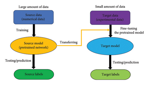
Transfer learning (as shown in Figure 2) is a technique derived from deep learning where the principal objective is to leverage knowledge acquired from one task (source task) to enhance the learning efficiency and performance on a related but distinct task (target task). This process typically involves the following steps: (1) Select a source task: Identify a task that is closely related to the target task and train a model on it until it achieves satisfactory performance. This model learns features that are potentially beneficial for both tasks. (2) Migrate the model to the target task: Transfer the weights from the trained model on the source task to a new model dedicated to the target task. This step avoids the need for training from scratch and uses the pretrained model as a starting point. (3) Fine-tune the model: Adapt the model to the target task by retraining it, either fully or partially, on the target task’s data. This is crucial for making the model more relevant to the specific characteristics of the new data. (4) Evaluate and adjust: Assess the model’s performance on the target task. Based on the outcomes, further refine or adjust the model’s parameters to optimize its accuracy and effectiveness.
3.3. Advantages of the Proposed Methodology
In this paper, we exploit the synergy between the PSD function and transfer learning to enhance the training of DenseNet, a CNN. We begin by pretraining the model using simulated data from the source domain, followed by retraining the model using transfer learning techniques with a select dataset from experimental studies as the target domain. The advantages of this method are as follows: (1) The integration of the PSD function with DenseNet: By using frequency domain signals as the training target, this approach enhances the efficiency of the neural network during the training process, optimizing learning outcomes. (2) The application of transfer learning techniques: This methodology ensures that the neural network model is not overly fitted to simulation data, thereby maintaining robust performance in real-world applications.
4. Numerical Simulation
4.1. Model Parameters
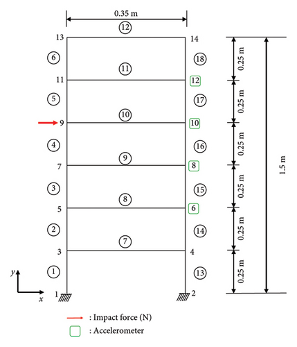
As shown in Figure 3, the frame structure consists of 14 nodes and 18 elements, each with three degrees of freedom (two translational and one rotational). The structure has dimensions of 0.35 m in width and 1.5 m in height, with two distinct density values: 2750 kg/m3 for elements 1 through 6 and 7850 kg/m3 for elements 7 through 18. It possesses an elastic modulus of 2.1 × 10¹¹ Pa and a Poisson’s ratio of 0.3. Accelerations in the x-direction were measured at nodes 6, 8, 10, and 12. To evaluate the generalization ability of the CNN model, a random impact force, ranging from 90 to 110 N, was applied at node 9 in the x-direction.
4.2. Data Generation
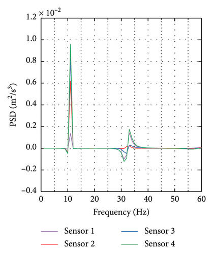
When an impact force is applied, the acceleration response from four designated nodes is captured at a sampling rate of 2000 Hz. The PSDs of these responses are calculated for both undamaged and damaged structures, and then, their difference is calculated. For the damage scenarios, we consider up to three elements as damaged. Damage is simulated as a reduction in the cross-sectional area of an element, effectively decreasing its stiffness. This reduction ranges from 0% to 50%, with intervals of 1%. Each damage scenario is simulated 10 times for each element (where the impact force applied to each damage scenario is randomized, with the aim of enhancing the generalization ability of the CNN model). The data are then split, with 70% used for training the CNN, 15% for validation, and 15% for testing. To assess the robustness of the methodology, noise levels of 3 dB S/N and 5 dB S/N are added to each damage scenario.
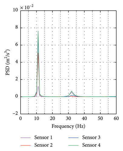
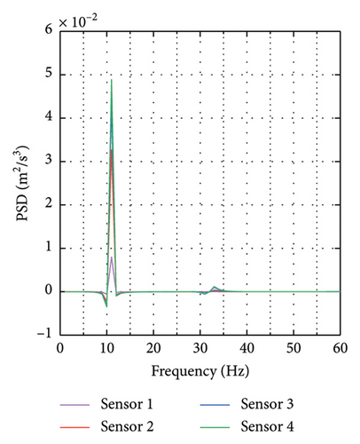
To illustrate the variations in the PSD across different damage scenarios, we performed data visualizations as presented in Figure 4. Figure 4 focuses on the power spectrum of a frame structure: Figure 4(a) displays the power spectrum data of the frame when undamaged; Figure 4(b) shows the power spectrum difference for a frame element with 25% damage on element 5; Figure 4(c) depicts the power spectrum difference for a frame element with 15% damage on element 10.
4.3. Performance Evaluation
We employ mean square error (MSE) and mean absolute error (MAE) as metrics to quantify the discrepancies between the predicted outputs and the actual damage values. Additionally, Pearson’s correlation coefficient (denoted as R, with a range of −1 to 1) is utilized to evaluate the predictive accuracy of the training model. Pearson’s correlation coefficient measures the linear relationship between the true labels and the predicted outputs, providing a statistical basis for assessing the model’s performance in terms of its linearity and directionality.
4.3.1. MSE
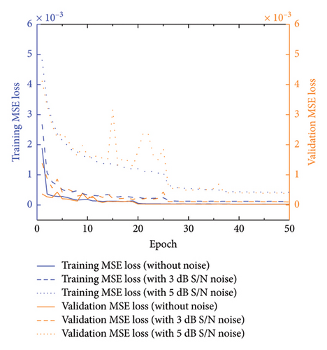
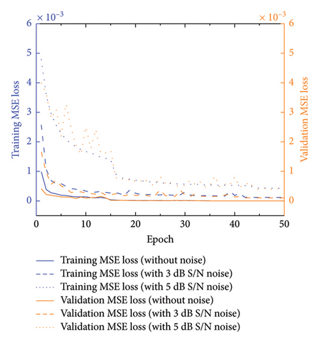
In the figure, the horizontal coordinate ‘Epoch’ refers to the training process during which the model learns from the entire training dataset in one complete iteration. Figure 5(a) compares MSE values under three conditions of single-element damage: no added noise, 3 dB S/N noise, and 5 dB S/N noise. Despite the introduction of noise, the model maintains high accuracy, with only a slight performance decline observed at noise levels of 3 dB S/N (MSE = 1.0 × 10⁻⁴) and 5 dB S/N (MSE = 4.6 × 10⁻⁴). Figure 5(b) further explores the model’s performance under scenarios of damage involving multiple elements, illustrating the robustness of the training process to complex damage patterns.
4.3.2. R Value
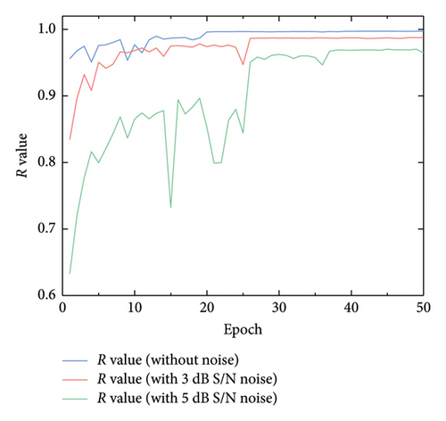
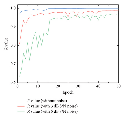
The variations in the R value across different scenarios are detailed in Figure 6, with Figure 6(a) showing variations for single-element damage cases and Figure 6(b) comparing results under scenarios of multiple-element damage. Remarkably, even with the inclusion of a 5 dB S/N noise, the lowest R value observed was 0.964, highlighting the model’s robustness.
4.3.3. MAE
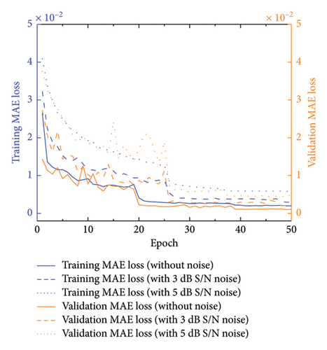
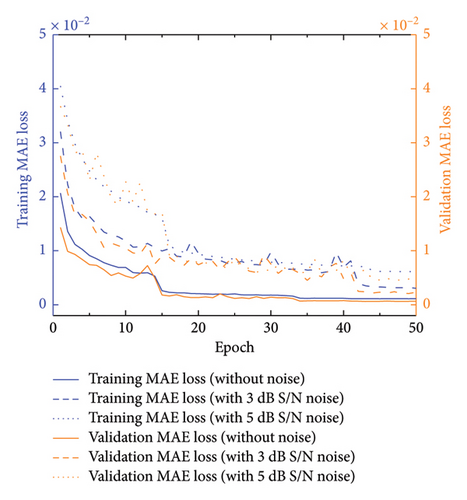
Additionally, the MAE was utilized to gauge the model’s accuracy, as depicted in Figure 7. The MAE exhibits a decreasing trend during training, indicating consistent high accuracy of the model even under varying noise conditions.
4.3.4. Model Accuracy and Error Performance
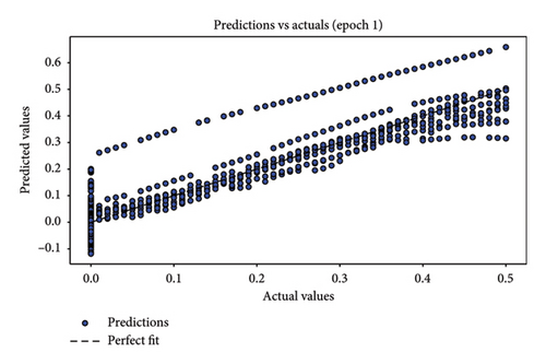
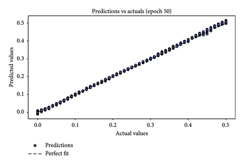
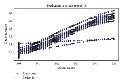
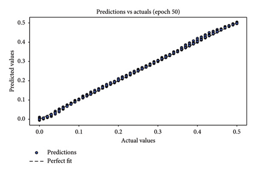
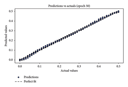
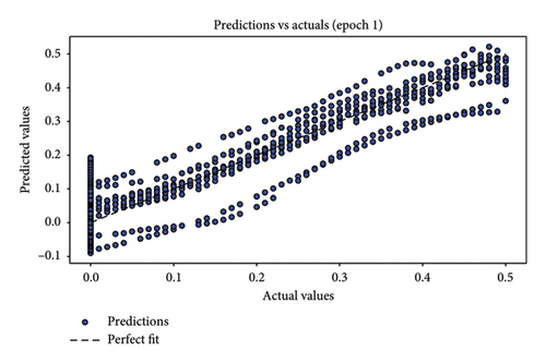
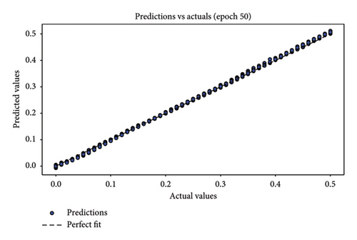
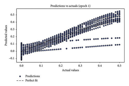
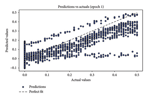
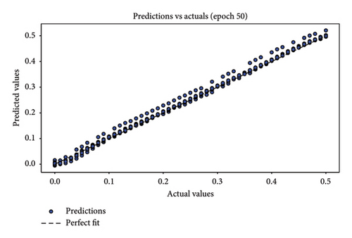
In assessing the accuracy of the developed model, relying solely on a single metric is insufficient. Hence, it is crucial to consider the collective insights from multiple evaluation metrics. The results of model relevance, depicted in Figures 8 and 9, showcase the outcomes from the final iteration of the training process. Initially, at the end of the first training session, the scatter plot points are widely dispersed, indicating a low accuracy. However, as the training progresses through 50 rounds, the regression line increasingly aligns closely with the data points, demonstrating significant improvements in model accuracy. Figures 8(a), 8(c), and 8(e) depict the first iteration prediction plots for a framed structure under single-element damage scenarios with varying noise conditions: no noise, 3 dB S/N noise, and 5 dB S/N noise, respectively. Conversely, Figures 8(b), 8(d), and 8(f) show the prediction maps from the last iteration for the same scenarios and noise settings. Similarly, Figures 9(a), 9(c), and 9(e) present the first iteration prediction plots for the multiple-element damage case without noise, with 3 dB S/N noise, and with 5 dB S/N noise, respectively. Figures 9(b), 9(d), and 9(f) display the last iteration prediction plots for the multidamage case under the corresponding noise conditions: no noise, 3 dB S/N noise, and 5 dB S/N noise.


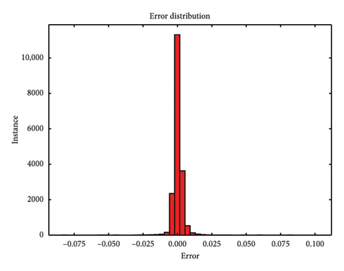
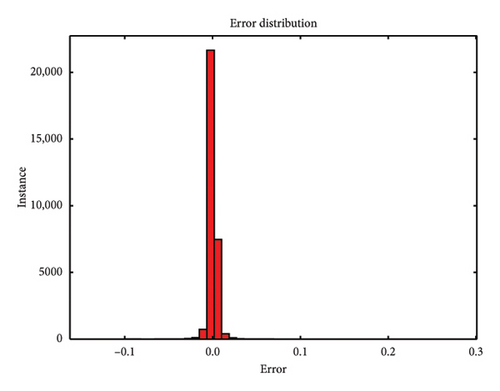
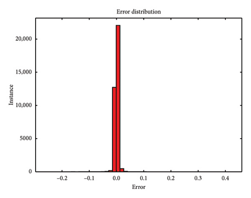
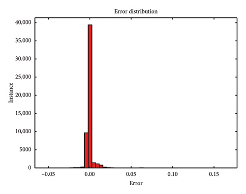
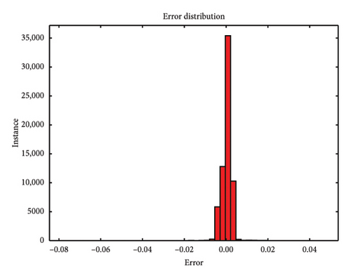
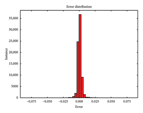
During the testing phase, error plots comparing predicted versus actual values for both single-element and multiple-element damage scenarios are depicted in Figure 10, respectively. Notably, even with a 5 dB S/N noise level, the errors predominantly cluster around zero, which underscores the model’s robustness and accuracy in identifying structural damage. Figures 10(a), 10(b), and 10(c) illustrate the error plots for the frame structure in the single-element damage case under different noise conditions: no noise, 3 dB S/N noise, and 5 dB S/N noise, respectively. Conversely, Figures 10(d), 10(e), and 10(f) display the error plots for the structure in the multiple-element damage case with no noise, 3 dB S/N noise, and 5 dB S/N noise, respectively.
4.3.5. Typical Damage Cases
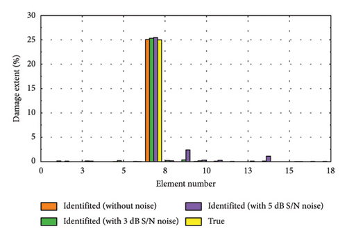
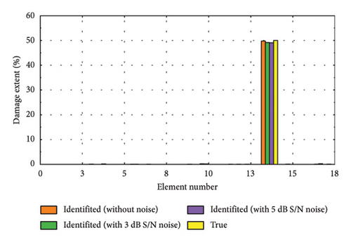
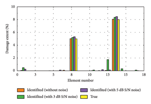
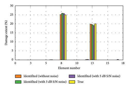
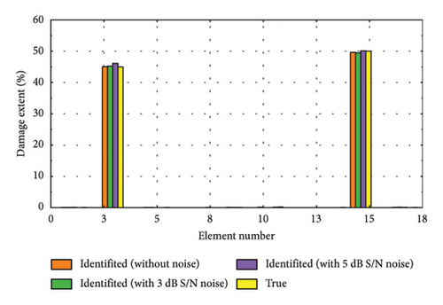
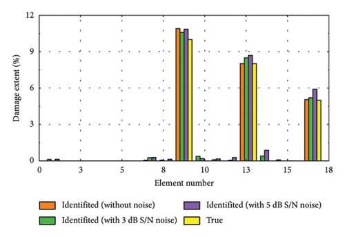
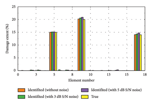
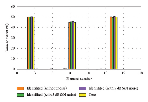
To further validate the efficacy of the proposed damage identification method, we randomly selected several representative damage samples from the test dataset and visualized the results, as depicted in Figure 11. It is evident that the identification accuracy is higher when no noise is added. However, despite some reduction in performance due to noise, the method remains capable of effectively pinpointing the location and assessing the severity of damage. Figures 11(a), 11(d), and 11(f) depict the identification results for minor damage, accurately detected by the method; Figures 11(b), 11(e), and 11(h) illustrate the results for moderate damage; and Figures 11(c), 11(g), and 11(i) show the results for severe damage.

4.4. Contrasting Raw Acceleration Signals
Conventional methods for structural damage identification primarily rely on the direct analysis of time-domain signals. This typically involves extracting statistical features from response signals or utilizing time-domain metrics to assess structural integrity. While intuitive, these approaches may lack sensitivity and accuracy, particularly when addressing complex or minor structural changes.
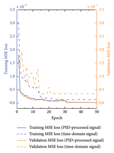
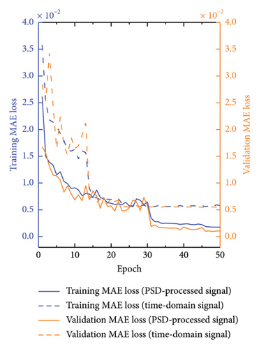
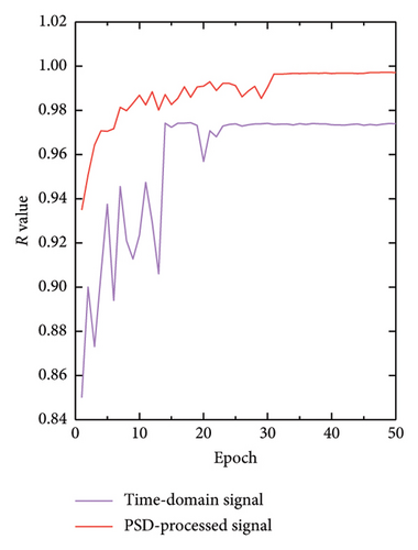
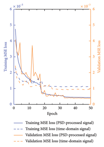
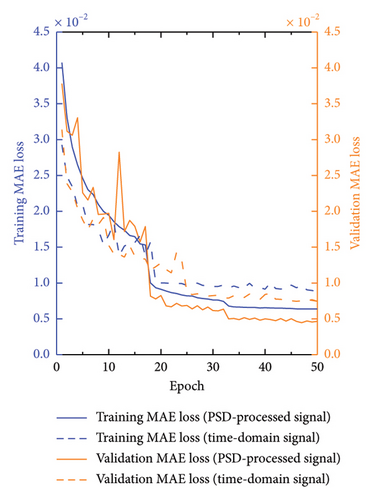
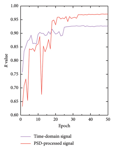
In this study, we trained the CNN by using time-domain acceleration signals and frequency-domain signals processed by PSD on the framework structure. For the time-domain acceleration signals, we utilized DenseNet with an input size of 60 × 4, maintaining consistent hyperparameter settings across the network as previously described. The comparative results of these training approaches are presented in Tables 1 and 2, where Table 1 shows the comparison without the addition of noise and Table 2 shows the comparison with the addition of 5 dB S/N noise. Our findings clearly demonstrate that the training effectiveness of frequency-domain signals, preprocessed by PSD, outperforms that of direct time-domain signals. This advantage holds true across scenarios with and without noise. These results suggest that PSD processing enhances signal characteristics, facilitating improved learning and identification of structural damage patterns by the neural network.
| Signal type | MSE loss | R value | MAE loss |
|---|---|---|---|
| PSD-processed signal | 2.2 × 10⁻⁵ | 0.991 | 1.0 × 10⁻³ |
| Time-domain signal | 3.0 × 10⁻⁴ | 0.97 | 5.2 × 10⁻³ |
| Signal type | MSE loss | R value | MAE loss |
|---|---|---|---|
| PSD-processed signal | 3.8 × 10⁻⁴ | 0.970 | 4.6 × 10⁻³ |
| Time-domain signal | 9.1 × 10⁻⁴ | 0.926 | 7.5 × 10⁻³ |
The analyses in Figures 12 and 13 illustrate the changes in the MSE, MAE, and Pearson’s correlation coefficient (R value), respectively, throughout the training process, with Figure 12 being the comparison without the addition of noise and Figure 13 being the comparison with the addition of 5 dB S/N noise. These metrics provide insights into the performance of the models trained on different types of signals: MSE, this figure compares the MSE for both time-domain and frequency-domain signals during the training process. The frequency-domain signals, processed by PSD, consistently show lower MSE values compared to time-domain signals. This indicates a smaller prediction error and a superior model fit for frequency-domain signals. MAE, this metric reflects the average deviation between the predicted and actual values. The frequency-domain signals exhibit lower MAE values, implying that their predictions are closer to the actual scenarios and therefore more accurate. R value, the R value for frequency-domain signal is generally higher than that for time-domain signals. This suggests that frequency-domain signals achieve better accuracy and reliability in model predictions, demonstrating a stronger linear correlation between predicted outputs and actual values. These findings underscore the efficacy of frequency-domain signals in structural health monitoring and highlight the crucial role of PSD preprocessing in enhancing the accuracy and efficiency of damage identification. By comparing the training performance of time-domain and frequency-domain signals, our study further confirms the significant advantages of utilizing frequency-domain analysis for structural assessments.
5. Experimental Validations
To experimentally validate the proposed method using transfer learning, a six-story framework structure is employed in this section to assess its generalization capability. The experimental models used in this validation have parameters identical to those of the numerical simulation model. This approach consists of fine-tuning a CNN model previously trained on numerical simulation data using a transfer learning technique. This process aims to enhance the model’s performance and adaptability to experimental data, thereby validating its effectiveness across different datasets and scenarios.
5.1. Data Generation
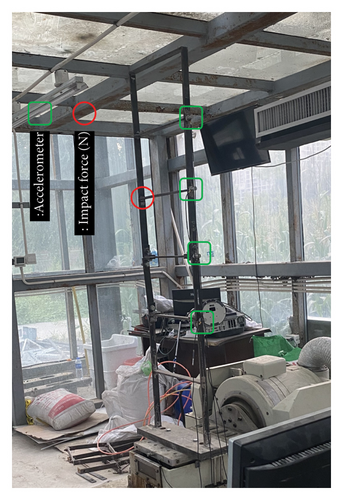
In this experiment, two elements were randomly selected for damage to retrain the CNN model, ensuring it learns actual structural features. For the frame structure, a damaged configuration with 25% damage to elements 3 and 9 was chosen as the training dataset for transfer learning. Similar to the numerical simulation approach, the reduction of the element cross-sectional area is employed to simulate structural damage. A random impact force of 90–110N was applied to node 9, with X-direction accelerations recorded from nodes 6, 8, 10, and 12 over 4 s, and the power spectrum difference was calculated. The retraining dataset consisted of 60 data points (20 per case) and split into thirds for training (70%), validation (15%), and testing (15%). Figure 14 illustrates the model of the frame structure: Figure 14(a) depicts the frame structure alongside its vibration device, while Figure 14(b) demonstrates the element with different cross-sectional areas.

5.2. Performance Evaluation
5.2.1. MSE
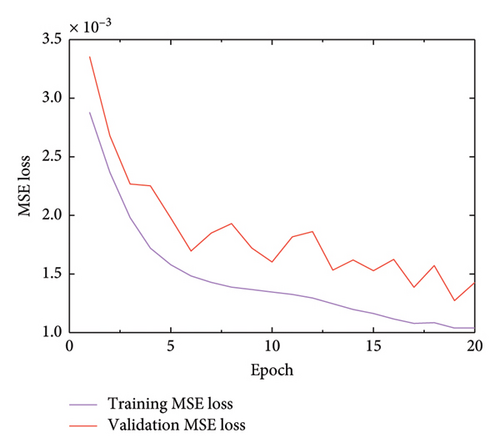
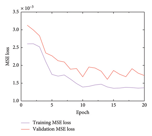
Initially, the MSE analysis depicted in Figure 15 reveals high values during the early stages of training. This discrepancy arises from mismatches between the experimental dataset (target domain) and the simulated dataset (source domain). However, after 20 rounds of training, a significant reduction in the MSE is observed, reaching as low as 1.3 × 10⁻³ for single-element damage in Figure 15(a) and 1.7 × 10⁻³ for multiple-element damage in Figure 15(b).
5.2.2. R Value
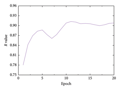
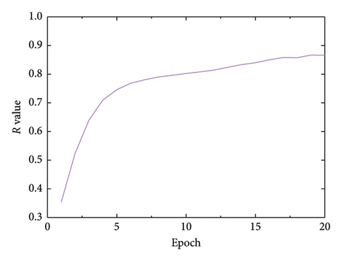
As illustrated in Figure 16, the initial R value at the beginning of the training phase is notably low, with values of 0.51 for single-element damage and 0.52 for multiple-element damage. These figures indicate a significant disparity between the experimental and simulated datasets. However, after 20 rounds of training, the CNN effectively adapted to the experimental data, resulting in a substantial increase in the R value to 0.91 for single-element damage and 0.88 for multiple-element damage.
5.2.3. Testing Phase
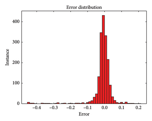
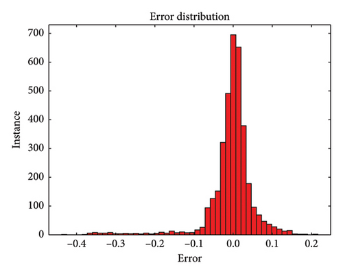
During the testing phase, error plots were used to assess the model’s performance on an unseen dataset. It is important to note that the test set in this study encompasses all potential damage scenarios in the frame structure, not limited to the specific 25% damage to elements 5 and 14 used in the transfer learning training detailed in Section 5.1. This evaluation is depicted in Figure 17, where Figure 17(a) illustrates single-element damage and Figure 17(b) shows multiple element damage.
5.2.4. Typical Damage Cases
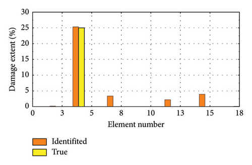
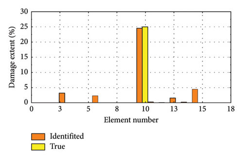
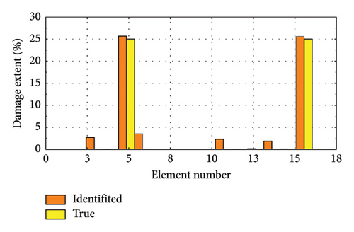
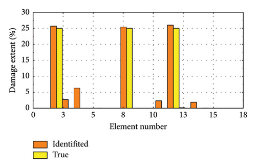
We selected several representative damage cases for visualization, as depicted in Figure 18. Figure 18(a) shows the scenario with 25% damage to element 4, while Figure 18(b) illustrates 25% damage to element 10. Figure 18(c) presents cases where both element 5 and element 16 are damaged by 25%, and Figure 18(d) depicts damage scenarios for element 6, element 8, and element 12, each with 25% damage.
6. Conclusion
This study presents an innovative approach to structural damage identification using a CNN in conjunction with PSD analysis of structural acceleration responses. The method involves converting CNN training data into a PSD matrix, enhancing the model’s precision in assessing structural damage. Leveraging transfer learning, the CNN is initially trained on simulated data and further fine-tuned using experimental data, thereby enhancing the robustness of real-world structural damage detection.
The proposed method’s validity was confirmed through simulations of a framework structure with added 3 dB S/N and 5 dB S/N noise, demonstrating robustness with Pearson’s correlation coefficient (R value) of 0.964 and an MSE loss of 4.6 × 10⁻⁴ under 5 dB S/N noise. Additionally, the CNN model’s performance was evaluated using both time-domain signals and PSD-processed signals, highlighting superior accuracy of PSD-processed signals compared to time-domain signals, particularly in noisy conditions. In experimental validations, the CNN model undergoes fine-tuning via transfer learning with a limited set of experimental data. This approach achieves a R value of 0.90 and an MSE loss of 1.7 × 10⁻³, further validating its applicability across actual structures.
However, this method faces certain challenges, particularly the computational intensity of processing frequency domain signals. More importantly, real-world structures are likely to experience a variety of complex damage scenarios beyond simple reductions in stiffness. Addressing these real-life damage conditions will be a primary focus of our future research. At the same time, optimizing the computational efficiency of frequency domain signal processing remains a critical area for improvement.
Conflicts of Interest
The authors declare no conflicts of interest.
Funding
This research did not receive any specific funding from public, commercial, or not-for-profit organizations.
Open Research
Data Availability Statement
The data that support the findings of this study are available from the corresponding author upon reasonable request.


