Structural Control and Health Monitoring

Volume 2025, Issue 1 4714219

Research Article

Open Access

Stochastic Static Model Updating of Bridge Using Homotopy Method and Pre-Estimated Solution Domain

Bin Huang,

Bin Huang

orcid.org/0000-0003-3454-6952

School of Civil Engineering and Architecture , Wuhan University of Technology , Wuhan , 430070 , China , whut.edu.cn

Search for more papers by this author

Kaiyi Xue,

Kaiyi Xue

orcid.org/0009-0004-4086-3553

School of Civil Engineering and Architecture , Wuhan University of Technology , Wuhan , 430070 , China , whut.edu.cn

Search for more papers by this author

Hui Chen,

Corresponding Author

Hui Chen

[email protected]

orcid.org/0000-0003-1258-021X

School of Civil Engineering and Architecture , Wuhan University of Technology , Wuhan , 430070 , China , whut.edu.cn

College of Post and Telecommunication , Wuhan Institute of Technology , Wuhan , 430073 , China , wit.edu.cn

Search for more papers by this author

Ming Sun,

Ming Sun

School of Civil Engineering and Architecture , Wuhan University of Technology , Wuhan , 430070 , China , whut.edu.cn

Department of Mechanical & Aerospace Engineering , University of Strathclyde , Glasgow , G1 1XQ , UK , strath.ac.uk

Search for more papers by this author

Zhifeng Wu,

Zhifeng Wu

orcid.org/0000-0003-2707-6171

School of Civil Engineering and Architecture , Wuhan University of Technology , Wuhan , 430070 , China , whut.edu.cn

School of Civil and Hydraulic Engineering , Huazhong University of Science and Technology , Wuhan , 430074 , China , hust.edu.cn

Search for more papers by this author

Bin Huang,

Bin Huang

orcid.org/0000-0003-3454-6952

School of Civil Engineering and Architecture , Wuhan University of Technology , Wuhan , 430070 , China , whut.edu.cn

Search for more papers by this author

Kaiyi Xue,

Kaiyi Xue

orcid.org/0009-0004-4086-3553

School of Civil Engineering and Architecture , Wuhan University of Technology , Wuhan , 430070 , China , whut.edu.cn

Search for more papers by this author

Hui Chen,

Corresponding Author

Hui Chen

[email protected]

orcid.org/0000-0003-1258-021X

School of Civil Engineering and Architecture , Wuhan University of Technology , Wuhan , 430070 , China , whut.edu.cn

College of Post and Telecommunication , Wuhan Institute of Technology , Wuhan , 430073 , China , wit.edu.cn

Search for more papers by this author

Ming Sun,

Ming Sun

School of Civil Engineering and Architecture , Wuhan University of Technology , Wuhan , 430070 , China , whut.edu.cn

Department of Mechanical & Aerospace Engineering , University of Strathclyde , Glasgow , G1 1XQ , UK , strath.ac.uk

Search for more papers by this author

Zhifeng Wu,

Zhifeng Wu

orcid.org/0000-0003-2707-6171

School of Civil Engineering and Architecture , Wuhan University of Technology , Wuhan , 430070 , China , whut.edu.cn

School of Civil and Hydraulic Engineering , Huazhong University of Science and Technology , Wuhan , 430074 , China , hust.edu.cn

Search for more papers by this author

First published: 01 March 2025

https://doi.org/10.1155/stc/4714219

Academic Editor: Ka-Veng Yuen

Share a link

Email
Wechat
Bluesky

Abstract

When implementing structural model updating, whether the model is stochastic or deterministic, the ill-posed issue is a challenging problem. To effectively address this problem, this paper proposes a new static stochastic model updating method, which combines the homotopy method with the pre-estimation technique of solution domains of the updating quantities. Firstly, considering the uncertain static measurement displacements, the solution domains of updating factors in structural models such as bridges are derived in terms of the sensitivity of static strain energy. Then the homotopy method is used to transfer the stochastic static model updating equation into a series of deterministic recursive equations about the expansion coefficients of updating factors. Within the pre-estimated solution domains, the expansion coefficients of the updating factors can be solved by the L-curve method and the convex optimization. When the measurement positions do not contain the loading points, a model expansion strategy is provided. Two numerical examples demonstrate that the proposed method can offer stable updating results, which coincide very well with those assumed real values, in the cases of high-dimension and limited measurement points. And when the displacements at the loading points are not directly measured, compared with the Bayesian method with the finite element samples, the proposed method has higher computational efficiency with the equivalent accuracy. When updating a practical continuous box-girder bridge, the proposed method can efficiently update a large finite element model, and the statistics of updating results agree very well with those of the static measurement data.

1. Introduction

The initial finite element (FE) model of a bridge structure is typically established based on engineering design drawings. However, during the construction process, many factors, such as the concrete maintenance condition, construction technology, material discreteness, and external environment, can lead to the difference between the actual structure and the initial FE model. After a period of use, due to material degradation and other reasons, this difference may further amplify, causing the initial FE model to fail to accurately match with the true structure. Therefore, measurement responses are needed to update the structural initial model [1, 2], ensuring that the updated model can be employed to accurately predict the dynamic and static characteristics of the true structure and provide the reference model for the condition assessment of the structure.

The response indicators often used in the FE model updating include dynamic and static ones. The dynamic indicators, such as the frequencies, modal shapes, and frequency response functions, have attracted widespread attention [3–6]. On the other hand, the model updating methods utilizing the static indicators such as deflections have also been favored by scholars [7–9]. Particularly, for bridge structures, the static load test is one of the important tasks specified in their inspection standards [10]. In general, the static indicators are independent of the structural mass and damping ratio, which is beneficial for updating structural FE models [11] or identifying stiffness parameters [12]. In recent years, with the rapid advancement of vision-based and AI-enabled measurement technologies [13–15], the utilization of static measurement data has become increasingly common.

Being influenced by the environment, testing persons, and testing instruments, the static measurement data inherently possess uncertainties [16]. When the uncertain static measurement data are used for the FE model updating, the inferred structural parameters also exhibit statistical characteristics. Hence, the static FE model updating that relies on uncertain measurement data will be a main development [17], and the related methods are referred to as the stochastic static model updating methods.

The stochastic static model updating methods, similar to the dynamic ones, mainly include the Monte Carlo simulation (MCS) [18, 19], perturbation method [20, 21], Bayesian method [22–27], hybrid perturbation-Galerkin stochastic model updating method [28], and homotopy stochastic model updating method [29, 30]. Due to the long calculation time when dealing with large structures, the MCS method is limited in engineering applications [19]. Although the perturbation method has high computational efficiency, it is not suitable for handling the engineering problems with the parameters of large variation [21]. The Bayesian methods transform inverse problems into forward problems, effectively overcoming the nonuniqueness issue [22, 23]. Jia et al. [24, 25] utilized the long-term monitored static deflections and the Markov Chain Monte Carlo (MCMC) methods to infer the critical parameters, such as the stiffness, creep, shrinkage, prestress level, and dead load level, of a prestressed concrete bridge. Although the Bayesian methods are effective in the uncertain estimation of low-dimensional parameters, they are also affected by the accuracy of prior information [26] and difficult to converge when facing high-dimensional parameters [27]. Different from the Bayesian methods, based on the model updating frame about stochastic FEs, Huang et al. [28] and Wu et al. [29] have recently proposed the hybrid perturbation-Galerkin stochastic model updating method and the homotopy stochastic model updating method, respectively. Both the methods aim to establish the stochastic model updating equations and utilize the stochastic perturbation-Galerkin method or the stochastic homotopy method to solve them. The main features of such type of methods include the highly computational efficiency and the capability of dealing with the large fluctuation of the stochastic updating parameters with arbitrary probability distributions. However, similar to many early deterministic FE model updating methods [30–33], these methods also encountered the ill-posed issue when solving inverse problems. These challenges highlight the need for robust solutions to tackle the ill-posedness in these FE model updating equations.

One of the primary methods for coping with the ill-posed problem in solving FE model updating equations is the regularization method [34, 35]. The main idea of regularization is to ensure the existence and uniqueness of the solution by introducing additional assumptions such as regularization parameters. The key point is to determine the optimal regularization parameter. For example, to obtain the regression coefficients of a standard linear regression model, an optimal regularization parameter is determined by maximizing the marginal likelihood about the regression coefficients [36]. When using the Tikhonov regularization to realize the Bayesian estimation of subsurface fault slips, Ortega et al. [37] used the target posterior variance of the estimated slip model as a regularization parameter. Renaut et al. [38] used the Golub–Kahan iterative bidiagonalization of the regularized problem to decide the regularization parameter so that the Tikhonov regularized least squares functional satisfies a χ² distribution. Xie et al. [39] proposed an efficient Laplace prior-based sparse Bayesian learning for the structural damage identification and realized the maximum likelihood estimation of the regularization parameter. Unfortunately, up to date, there is still no unified standard for determining the optimal regularization parameter [40].

Another approach for handling this ill-posed problem is to control the range of the solution domain. To promise the smoothness of the predicted data in geophysical inverse problems, Gholami and Siahkoohi [41] added an additional penalty term to the classical Tikhonov regularization, and the penalty term actually is a constraint or potential function about the solution. Gülcehre and Bengio [42] emphasized the importance of prior information on the optimization in the process of exploring the effect of prior knowledge into the intermediate level of deep supervised neural networks. However, so far, there are few reports on the estimation of solution domains for stochastic FE model updating problems.

To solve the ill-posed problem in updating stochastic FE models, this paper proposes a new stochastic static model updating method based on the homotopy method and the pre-estimation of solution domains of updating factors. Using the uncertain measurement data, this new method is then employed to update the FE model of bridge. At first, utilizing the measured static displacements, the solution domains of updating factors in a bridge structure are pre-estimated in terms of the sensitivity of static strain energy. Afterward, the homotopy method is used to transfer the stochastic static model updating equation into a series of deterministic recursive equations about the expansion coefficients of the updating factors. Within the pre-estimated solution domains, the expansion coefficients of the updating factors can be determined by the L-curve method and the convex optimization, and the ill-posed problem is effectively avoided. During the updating process, if the measurement positions do not contain the loading points, a model expansion strategy is provided to decide the displacements at those loading points. Two numerical examples demonstrate that because of the usage of the pre-estimated solution domains, the proposed method can offer stable and accurate updating results, which coincide very well with those assumed real values, in the case of high-dimension and limited measurement points. And when the displacements at the loading points are not directly measured, compared with the Bayesian method with the FE samples, the proposed method has higher computational efficiency with the equivalent accuracy. When updating a practical continuous box-girder bridge, the proposed method can efficiently update a large FE model, and the statistics of updating results are consistent with those of the measured static data.

The organization of the paper is as follows. Section 2 derives the pre-estimated solution domain using the concept of strain energy sensitivity, builds up the homotopy stochastic model updating equation, and solves the updating equations by the L-curve method with the pre-estimated solution domain and the convex optimization. Sections 3 and 4 use a numerical example to illustrate the proposed method, respectively. Section 5 discusses the application of the proposed method on a practical box-girder bridge. Finally, the conclusions are drawn.

2. Theoretical Frameworks

2.1. Pre-Estimation of Solution Domains of Updating Factors

Consider a bridge structure subjected to static loads. Assuming that the bridge structure has N degrees of freedom (DOF), the static equilibrium equation for the structure can be expressed as

()

where K₀ represents the stiffness matrix with dimensions N × N in the initial FE model of the structure. F is a N × 1 dimensional static load vector. V₀ denotes the displacement vector.

For the practical bridge structure, the actual stiffness matrix K_d can be written as

()

where ΔK represents the variation of the initial stiffness matrix. Assuming that a bridge structural system has n elements, ΔK can be further expressed as the sum of the expanded element stiffness matrices K_i multiplied by the updating factors β_0i, which is

. β_0i represents the rate of change of the physical parameter such as the elastic modulus in the ith element.

Considering that the load in the static equilibrium equation in equation (1) is the same as the load experienced by the actual structure, there is

()

where V_d is the displacement vector of the actual structure under the load vector F.

Substituting equations (2) into (3), one can obtain

()

The first-order Taylor expansion of V_d in equation (4) can be written as

()

Then using (5), (4) can be further written as

()

where

can be neglected since only the first-order terms about β_0i are considered. So the first-order sensitivity of the displacement vector V_d with respect to the updating factors β_0i can be obtained as

()

When subjected to a static load, the structure will store the strain energy. The static strain energy in each element is named the static strain energy index, which is sensitive to the variation of the structural parameter in each element [43]. Here the static strain energy index sse_j of the jth element in the structural initial model can be formulated as

()

Similarly, the static strain energy index

of the jth element of the actual structure is represented as

()

where K_dj denotes the expanded element stiffness matrix of the jth element in the actual structure. The difference between the static strain energy indexes of the initial model and the actual structure is expressed as

()

Additionally, the first-order Taylor expansion of the static strain energy variation Δsse_j of the jth element about β_0j can be represented as

()

where Δsse_j(0) is zero. Simultaneously, considering equations (10) and (11), one can obtain

()

Since V₀ does not contain the parameter β_0j, equation (12) is rewritten as

()

Further there is

()

Substituting (7) into (14), we have

()

Taking equation (2) into account, one can have

. Then an alternative expression for Δsse_j in equation (10) can be represented as

()

When the variation of structural parameters is small, it is assumed that K_dj can be replaced by the initial stiffness matrix K_j of the jth element in equation (16). Letting the right side of equation (15) equal to that of equation (16) leads to

()

Upon further transformation, an approximation of the jth updating factor β_0j can be obtained as

()

Furthermore, considering the uncertainty in the measured static displacements of the structure, it is assumed that the mean value of the displacement vector V_d is V_d0, and the vector, whose element is the standard deviation (SD) of the corresponding element of the vector V_d, is denoted as σ_d. Under normal circumstances, it can be roughly assumed that the SDs of the measured displacements and the updating factors are linearly related [44]. Furthermore, the three-sigma rule in normal distributions is used to represent the range of the measured displacements, corresponding to over 88.8% of the entire range of non-normal distributions. Therefore, the lower bound

and the upper bound

of the jth updating factor β_0j are represented, respectively, as

()

Then the lower and upper bound vectors of the updating factors can be represented by the two vectors and . Since the lower and upper bound vectors, Γ^down and Γ^up, of the updating factors cover relatively large ranges, the real updating factor vector generally falls within these ranges. In this paper, we name these ranges as the pre-estimated solution domains for the updating factors in the model updating.

2.2. Homotopy Approach for the Updating Factors

When employing static displacements to update the FE model of a bridge structure, according to equation (4), the deterministic static model updating equation is formulated as

()

Furthermore, when considering the uncertainty of measurement displacements, the static measurement displacement vector can be expressed as

()

where η_tV_d1 denotes the uncertain part of the measurement vector. t indicates the serial number of measurement point, and l denotes the total number of measurement points. η_t denotes the stochastic variable of the tth measurement displacement. It is assumed that the stochastic displacements at different measurement points are fully related, so there is η_t = η. Substituting (22) into (21), the deterministic model updating equation in equation (21) can be transformed into a stochastic model updating equation, as

()

where β_i(η), i = 1, 2, ⋯, n, become the stochastic updating factors. Equation (23) can be further written as the matrix form as

()

where C₀ = [K₁V_d0, K₂V_d0, …, K_nV_d0], C₁ = [K₁V_d1, K₂V_d1, …, K_nV_d1],

, R₀ = K₀V_d0, and R₁ = K₀V_d1.

To build up a homotopy relation between the deterministic updating factor vector β₀, whose elements are β_0i (i = 1, 2, …, n), and the stochastic updating vector β(η), equation (24) is constructed as the zero-order deformation equation, as

()

where w is the embedding parameter varying between 0 and 1 and h is an auxiliary parameter. Ξ(η, h, w) is the homotopy construction related to the stochastic updating factor β, which is also the function of η, h, and w. It is important to note that the vector β₀ is treated as the initial approximation of the stochastic vector function Ξ(η, h, w), which can be obtained by solving equation (24) when η = 0.

From equation (25), it can be observed that when w = 0, Ξ(η, h, 0) = β₀, and when w = 1, there exists Ξ(η, h, 1) = β(η). The function Ξ(η, h, w) can be expressed as a Maclaurin series, as

()

In equation (26), Ξ^[m](η, h, 0) represents the mth order partial derivative of Ξ(η, h, w) with respect to w when w = 0.

Calculating the partial derivative of the zeroth-order deformation equation in equation (25) with respect to w, the first-order deformation equation can be achieved as

()

where the symbol Ξ denotes Ξ(η, h, w). When w = 0, equation (27) will become

()

Moreover, considering that C₀β₀ − K₀V₀ + R₀ = 0, equation (28) further generates

()

where β₁ is determined by the following equation, which is

()

Taking the partial derivative of equation (27) with respect to w, the second-order deformation equation is yielded, as

()

When w = 0, equation (31) is simplified as

()

where β₂ is obtained by the following equation, as

()

Following the above steps, we can determine the mth order partial derivative of Ξ(η, h, w) about w when w = 0. Then assuming that w = 1, the homotopy series solution in equation (25) or the stochastic updating factor vector β can be expressed as

()

where ξ_m,k(h), k = 1, 2, …, m, is the deterministic function, which can be represented as

()

The value of the homotopy coefficient h in equation (35) can be determined through the probability residual error minimization method outlined by reference [44].

2.3. Solutions of Recursive Equations Using the L-Curve Method and Convex Optimization

When solving the recursive equations about Ξ^[i](i = 1, 2, …, m), one of the most effective solution methods is the Tikhonov regularization. However, it is found that about the traditional regularization methods, the selection of the regularization parameter depends on the experience, which often results in the instability of the solutions [29, 45]. Although some new methods like the iterative regularization method are applied to automatically determine the solution, the solution often converges slowly and easily falls into a local optimization status [46, 47]. To address this problem, this paper combines the pre-estimated solution domains with the L-curve regularization method as well as the convex optimization method to solve the coefficient vectors β_j in equation (34), which greatly improves the accuracy of the regularization and effectively avoids the ill-posed problem.

To solve the vector β₀ in equation (25), the optimal objective function about the vector β₀ is expressed as

()

where

represents the 2-norm and α₀ is the regularization parameter.

Firstly, the regularization method α₀ in equation (36) is achieved by the L-curve regularization method. Then considering the pre-estimated solution domain of the vector β₀ as determined in Section 2.1, the constraint of the objective function in equation (36) can be described as

()

Further the convex optimization method [48] is used to optimize the objective function in equation (36) subjected to the constraint in equation (37) so as to obtain the vector β₀. Note that although the parameter α₀ achieved by the L-curve regularization method may be not good enough, the final optimal result about the vector β₀ is very accurate with the aid of the pre-estimated solution domain.

Afterward, the optimal objective functions about the vectors β_j are represented as

()

Using the traditional regularization methods to optimize the functions in equation (38), the vectors β_j can be achieved. It is worth mentioning that the accuracy of the vectors β_j should be high since it depends on the accuracy of the vector β₀.

Following the above steps, the coefficient vectors β_j of the stochastic updating factor vector β in equation (34) can be recursively solved.

2.4. Expansion of Measurement Displacement Vector

When constructing the stochastic model updating equations, it is necessary to match the structural stiffness matrix with the number of measured DOFs, which correspond to the measurement points and loading points. Utilizing the Guyan reduction method, the condensed form of the initial stiffness matrix K₀ can be obtained as

()

where K_0d represents the condensed stiffness matrix. K_0aa, K_0ab, K_0bb, and K_0ba denote the submatrices of the initial structural stiffness matrix K₀ associated with the measurement DOFs, the nonmeasurement DOFs, or the mix of them, respectively. The subscripts a and b indicate the measurement and the nonmeasurement DOFs, respectively. Employing the method outlined in the reference (Wu et al. [29]), the condensed expansion stiffness matrix of the jth element can be obtained as

()

where, K_jaa, K_jab, K_jbb, and K_jba represent the submatrices, which are associated with the measurement DOFs, the nonmeasurement DOFs, or the mix of them, of the initial expansion stiffness matrix K_j of the jth element, respectively.

Generally, the measurement points do not contain the loading points, where the dimension of the measured displacements is less than the dimension of K_0d. In order to match the DOF number of the measured displacements with that of the condensed stiffness matrix K_0d, an extension of the measured displacements is required. The equilibrium equation in equation (1) can be condensed as

()

where

denotes the extended measurement displacement vector matched with K_0d. F_a represents the load vector related to the DOFs at all measurement and loading points.

Transferring equation (41) into a partitioned matrix form, there is

()

where K_dmm, K_dms, K_dsm, and K_dss are the submatrices of the matrix K_0d and the subscripts m and s denote the measurement and loading points, respectively.

and F_am denote the displacement and load vectors at the measurement points, respectively.

and F_as denote the displacement and load vectors at the loading points, respectively.

represents the displacement vector to be extended, corresponding to the loading points.

From equation (42), the displacement vector

at the loading points can be represented as

()

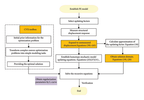
Up to now, all elements of the vector are known. Then the matrix K₀ and the vector V_d in the recursive equations (21), (22), and (23) are replaced by K_0d and , respectively. In this way, even if the measurement points do not contain the loading points, the proposed updating method is also available. When is uncertain, it can be divided into the deterministic and stochastic parts so that equation (43) can be used to decide the stochastic vector. For simplicity, the new stochastic static model updating method based on the homotopy method and the pre-estimated solution domains is denoted as HSMI, and the flowchart of the new method is illustrated in Figure 1.

Details are in the caption following the image — **Figure 1**
Open in figure viewer PowerPoint

Flowchart of the proposed method.

3. Numerical Example I: One Single Story Frame

Consider a single-story frame characterized by the uniform rectangular cross section, whose size is 0.15 by 0.2 m, as shown in Figure 2. The FE model of the frame is composed of 24 two-dimensional beam elements and 25 nodes. Each node is endowed with three DOFs, which include the horizontal displacement, vertical displacement, and rotation. The length of the elements 1 to 8 and 17 to 24 is 0.2 m, and that of the elements 9 to 16 is 0.3 m. The elastic modulus is 2.8 × 10¹⁰Pa.

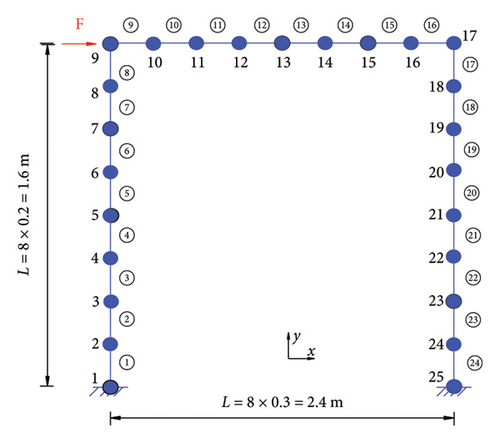
It is assumed that the elastic modulus of each element changes. For the ith element, the updating factor α_i is defined as the ratio of variation of the real elastic modulus relative to the initial one, and the preset values of all updating factors are listed in Table 1.

Table 1. The preset values of updating factors.

Factor	α₁	α₂	α₃	α₄	α₅	α₆	α₇	α₈	α₉	α₁₀	α₁₁	α₁₂
Value	−0.30	−0.20	−0.40	−0.30	−0.30	−0.30	−0.35	−0.30	−0.30	−0.20	−0.25	−0.30

Factor	α₁₃	α₁₄	α₁₅	α₁₆	α₁₇	α₁₈	α₁₉	α₂₀	α₂₁	α₂₂	α₂₃	α₂₄

Value	−0.40	−0.30	−0.25	−0.25	−0.30	−0.25	−0.20	−0.35	−0.30	−0.40	−0.20	−0.10

At node 9 of the frame, a load of 10 kN is applied in the horizontal direction. Two cases are considered. In Case I, all horizontal displacements at the nodes of the two columns and the vertical displacement at the nodes 10 to 16 are measured. Case II does not consider the horizontal displacements of nodes 2, 5, 8, 18, 21, and 24 and the vertical displacement at node 13. All measured nodal displacements are supposed as random and follow the beta distributions with the coefficient of variation (COV) ranging from 0.04 to 0.06. The initial values and statistical measurement values of the nodal displacements in the two cases are presented in Table 2.

Table 2. Initial displacements and statistical measurement displacements of all nodes (×10⁻³ m).

Node	2	3	4	5	6	7	8	9	10	11	12	13
Initial	0.032	0.119	0.246	0.399	0.564	0.726	0.871	0.985	−0.087	−0.102	−0.066	−0.003
Mean	0.044	0.159	0.331	0.541	0.767	0.988	1.183	1.333	−0.107	−0.119	−0.067	0.020
COV	0.058	0.056	0.042	0.045	0.047	0.054	0.043	0.054	0.042	0.053	0.050	0.056
Case I	H	H	H	H	H	H	H	H	V	V	V	V
Case II	N	H	H	N	H	H	N	H	V	V	V	N

Node	14	15	16	17	18	19	20	21	22	23	24

Initial	0.060	0.098	0.085	0.971	0.859	0.717	0.557	0.394	0.243	0.118	0.032
Mean	0.104	0.149	0.122	1.312	1.155	0.955	0.732	0.508	0.303	0.140	0.037
COV	0.054	0.058	0.058	0.047	0.054	0.044	0.041	0.055	0.050	0.050	0.058
Case I	V	V	V	H	H	H	H	H	H	H	H
Case II	V	V	V	H	N	H	H	N	H	H	N

Note: V, H, and N denote the vertical displacement measured, the horizontal displacement measured, and no measurement, respectively.

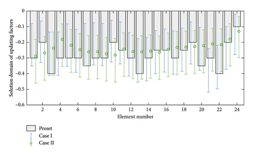
Firstly, using the means of the measurement displacements shown in Table 1, the lower and upper bounds, Γ^down and Γ^up, of the solution domains of all deterministic updating factors β_0i (i = 1, 2, …, n) are computed by employing equations (19) and (20) and are depicted in Figure 3. From Figure 3, it is clearly observed that the solution domain pre-estimated by the static strain energy index method completely covers the preset values of the updating factors in the two cases. Even if the number of measurement displacements is reduced one-thirds, the preset values are still in the pre-estimated solution domains.

Next, the three methods, which include the proposed HSMI method, the proposed method without using the pre-estimated solution domains, referred to as HSMN, and the MCS method with 1 × 10⁵ samples, are used to calculate the statistics of the updating factors. Figures 4 and 5 present the means and SDs of the updating factors in Case I and Case II, respectively. From Figure 4, it is observed that the means and SDs of the updating factors obtained from the proposed HSMI method closely match with the results from MCS. However, the SDs of the factors from the HSMN method without the pre-estimated solution domains significantly deviate from those of MCS, and the maximum deviation amplitude reaches 40% that of MCS.

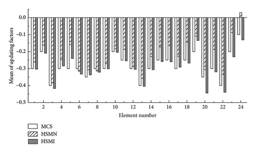
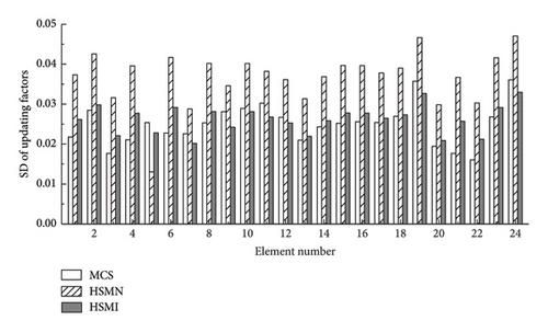
Figure 5 shows the statistical updating results in Case II. From Figure 5, it is watched that the means and SDs of the updating factors from the proposed HSMI method slightly deviate from those from MCS, where the maximum deviation amplitudes of the mean and SD are within 10% and 5% those of MCS, respectively. This result indicates that even if the number of measurement points is 16 or the two-thirds of the original one, the updating results of the proposed method are still very well. However, the statistical updating results from the HSMN method without the pre-estimated solution domains have a large deviation from those of MCS. And the means of the updating factors in the elements 5 and 20 are wrongly updated. The maximum deviation amplitude of the SD surpasses 50% that of MCS. This result demonstrates that the pre-estimated solution strategy in the proposed method effectively addresses the ill-posed problem of the updating equations caused by the reduction in measurement points.

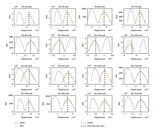
Finally, the stochastic updating factors obtained in Case II were utilized to determine the probability density functions (PDFs) of displacements at the measurement points and are depicted in Figure 6. It is found from Figure 6 that the PDF curves of structural displacements obtained from the proposed method closely align with the PDF curves of measurement displacements. In contrast, the HSMN method fails to produce the PDF curves matching with those of MCS. These results further illustrate that after using the pre-estimated solution domains of the deterministic updating factors β_0i, the proposed method can effectively and correctly update the structural FE model even if the number of measurement points is less than that of updating factors.

4. Numerical Example II: A Curved Bridge With Single Box and Single Cell

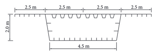
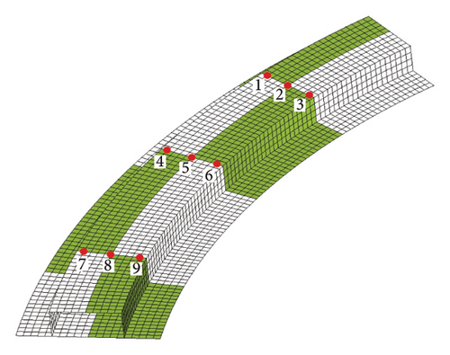
Consider a single-box single-cell curved steel bridge with both ends simply supported, as shown in Figure 7. The height of the box girder is 2 m, the radius of curvature is 50 m, the curvature angle is 45^o, and the length is 39.27 m. The thickness of the plate is 0.02 m. The U-shaped stiffeners have a thickness of 0.008 m. The elastic modulus Ε = 2.05 × 10¹¹Pa, and Poisson’s ratio v = 0.3. The FE model, which is shown in Figure 7(b), of the bridge is established using the ANSYS software, where the SHELL181 element is employed to simulate the plate. The entire bridge is divided into 3306 elements, and each element has 4 nodes. Each node has three translational DOFs and three rotational DOFs, resulting in a total of 20,064 DOFs for the bridge.

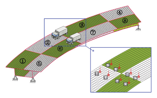
The box-girder bridge is divided into 8 regions as shown in Figure 7(b), and each region shares a common elastic modulus. It is assumed that the elastic modulus of each region has a certain level of degradation, and the percentage of degradation is defined as the updating factor whose value is listed in Table 3.

Table 3. The value of the updating factor of each region.

Updating factor	θ₁	θ₂	θ₃	θ₄	θ₅	θ₆	θ₇	θ₈
Value	−15%	−30%	−10%	−10%	−15%	−30%	−10%	−15%

As shown in Figure 7(b), two trucks are applied for loading on the bridge. Each vehicle is 1.8 m wide and 3 m long. The weight of single vehicle is 60 kN, with 10 kN on each front wheel and 20 kN on each rear wheel. The eight loading points correspond to nodes 10 to 17 in the FE model. Vertical displacements at 9 points at the bridge bottom are selected as the mean of the measured displacements, as shown in Figure 8. To simulate the random measurement results, after obtaining the vertical displacements or the real displacements at the measurement points of the FE model with the degraded elastic modulus, the values of the vertical displacements through adding the random errors of 5% normal distributions are assumed as the mean values of the measured displacements. Meanwhile, the COV values of the measurement displacements range from 0.04 to 0.06. And it is assumed that the measurement displacements obey the normal distributions. The statistics of the measurement displacements are shown in Table 4.

Table 4. The statistics of the measurement displacements (mm).

Measurement point	1	2	3	4	5	6	7	8	9
Initial displacement	−5.597	−5.038	−4.505	−8.544	−7.768	−7.050	−4.536	−3.610	−4.063
Measurement displacement (mean)	−5.880	−5.308	−4.759	−8.944	−8.128	−7.440	−4.757	−3.815	−4.278
Measurement displacement (COV)	0.049	0.048	0.049	0.055	0.046	0.056	0.049	0.041	0.044

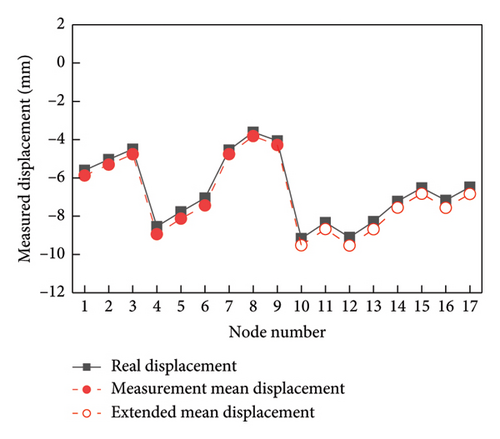
Firstly, the measurement vertical displacements at nodes 1 to 9 are employed to obtain the extended measurement displacements at nodes 10 to 17. It is crucial to note that the SDs of displacements at nodes 10 to 17 are also required. After extending the measured displacements, the means of the measurement displacements at nodes 1 to 17 are drawn in Figure 9. It is seen from Figure 9 that like the mean values of the assumed measurement displacements at the measurement points, the means of the extended measurement displacements are also close to the real displacements, where the small deviations come from the transmission of measurement errors.

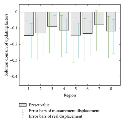
Based on the uncertain measurement displacements after being extended at nodes 1 to 17, the solution domains of the eight updating factors can be estimated and are depicted in Figure 10. For comparison, the solution domains of the updating factors determined by the real displacements are also presented. It can be observed from Figure 10 that the ranges of the solution domains obtained by the measured displacements contain those obtained by the real displacements. Moreover, the solution domains of the deterministic updating factors β_0i calculated by the proposed method cover or approach the predefined 8 updating factors in Table 3. These results demonstrate that although the measurement displacements have an uncertain measurement error, the solution domains of the updating factors β_0i pre-estimated by the proposed method still can contain or be near to the assumed values of the updating factors.

Afterward, the proposed HSMI method, the Bayesian method with Delayed Rejection Adaptive Metropolis sampling, and the MCS method, where the number of samples is 1 × 10⁵, are used to calculate the means and SDs of the updating factors. About the Bayesian method, the likelihood function used is

()

where y_k represents the measurement or observation result at the kth time and

denotes the number of observations. y_cal represents the structural response calculated by the identified structural parameters. C_y is the covariance matrix of the observation responses.

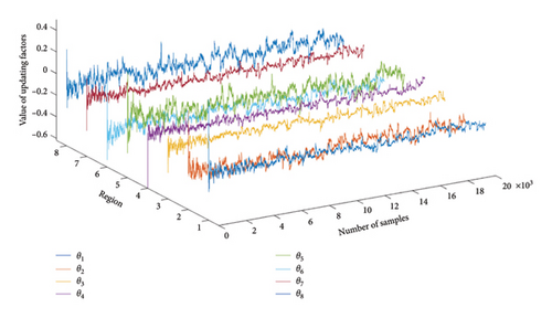
Once the likelihood function in equation (44) is known, the posterior PDF of the updating factors can be obtained using the MCMC sampling method as employed in reference [4]. The measured displacement responses are the same as those used in the proposed HSMI method. The number of rejections is set to 2 in the MCMC sampling. In each iteration of the Bayesian method, the FE samples are calculated, and the total number of samples is 20,000. Through using the Bayesian updating method, the Markov chains of the updating factors obtained are drawn in Figure 11. It can be observed from Figure 11 that after 5000 samples, the Markov chains of all updating factors begin to converge.

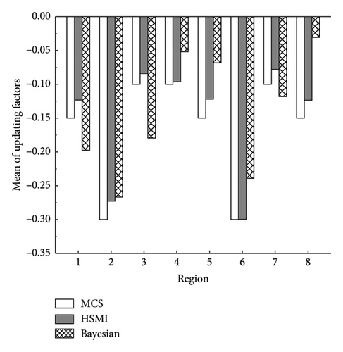
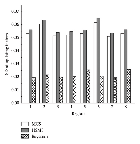
By discarding the initial 5000 samples, the remaining 15,000 samples are kept to calculate the means and SDs of the updating factors and are plotted in Figure 12 together with the results from the proposed HSMI method and MCS. From Figure 12, it can be observed that the means obtained from the proposed method and the Bayesian method approach the results of the MCS method. The SD values of the updating factors by the proposed method agree with those of MCS very well. The SDs of updating factors from the Bayesian method are significantly less than the results of MCS, which may be due to the relatively large SD of the measurement displacements.

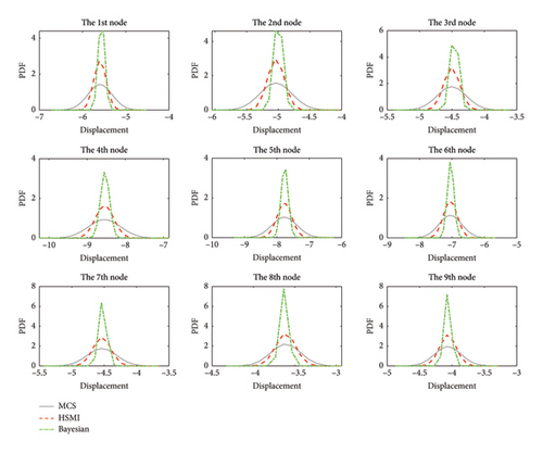
On the basis of the stochastic updating factors obtained by the proposed method and the Bayesian method, the PDFs of the displacements of the updated bridge are determined and shown in Figure 13. From Figure 13, it can be observed that, in addition to the higher peak values of the PDF curves of the displacements obtained by Bayesian method, the PDF curves by the proposed HSMI method and the Bayesian method have a good consistence with those of the assumed measurement displacements. These results further illustrate that the proposed method can accurately update the FE model of the curved girder bridge, even if the means of measured displacements have a deviation from the real displacements and the COVs of the measurement displacements are relatively large.

The model updating of the curved girder bridge is completed on a personal computer with an AMD 5600G 6-core 12-thread CPU and the memory size of 16 GB. The spent time by the proposed method is 43.8 s. However, the MCS method requires 1123.5 min to perform 1.0 × 10⁵ calculations, and the Bayesian method with FE samples needs 979.4 min to complete 2.0 × 10⁴ iterations. These results indicate that the proposed HSMI method has a very high computational efficiency.

5. Engineering Case: A Continuous Box-Girder Bridge

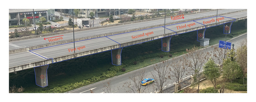
A four-span continuous box-girder concrete bridge is shown in Figure 14. Each span is 25 m, and the deck of bridge is 13 m wide, which are plotted in Figure 15. The main girders are supported by reinforced concrete piers.

The initial FE model of the bridge is established using the ANSYS software according to the design drawings. The main girder of the bridge is modeled using the element SOLID 65. The entire FE model is divided into 65,344 elements, containing 92,928 nodes. Each node has three DOFs, the transverse, longitudinal, and vertical displacements. The DOF number of the entire bridge is 278,784. The elastic modulus and Poisson ratio of the concrete specified in the design drawings are 35 GPa and 0.3, respectively.

5.1. Tests of Bridge Displacements

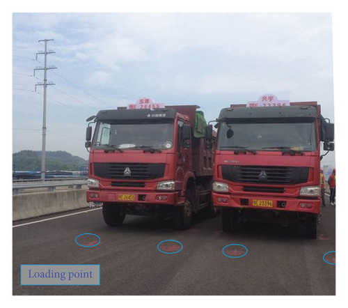
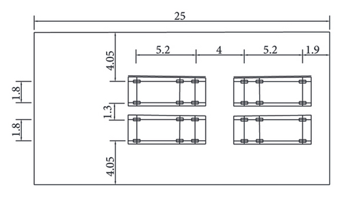
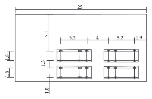
The loading tests conforming to the Chinese testing standard (JTG/T 2015) are performed on the bridge. Four loading vehicles, each weighing 500 kN, are used to distribute loads of 100, 200, and 200 kN at the front, middle, and rear wheel positions, as shown in Figure 16. The loading conditions include Cases 1 to 4. For Cases 1 and 2, the loading is applied to the first span on the left side, where the positions of the loading vehicles are shown in Figure 17. And when the loading is on the second span, the corresponding conditions are Cases 3 and 4.

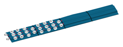
The 24 displacement measurement points including the 6 points at the supporting positions are located at the bottom of the left two spans as depicted in Figure 18. For each loading, the measurement of the displacements is implemented five times. The mean values and COVs of the measured displacements under Cases 1 to 4 are listed in Table 5. It can be observed from Table 5 that due to the influence of the on-site testing environment, the displacement at each measurement point exhibits some degree of uncertainty, where the COVs of the measured displacements range from 0.057 to 0.111. Additionally, it is evident that the maximum relative difference between the measured displacement mean and the initial model displacement reaches 17.27%. Hence, it is necessary to update the FE model of this box-girder bridge.

Table 5. Statistics of the measurement displacements of the continuous box-girder bridge (mm).

	Measured point	A1	B1	C1	A2	B2	C2	A3	B3	C3
Case 1	Initial	2.79	4.70	2.48	2.68	4.55	2.46	2.86	4.76	2.52
	Mean	2.59	4.47	2.35	2.51	4.38	2.35	2.71	4.65	2.42
	Difference	7.72%	5.15%	5.53%	6.77%	3.88%	4.68%	5.54%	2.37%	4.13%
	COV	0.070	0.097	0.067	0.072	0.098	0.079	0.063	0.097	0.073

Case 2	Initial	4.09	6.69	3.71	2.67	4.55	2.45	1.63	3.17	1.52
	Mean	3.98	6.59	3.60	2.51	4.34	2.31	1.44	2.93	1.41
	Difference	−2.76%	−1.52%	−3.06%	−6.37%	−4.84%	−6.06%	−13.19%	−8.19%	−7.80%
	COV	0.076	0.111	0.071	0.087	0.107	0.081	0.071	0.087	0.059

	Measured point	D1	E1	F1	D2	E2	F2	D3	E3	F3

Case 3	Initial	1.79	3.64	2.06	1.76	3.52	2.03	1.81	3.66	2.08
	Mean	1.93	3.71	1.88	1.92	3.63	1.86	1.99	3.75	1.94
	Difference	7.25%	1.89%	−9.57%	8.33%	3.03%	−9.14%	9.05%	2.40%	−7.22%
	COV	0.057	0.074	0.063	0.072	0.087	0.070	0.057	0.084	0.060

Case 4	Initial	2.62	5.57	3.26	1.77	3.52	2.02	1.09	2.33	1.18
	Mean	2.81	5.45	2.78	1.92	3.57	1.85	1.24	2.50	1.19
	Difference	6.76%	−2.20%	−17.27%	7.81%	1.40%	−9.19%	12.10%	6.80%	0.84%
	COV	0.071	0.095	0.072	0.071	0.091	0.075	0.061	0.079	0.072

5.2. Updating of the Bridge

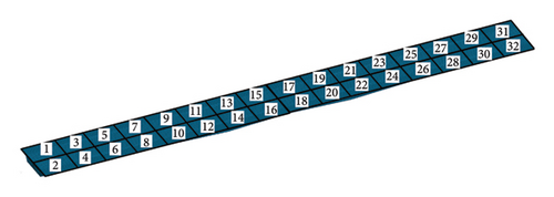
Each span on the left side of the bridge is equally divided into eight regions, leading to 32 regions across the four spans as shown in Figure 19. It is assumed that each region has the same elastic modulus. The updating factors are defined as the rate of change in the elastic modulus of each region relative to its initial design value. Before updating the FE model, the sensitivity values of the displacement responses at the measurement points to the updating factors at the 32 regions are calculated when the loading vehicles are at the first and second spans, respectively, and are plotted in Figures 20(a) and 20(b). Notably, Figure 20(a) shows that the sensitivity values of the displacements at the 8 regions of the first span, as well as the regions 9 and 10 of the second span, are significantly larger than others. Similar phenomenon can be found for the displacements at regions 7 to 18 when the loading is at the second span in Case 2. So, it is proposed to update the FE models of the first and second spans one by one using the measurement displacements.

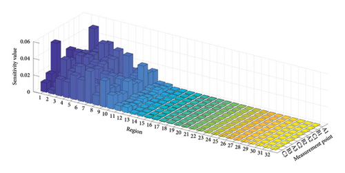
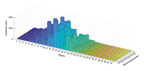
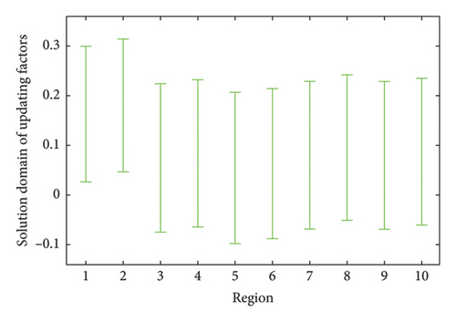
Initially, using the measured displacements in Case 1 and assuming that the updating factors at regions 11 to 32 are zeros according to the sensitivity values in Figure 20(a), the proposed method is used to obtain the updating factors at regions 1 to 10. The solution domains of the updating factors 1 to 10 are computed and drawn in Figure 21. With the aid of these solution domains, equations (36) to (38) are employed to calculate the means and SDs of the updating factors, which are plotted in Figures 22(a) and 22(b), respectively.

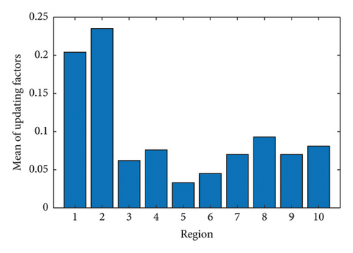
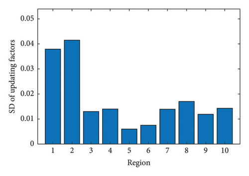
From Figure 22(a), it is observed that the means of the updating factors are all positive, which indicates that there is an underestimation of the elastic modulus values at regions 1 to 10 of the box-girder bridge compared with the design ones. Additionally, from Figure 22(b), it is evident that due to the uncertainty of the measured displacements, the SDs of the 1st to 10th updating factors range from 0.006 to 0.042.

Subsequently, the measured displacements in Case 3 are used to calculate the updating factors 7 to 18. Note that the updating factors 1 to 10 have initially been updated using the measured displacements in Case 1. Considering the union of the initial solutions obtained and the solution domains in Case 3 of the updating factors 7 to 10, the means and SDs of the updating factors 7 to 18 are obtained by the proposed method, as shown in Figure 23.

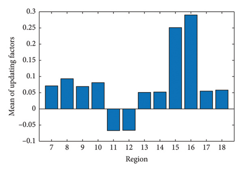
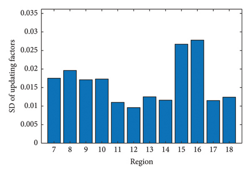
From Figure 23(a), it is seen that most of the mean values of the updating factors are positive. The means of the updating factors 15 and 16 are larger than those of other factors and surpass 0.25. From Figure 23(b), it can be found the SDs of the updating factors change from 0.009 to 0.028. Also, it is watched that the statistics of the updating factors 7 to 10 in Figure 23 are very close to those in Figure 22. Considering the sensitivity values of the displacements in Figure 20, the statistics of the updating factors 7 to 12 in Figure 23 are regarded as the final results.

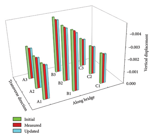
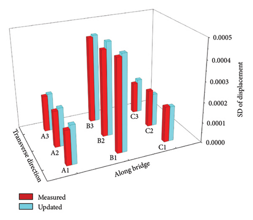
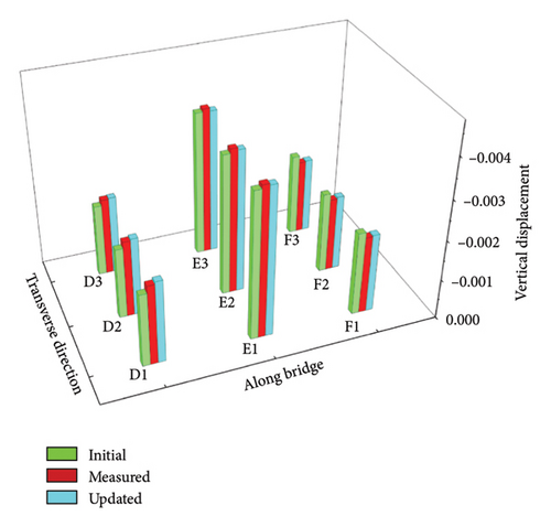
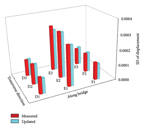
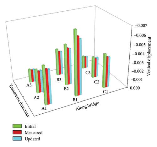
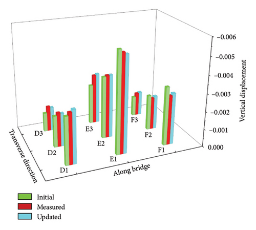
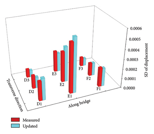
Furthermore, using the updating factors 1 to 18 obtained in Cases 1 and 3, the statistical displacements at the first and second spans of the updated box-girder bridge are calculated and drawn in Figure 24. It is seen from Figure 24(a) that the mean values of the updated displacements at the measurement points of the first span approach those of measured displacements. The maximum relative error between the means of the updated and measured displacements is 0.63%. However, the maximum relative error between the initial displacement values and the means of the measured displacements is 7.72%. Figure 24(b) shows that the SDs of updated displacements agree with those of measured displacements. In Figure 24(c), the maximum relative error between the means of the updated and measured displacements is 1.46%. Figure 24(d) indicates that the maximum relative error between the SDs of the updated and measured displacements is 9.42%.

5.3. Validation of Updating Results

By using the updating factors achieved by the uncertain measurement displacements in Cases 1 and 3, the statistical displacements of the updated bridge are computed under the static loads in Cases 2 and 4 and are graphed in Figures 25 and 26, respectively. It is seen from these two figures that the means and SDs of calculated displacements under static loads agree very well with those of the measured displacements in Cases 2 and 4. It is seen from Figure 25(a) that the mean values of the updated displacements in Case 2 approach those of measured displacements. The maximum relative error between the means of the updated and measured displacements is 4.45%. However, the maximum relative error between the initial displacement values and the means of the measured displacements is 13.19%. From Figure 26(a), it is watched that the maximum relative error between the means of the updated and measured displacements is 4.82%, but the maximum relative error between the means of the initial displacements and measured displacements reaches 17.27%. Figure 26(b) shows that compared with the measured results, the maximum relative error of the SDs of updated displacements is about 20%. These results illustrate that as a whole, the updating factors obtained in Cases 1 and 3 are effective for predicting the displacements in Cases 2 and 4.

About the calculation efficiency of the proposed HSMI method, for each case, the spent time is 12.18 min, and the used computer is the same as that in the second numerical example. Most of the computational time is spent on condensing the 278,784 DOFs of the bridge to 33 DOFs corresponding to the 9 measurement points and 24 loading points. Specially, the calculation of inversion of the matrix K_0bb in equation (39) needs a relatively long time. Fortunately, the sparsity of the stiffness matrix of the bridge greatly accelerates the condensation time.

6. Conclusions

Combining the homotopy method with the pre-estimation technique of solution domains, this paper proposes a new stochastic static model updating method. At first, taking into account the measured static displacements, the solution domains of updating factors in bridge models are derived in terms of the sensitivity of static strain energy. Then the homotopy method is used to transfer the stochastic static model updating equation into a series of deterministic recursive equations about the expansion coefficients of updating factors. Within the estimated solution domains, the expansion coefficients of the updating factors can be solved by the L-curve method and the convex optimization. If the measurement positions do not contain the loading points, a model expansion strategy can be provided.

The frame example demonstrates that, due to the usage of the pre-estimated solution domains, the proposed method can effectively address the ill-posed issue in model updating equations and provide stable updating results, which coincide very well with those assumed real values, in the cases of high-dimension and limited measurement points. In the example of the curved box-girder bridge, it is found that when the displacements at the loading points are not directly measured; compared with the Bayesian method with the FE samples, the proposed method has higher computational efficiency with the equivalent accuracy. When updating a practical continuous box-girder bridge, the proposed method can efficiently update a large FE model, and the statistics of updating results have a good agreement with those of the measured static data.

It is worth noting that currently, the proposed method mainly focuses on the model updating of linearly elastic problems, where the number of measurement points is usually sufficient and measurement errors are well controlled. In the future, the method may be developed to handle nonlinear model updating problems [49].

Disclosure

The authors declare that the final version of this manuscript has been thoroughly reviewed and approved by all coauthors. The authors confirm that the manuscript adheres to the journal′s formatting and publication guidelines.

Furthermore, the authors affirm that this manuscript complies with the ethical standards of academic publishing, including authorship transparency, conflict of interest disclosure, and data integrity.

Conflicts of Interest

The authors declare no conflicts of interest.

Funding

This research was supported by the National Natural Science Foundation of China (51978155) and the China Scholarship Council (202306950129).

Acknowledgments

This research was supported by the National Natural Science Foundation of China (51978155) and the China Scholarship Council (202306950129).

Open Research

Data Availability Statement

The data that support the findings of this study are available on request from the corresponding author. The data are not publicly available due to privacy or ethical restrictions.

References

1 Sanayei M., Bell E. S., Javdekar C. N., Edelmann J. L., and Slavsky E., Damage Localization and Finite-Element Model Updating Using Multiresponse NDT Data, Journal of Bridge Engineering. (2006) 11, no. 6, 688–698, https://doi.org/10.1061/(asce)1084-0702(2006)11:6(688), 2-s2.0-33750121337.
10.1061/(ASCE)1084-0702(2006)11:6(688)
Web of Science® Google Scholar
2 Lu Z. R., Lin X. X., Chen Y. M., and Huang M., Hybrid Sensitivity Matrix for Damage Identification in Axially Functionally Graded Beams, Applied Mathematical Modelling. (2017) 41, 604–617, https://doi.org/10.1016/j.apm.2016.09.008, 2-s2.0-85005950039.
10.1016/j.apm.2016.09.008
Web of Science® Google Scholar
3 Mottershead J. E., Mares C., James S., and Friswell M. I., Stochastic Model Updating: Part 2—application to a Set of Physical Structures, Mechanical Systems and Signal Processing. (2006) 20, no. 8, 2171–2185, https://doi.org/10.1016/j.ymssp.2005.06.007, 2-s2.0-33746997918.
10.1016/j.ymssp.2005.06.007
Web of Science® Google Scholar
4 Chen H., Huang B., Zhang H., Xue K. Y., Sun M., and Wu Z. F., An Efficient Bayesian Method with Intrusive Homotopy Surrogate Model for Stochastic Model Updating, Computer-Aided Civil and Infrastructure Engineering. (2024) 39, no. 16, 2500–2516, https://doi.org/10.1111/mice.13206.
10.1111/mice.13206
Web of Science® Google Scholar
5 Weng S., Xia Y., Zhou X. Q., Xu Y. L., and Zhu H. P., Inverse Substructure Method for Model Updating of Structures, Journal of Sound and Vibration. (2012) 331, no. 25, 5449–5468, https://doi.org/10.1016/j.jsv.2012.07.011, 2-s2.0-84865699575.
10.1016/j.jsv.2012.07.011
Web of Science® Google Scholar
6 Chen H. P. and Tee K. F., Structural Finite Element Model Updating Using Incomplete Ambient Vibration Modal Data, Science China Technological Sciences. (2014) 57, no. 9, 1677–1688, https://doi.org/10.1007/s11431-014-5619-9, 2-s2.0-84920252583.
10.1007/s11431-014-5619-9
Web of Science® Google Scholar
7 Sanayei M., Imbaro G. R., McClain J. A. S., and Brown L. C., Structural Model Updating Using Experimental Static Measurements, Journal of Structural Engineering. (1997) 123, no. 6, 792–798, https://doi.org/10.1061/(asce)0733-9445(1997)123:6(792), 2-s2.0-0031170220.
10.1061/(ASCE)0733-9445(1997)123:6(792)
Web of Science® Google Scholar
8 Sevieri G., Andreini M., De Falco A., and Matthies H. G., Concrete Gravity Dams Model Parameters Updating Using Static Measurements, Engineering Structures. (2019) 196, https://doi.org/10.1016/j.engstruct.2019.05.072, 2-s2.0-85069043465.
10.1016/j.engstruct.2019.05.072
Web of Science® Google Scholar
9 Liu Y., Ma J., Nie J., and Zhang S., Virtual Distortion Method-Based Finite Element Model Updating of Bridges by Using Static Deformation, Journal of Engineering Mechanics. (2017) 143, no. 3, https://doi.org/10.1061/(asce)em.1943-7889.0001006.
10.1061/(ASCE)EM.1943-7889.0001006
Web of Science® Google Scholar
10 Jtg, Load Test Method for Highway Bridge (In Chinese), 2015, China Communication Press, Beijing.
Google Scholar
11 Wu Z. F., Huang B., Fan J., and Chen H., Homotopy Based Stochastic Finite Element Model Updating with Correlated Static Measurement Data, Measurement. (2023) 210, https://doi.org/10.1016/j.measurement.2023.112512.
10.1016/j.measurement.2023.112512
Web of Science® Google Scholar
12 Eberle R. and Oberguggenberger M., A New Method for Estimating the Bending Stiffness Curve of Non-uniform Euler-Bernoulli Beams Using Static Deflection Data, Applied Mathematical Modelling. (2022) 105, 514–533, https://doi.org/10.1016/j.apm.2021.12.042.
10.1016/j.apm.2021.12.042
Web of Science® Google Scholar
13 Martini A., Tronci E. M., Feng M. Q., and Leung R. Y., A Computer Vision-Based Method for Bridge Model Updating Using Displacement Influence Lines, Engineering Structures. (2022) 259, 114129–129, https://doi.org/10.1016/j.engstruct.2022.114129.
10.1016/j.engstruct.2022.114129
Web of Science® Google Scholar
14 Sun R., Wang S., Li M., and Zhu Y., An Algorithm for Large-Span Flexible Bridge Pose Estimation and Multi-Keypoint Vibration Displacement Measurement, Measurement. (2025) 240, https://doi.org/10.1016/j.measurement.2024.115582.
10.1016/j.measurement.2024.115582
Web of Science® Google Scholar
15 Chai S., Wang S., Liu C., Liu X., Liu T., and Yang R., A Visual Measurement Algorithm for Vibration Displacement of Rotating Body Using Semantic Segmentation Network, Expert Systems with Applications. (2024) 237, https://doi.org/10.1016/j.eswa.2023.121306.
10.1016/j.eswa.2023.121306
Web of Science® Google Scholar
16 Zeinali Y. and Story B. A., Impairment Localization and Quantification Using Noisy Static Deformation Influence Lines and Iterative Multi-Parameter Tikhonov Regularization, Mechanical Systems and Signal Processing. (2018) 109, 399–419, https://doi.org/10.1016/j.ymssp.2018.02.036, 2-s2.0-85043992270.
10.1016/j.ymssp.2018.02.036
Web of Science® Google Scholar
17 Bi S. F., Beer M., Cogan S., and Mottershead J., Stochastic Model Updating with Uncertainty Quantification: an Overview and Tutorial, Mechanical Systems and Signal Processing. (2023) 204, https://doi.org/10.1016/j.ymssp.2023.110784.
10.1016/j.ymssp.2023.110784
Web of Science® Google Scholar
18 Sanayei M., Khaloo A., Gul M., and Necati Catbas F., Automated Finite Element Model Updating of a Scale Bridge Model Using Measured Static and Modal Test Data, Engineering Structures. (2015) 102, 66–79, https://doi.org/10.1016/j.engstruct.2015.07.029, 2-s2.0-84939824990.
10.1016/j.engstruct.2015.07.029
Web of Science® Google Scholar
19 Schuëller G. I., Calvi A., Pellissetti M. F., Pradlwarter H. J., Fransen S. H. J. A., and Kreis A., Uncertainty Analysis of a Large-Scale Satellite Finite Element Model, Journal of Spacecraft and Rockets. (2009) 46, no. 1, 191–202, https://doi.org/10.2514/1.32205, 2-s2.0-60349124611.
10.2514/1.32205
Web of Science® Google Scholar
20 Mares C., Mottershead J. E., and Friswell M. I., Stochastic Model Updating: Part 1—theory and Simulated Example, Mechanical Systems and Signal Processing. (2006) 20, no. 7, 1674–1695, https://doi.org/10.1016/j.ymssp.2005.06.006, 2-s2.0-33646533332.
10.1016/j.ymssp.2005.06.006
Web of Science® Google Scholar
21 Zhang H. and Huang B., A New Homotopy-Based Approach for Structural Stochastic Analysis, Probabilistic Engineering Mechanics. (2019) 55, 42–53, https://doi.org/10.1016/j.probengmech.2018.09.001, 2-s2.0-85054733567.
10.1016/j.probengmech.2018.09.001
Web of Science® Google Scholar
22 Beck J. L. and Katafygiotis L. S., Updating Models and Their Uncertainties. I: Bayesian Statistical Framework, Journal of Engineering Mechanics. (1998) 124, no. 4, 455–461, https://doi.org/10.1061/(asce)0733-9399(1998)124:4(455), 2-s2.0-0000235984.
10.1061/(ASCE)0733-9399(1998)124:4(455)
Web of Science® Google Scholar
23 Katafygiotis L. S. and Beck J. L., Updating Models and Their Uncertainties. II: Model Identifiability, Journal of Engineering Mechanics. (1998) 124, no. 4, 463–467, https://doi.org/10.1061/(asce)0733-9399(1998)124:4(463), 2-s2.0-0000235985.
10.1061/(ASCE)0733-9399(1998)124:4(463)
Web of Science® Google Scholar
24 Jia S., Akiyama M., Han B., and Frangopol D. M., Probabilistic Structural Identification and Condition Assessment of Prestressed Concrete Bridges Based on Bayesian Inference Using Deflection Measurements, Structure and Infrastructure Engineering. (2024) 20, no. 1, 131–147, https://doi.org/10.1080/15732479.2023.2192508.
10.1080/15732479.2023.2192508
Web of Science® Google Scholar
25 Jia S., Akiyama M., Han B., Xie H., and Frangopol D. M., Structural Identification via the Inference of the Stochastic Volatility Model Conditioned on the Time-dependent Bridge Deflection, Structural Safety. (2023) 100, https://doi.org/10.1016/j.strusafe.2022.102279.
10.1016/j.strusafe.2022.102279
Web of Science® Google Scholar
26 Liu G. and Jiang W., Model Updating of a Prestressed Concrete Rigid Frame Bridge Using Multiple Markov Chain Monte Carlo Method and Differential Evolution, International Journal of Structural Stability and Dynamics. (2022) 22, no. 03n04, https://doi.org/10.1142/s021945542240020x.
10.1142/S021945542240020X
Web of Science® Google Scholar
27 Zeng J., Kim Y. H., and Qin S., Bayesian Model Updating for Structural Dynamic Applications Combing Differential Evolution Adaptive Metropolis and Kriging Model, Journal of Structural Engineering. (2023) 149, no. 6, https://doi.org/10.1061/jsendh.steng-10837.
10.1061/JSENDH.STENG-10837
Web of Science® Google Scholar
28 Huang B. and Chen H., A New Approach for Stochastic Model Updating Using the Hybrid Perturbation-Garlekin Method, Mechanical Systems and Signal Processing. (2019) 129, 1–19, https://doi.org/10.1016/j.ymssp.2019.04.012, 2-s2.0-85064271933.
10.1016/j.ymssp.2019.04.012
Web of Science® Google Scholar
29 Wu Z. F., Huang B., Chen H., and Zhang H., A New Homotopy Approach for Stochastic Static Model Updating with Large Uncertain Measurement Errors, Applied Mathematical Modelling. (2021) 98, 758–782, https://doi.org/10.1016/j.apm.2021.05.023.
10.1016/j.apm.2021.05.023
Web of Science® Google Scholar
30 Ribeiro D., Calçada R., Delgado R., Brehm M., and Zabel V., Finite Element Model Updating of a Bowstring-Arch Railway Bridge Based on Experimental Modal Parameters, Engineering Structures. (2012) 40, 413–435, https://doi.org/10.1016/j.engstruct.2012.03.013, 2-s2.0-84860500265.
10.1016/j.engstruct.2012.03.013
Web of Science® Google Scholar
31 Na C., Kim S. P., and Kwak H. G., Structural Damage Evaluation Using Genetic Algorithm, Journal of Sound and Vibration. (2011) 330, no. 12, 2772–2783, https://doi.org/10.1016/j.jsv.2011.01.007, 2-s2.0-79953675055.
10.1016/j.jsv.2011.01.007
Web of Science® Google Scholar
32 Astroza R., Nguyen L. T., and Nestorović T., Finite Element Model Updating Using Simulated Annealing Hybridized with Unscented Kalman Filter, Computers & Structures. (2016) 177, 176–191, https://doi.org/10.1016/j.compstruc.2016.09.001, 2-s2.0-84992135197.
10.1016/j.compstruc.2016.09.001
Web of Science® Google Scholar
33 Tran-Ngoc H., Khatir S., De Roeck G., Bui-Tien T., Nguyen-Ngoc L., and Abdel Wahab M., Model Updating for Nam O Bridge Using Particle Swarm Optimization Algorithm and Genetic Algorithm, Sensors. (2018) 18, no. 12, https://doi.org/10.3390/s18124131, 2-s2.0-85057534018.
10.3390/s18124131
Web of Science® Google Scholar
34 Titurus B. and Friswell M. I., Regularization in Model Updating, International Journal for Numerical Methods in Engineering. (2008) 75, no. 4, 440–478, https://doi.org/10.1002/nme.2257, 2-s2.0-48549092658.
10.1002/nme.2257
Web of Science® Google Scholar
35 Calvetti D. and Somersalo E., Inverse Problems: From Regularization to Bayesian Inference, WIREs Computational Statistics. (2018) 10, no. 3, https://doi.org/10.1002/wics.1427, 2-s2.0-85041237639.
10.1002/wics.1427
Google Scholar
36 Zeng C., Thomas D. C., and Lewinger J. P., Incorporating Prior Knowledge into Regularized Regression, Bioinformatics. (2021) 37, no. 4, 514–521, https://doi.org/10.1093/bioinformatics/btaa776.
10.1093/bioinformatics/btaa776
CAS PubMed Web of Science® Google Scholar
37 Ortega-Culaciati F., Simons M., Ruiz J., Rivera L., and Díaz-Salazar N., An Epic Tikhonov Regularization: Application to Quasi-static Fault Slip Inversion, Journal of Geophysical Research: Solid Earth. (2021) 126, no. 7, https://doi.org/10.1029/2020jb021141.
10.1029/2020JB021141
Web of Science® Google Scholar
38 Renaut R. A., Hnětynková I., and Mead J., Regularization Parameter Estimation for Large-Scale Tikhonov Regularization Using A Priori Information, Computational Statistics & Data Analysis. (2010) 54, no. 12, 3430–3445, https://doi.org/10.1016/j.csda.2009.05.026, 2-s2.0-78049324264.
10.1016/j.csda.2009.05.026
Web of Science® Google Scholar
39 Xie D., Lu Z. R., Li G., Liu J., and Wang L., Efficient Laplace Prior-Based Sparse Bayesian Learning for Structural Damage Identification and Uncertainty Quantification, Mechanical Systems and Signal Processing. (2023) 188, https://doi.org/10.1016/j.ymssp.2022.110000.
10.1016/j.ymssp.2022.110000
Web of Science® Google Scholar
40 Zhang C. D. and Xu Y. L., Comparative Studies on Damage Identification with Tikhonov Regularization and Sparse Regularization, Structural Control and Health Monitoring. (2016) 23, no. 3, 560–579, https://doi.org/10.1002/stc.1785, 2-s2.0-84956726877.
10.1002/stc.1785
Web of Science® Google Scholar
41 Gholami A. and Siahkoohi H. R., Simultaneous Constraining of Model and Data Smoothness for Regularization of Geophysical Inverse Problems, Geophysical Journal International. (2009) 176, no. 1, 151–163, https://doi.org/10.1111/j.1365-246x.2008.03949.x, 2-s2.0-58149185270.
10.1111/j.1365-246X.2008.03949.x
Web of Science® Google Scholar
42 Gülçehre Ç. and Bengio Y., Knowledge Matters: Importance of Prior Information for Optimization, The Journal of Machine Learning Research. (2016) 17, no. 1, 226–257.
Web of Science® Google Scholar
43 Seyedpoor S. M. and Yazdanpanah O., An Efficient Indicator for Structural Damage Localization Using the Change of Strain Energy Based on Static Noisy Data, Applied Mathematical Modelling. (2014) 38, no. 9-10, 2661–2672, https://doi.org/10.1016/j.apm.2013.10.072, 2-s2.0-84898540365.
10.1016/j.apm.2013.10.072
Web of Science® Google Scholar
44 Hua X. G., Ni Y. Q., Chen Z. Q., and Ko J. M., An Improved Perturbation Method for Stochastic Finite Element Model Updating, International Journal for Numerical Methods in Engineering. (2008) 73, no. 13, 1845–1864, https://doi.org/10.1002/nme.2151, 2-s2.0-41449111984.
10.1002/nme.2151
Web of Science® Google Scholar
45 Reumers P., Van hoorickx C., Schevenels M., and Lombaert G., Density Filtering Regularization of Finite Element Model Updating Problems, Mechanical Systems and Signal Processing. (2019) 128, 282–294, https://doi.org/10.1016/j.ymssp.2019.03.038, 2-s2.0-85063889666.
10.1016/j.ymssp.2019.03.038
Web of Science® Google Scholar
46 Burger M., Resmerita E., and He L., Error Estimation for Bregman Iterations and Inverse Scale Space Methods in Image Restoration, Computing. (2007) 81, no. 2-3, 109–135, https://doi.org/10.1007/s00607-007-0245-z, 2-s2.0-36549078210.
10.1007/s00607-007-0245-z
Web of Science® Google Scholar
47 Kaltenbacher B., Neubauer A., and Scherzer O., Iterative Regularization Methods for Nonlinear Ill-Posed Problems, 2008, De Gruyter, Berlin, New York.
10.1515/9783110208276
Web of Science® Google Scholar
48 Grant M., Boyd S., and Ye Y., CVX Users’ Guide, 2009, http://www.stanford.edu/boyd/software.html.
Google Scholar
49 Zhang H., Xiang X., Huang B., Wu Z. F., and Chen H., Static Homotopy Response Analysis of Structure with Random Variables of Arbitrary Distributions by Minimizing Stochastic Residual Error, Computers & Structures. (2023) 288, https://doi.org/10.1016/j.compstruc.2023.107153.
10.1016/j.compstruc.2023.107153
Web of Science® Google Scholar

All articles

Stochastic Static Model Updating of Bridge Using Homotopy Method and Pre-Estimated Solution Domain

Abstract

1. Introduction

2. Theoretical Frameworks

2.1. Pre-Estimation of Solution Domains of Updating Factors

2.2. Homotopy Approach for the Updating Factors

2.3. Solutions of Recursive Equations Using the L-Curve Method and Convex Optimization

2.4. Expansion of Measurement Displacement Vector

3. Numerical Example I: One Single Story Frame

4. Numerical Example II: A Curved Bridge With Single Box and Single Cell