Evaluating Measurement System Capability in Condition Monitoring: Framework and Illustration Using Gage Repeatability and Reproducibility
Abstract
In condition monitoring, the reliability of a predictive maintenance program is critically dependent on the precision of data obtained from measurement systems. With increased availability, a significant challenge is evaluating the capability of these measurement systems to ensure data precision, which is fundamental for informed system selection. To address this challenge, this study proposes a systematic framework for evaluating the capability of these measurement systems using Gage repeatability and reproducibility (Gage R&R) technique, subsequently judging the acceptability level and guiding their selection to guarantee the data precision. Our study investigates the capability of these systems in terms of repeatability and reproducibility, quantifying the contributions of different sources to the systems’ capability and providing directions for measurement system correction and enhancement. Another distinctive innovation of our approach is the use of three-region graphs, incorporating metrics including percentage of Gage R&R to total variation, precision-to-tolerance ratio, and signal-to-noise ratio, which presents a comprehensive overview of the systems’ capability within one single figure. Two comparative experiments in distinct application scenarios were conducted to validate the effectiveness of the proposed framework. The insights presented serve as a valuable reference to replace the commonly used experience-based system selection in condition monitoring. Through this framework, we present a promising data-based approach aimed at enhancing the widely employed time-based calibration strategies, ultimately contributing to the improvement of data quality and the overall success of condition monitoring initiatives.
1. Introduction
With the rapid development of the Internet of Things (IoT), condition monitoring (CM) has gained paramount significance across various fields as a process of monitoring the equipment or structural condition to detect changes that may indicate a potential failure [1, 2]. CM system plays a crucial role in implementing a reliable predictive maintenance program, providing real-time insight into equipment or structural health and enabling timely maintenance scheduling. Central to CM’s reliability is the overarching importance of data quality. Heightened data precision invariably leads to enhanced data quality, and this direct correlation necessitates a robust assurance mechanism, especially in the context of predictive maintenance.
Among various measurement systems used in CM, vibration measurement system (VMS) and acoustic emission measurement system (AEMS) have attracted increasing interest due to their capability not only for early fault detection but also for providing higher accuracy in identifying faults [3, 4]. When building a new measurement system and utilizing the measured data to develop maintenance strategies in CM, the accuracy of data becomes paramount and depends largely on the capability of the measurement system. However, most studies assume the measurement systems are capable and acceptable without proper justification in CM, which may ultimately lead to questionable maintenance decisions [5, 6]. Recent studies have greatly advanced our understanding of the significance of measurement system’s performance. Mobaraki et al. [7] investigated the impacts of test conditions and nonoptimal positioning of the sensors on the accuracy of the measurements. Rackes et al. [8] conducted a comparative analysis of three sensors in different office environments using Monte Carlo analysis. Liang et al. [9] explored the performances of LoRa in buildings, focusing on network transmission delay and packet loss rate. Meserkhani et al. [10] offered experimental comparisons in rolling bearing fault diagnosis using different AE sensors. Liu et al. [11] examined sensor performance in source localization on plate structures using piezoelectric fiber composites.
Despite these advancements, most studies primarily focus on evaluating measurement system accuracy, often overlooking the influence of variables such as measured objects and operators, which are crucial for thorough and reliable capability assessments. The Gage repeatability and reproducibility (Gage R&R [GRR]) technique, acknowledging the effects of the measurement system, objects, and operators, is a well-established method for determining acceptable system variability [12]. For instance, Chen et al. [13] proposed an integrated scheme to evaluate the capability of different sensors using GRR. Asplund et al. [14] utilized GRR to evaluate a wheel profile measurement system in a railway network, while Shirodkar et al. [15] examined the reliability of measurements influenced by changes in location, probe radius, and touch speed using GRR.
While GRR has been widely applied to assess the capability of the measurement system and identify the root causes of measurement errors in various fields [16–19], a definitive solution for appraising the capability of the measurement systems has yet to emerge in CM, which often results in data inaccuracies and increased operational costs in practical applications. Thus, there comes a crucial research question: How can we effectively evaluate measurement systems’ capability to provide a reference for an informed system selection to guarantee data precision in CM?
This study develops an advanced framework that innovatively applies the GRR technique to assess measurement system capability in CM. We propose a structured validation framework to address the lack of systematic evaluation methodologies in the current study, enhancing decision-making in system selection and optimization. Our research also investigates key factors influencing measurement precision, providing insights to mitigate variability and improve accuracy. To facilitate assessment, we introduce a novel three-region graphical representation, enabling clear comparisons of different measurement systems. Additionally, we integrate a data-driven approach to supplement traditional calibration strategies, allowing dynamic schedule adjustments based on real-time performance data, ensuring continuous accuracy and reducing system degradation risks. Furthermore, this study lays the foundation for real-time capability evaluation, contributing to intelligent, adaptive monitoring solutions that enhance long-term reliability. By addressing a critical gap in measurement system evaluation, our research advances precision in measurement science while offering a transformative perspective on system selection, calibration, and reliability assurance in CM.
This reminder of the paper is organized as follows. Section 2 provides an overview of the study’s framework. Sections 3 and 4 collectively illustrate and validate this framework, with Section 3 detailing the experimental study’s background and Section 4 presenting and analyzing the experimental results. In Section 5, discussions of the study’s findings along with critical comments and recommendations are provided. The paper concludes with Section 6, where we summarize the key conclusions drawn from our research.
2. Framework for Measurement System Capability Evaluation
In this section, we propose a comprehensive evaluation framework specifically designed for assessing the capability of measurement systems used in CM. This framework is the cornerstone of our methodology, focusing on the capability evaluation of VMS and AEMS, which are essential in the field of machinery and structural health monitoring.
This framework also serves as a practical guideline for evaluating the capability of measurement systems in diverse scenarios. By systematically breaking down each component of the evaluation process, we aim to offer a replicable and robust model that enhances the generalizability of the framework.
2.1. Measurement System Capability Evaluation Procedure
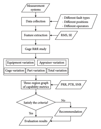
The procedure of the measurement system capability evaluation is shown in Figure 1. The procedure starts with collecting data of various fault types from different measurement positions by different operators using the measurement system. In this study, we illustrate the proposed framework by using a machinery faulty system as a case study. In doing so, we utilize specific combinations of fault types and measurement positions as our designated measurement “parts” which are important and typical for the measured experimental setups. Then, two features root mean square (RMS) and spectral energy (SE) are extracted to characterize the machinery conditions. We then conduct a GRR study to compute the variations of different sources, including equipment variation (EV), appraiser variation (AV), GRR, part variation (PV), and total variation (TV). Subsequently, the three-region graphs are designed to give a good overview with three metrics, including percentage of GRR to total variation (PRR), precision-to-tolerance ratio (PTR), and signal-to-noise ratio (SNR), in the same figure and provide a clear way of seeing the capability of the measurement system. The section concludes with guidelines for selecting and improving measurement systems.
2.2. Feature Extraction
In this study, we employ statistical features such as RMS and SE to characterize the measurement data from both VMS and AEMS. These particular features have been demonstrated in effectively describing the characteristics of vibration and AE signals, as referenced in studies [20–23].
2.2.1. RMS
2.2.2. SE
2.3. GRR Study
The GRR study is carried out to evaluate the extent of variability of the measurement system considering both repeatability and reproducibility. A minimal variation of measurement data serves as a good indicator of the measurement system’s precision. The GRR study is performed using analysis of variance (ANOVA), as it offers a more precise depiction of the variations inherent in the measurement system [24].
2.3.1. AV
2.3.2. PV
2.3.3. EV
2.3.4. GRR
2.3.5. TV
2.4. Capability Metrics
This section introduces key metrics used to evaluate the measurement system’s capability.
2.4.1. PRR
| Evaluation | Values | Comments |
|---|---|---|
| Good | < 10% | The measurement system is capable. |
| Conditionally acceptable | 10%–30% | The measurement system may be capable depending on the requirement. |
| Unacceptable | > 30% | The measurement system is not capable and needs improvement. |
2.4.2. PTR
| Evaluation | Values | Comments |
|---|---|---|
| Good | < 0.1 | The measurement system is capable. |
| Conditionally acceptable | 0.1–0.3 | The measurement system may be capable depending on the requirement. |
| Unacceptable | > 0.3 | The measurement system is not capable and needs improvement. |
2.4.3. SNR
| Evaluation | Values | Comments |
|---|---|---|
| Good | ≥ 10 | The measurement system is capable. |
| Conditionally acceptable | 5–10 | The measurement system may be capable depending on the requirement. |
| Unacceptable | < 5 | The measurement system is not capable and needs improvement. |
3. Experimental Setup: Framework Implementation
In this section, we provide a comprehensive overview of the measurement systems’ components and configurations, ensuring a thorough understanding of the research objects in our experiments. Following this, we describe the test bench setup utilized to simulate various fault types in CM applications. This setup is pivotal in testing the capability of the measurement systems under different scenarios, thereby offering a robust platform for validating our framework. It is through this experimental implementation that we bring the theoretical aspects of the framework to practice, demonstrating its potential in industrial applications.
3.1. Introduction to the Measurement Systems
As a pivotal part of this study, we constructed two widely used measurement systems in CM applications to validate our proposed framework, which are the VMS and the AEMS. Each system is comprised of four fundamental components: sensors, data transmission, data acquisition, and data display, as detailed in Figures 2 and 3. The comprehensive details regarding each component in the VMS and AEMS can be found in Tables 4 and 5.


| Components | Manufacturer | Model no. | Specification |
|---|---|---|---|
| Sensor: accelerometer | PCB | 333B30 | Sensitivity: 10.2 mV/(m/s2); measurement range: ±50 g; frequency range: 0.5–3000 Hz |
| Data transmission: cables |
|
|
|
| Data acquisition: A/D card | B&K | LAN-XI 3053 |
|
| Data display: storage and processing | ThinkPad | X1 Carbon | CPU Core i7 6600U, 16 GB RAM |
| Components | Manufacturer | Model no. | Specification |
|---|---|---|---|
| Sensor: AE sensor | PAC | PK15I |
|
| Data transmission: cables | Eastsheep | SMA/BNC-JJ | SMA to BNC cable |
| Data acquisition: A/D card | NI | USB-6356 |
|
| Data display: storage and processing | ThinkPad | X1 Carbon | CPU Core i7 6600U, 16 GB RAM |
3.2. Introduction to the Test Bench
To comprehensively validate the effectiveness and robustness of the proposed framework, we conducted two comparative experiments in distinct industrial application scenarios. The first experiment, a rotor fault diagnosis test, was carried out in a laboratory environment. The second experiment, focusing on wheelset fault detection, was conducted in an actual enterprise setting.
3.2.1. Rotor Fault Test Bench
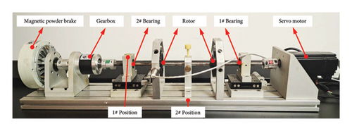
Figure 4 displays the rotor fault test bench, consisting of servo motor, bearings, rotor, gearbox, coupling, and magnetic powder brake. Two rolling bearings were used in the experiment: 1# bearing, in a normal condition, and 2# bearing, exhibiting three distinct fault types—compound faults (inner and outer race defects), ball faults, and cage faults. Detailed information about the rolling bearings is outlined in Table 6. The sensors are strategically placed adjacent to each other on the base at two distinct locations: 1# and 2# positions as depicted in Figure 4. It is worth noting that the sampling frequency (SF) is configured at 32,768 and 500,000 Hz for the VMS and the AEMS, respectively, ensuring comprehensive signal acquisition in our experiments.
| Parameters | Ball diameter (mm) | Inner diameter (mm) | Outer diameter (mm) | Width (mm) | Ball number |
|---|---|---|---|---|---|
| Value | 5.6 | 10 | 30 | 9 | 8 |
The data acquired from three fault types and two measurement positions are considered as six different “parts.” Conducting these experiments, three operators each performed 20 trials for every part using both VMS and AEMS. The rotor speed was set to 500 rpm, and each measurement captured 5 revolutions of state information, integrating various fault types, measurement locations, and operators. This yields a total of 360 measurements, with each measurement containing 19,660 and 300,000 data points for the VMS and AEMS, respectively.
3.2.2. Wheelset Fault Test Bench
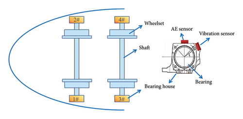
Figure 5 presents the schematic diagram of the wheelset fault test bench, which comprises wheelsets, bearings, a shaft, and bearing housings. The experiment utilized four tapered roller bearings with varying health conditions: Bearing #1 in normal condition, Bearing #2 with a mild outer race fault, Bearing #3 with a moderate outer race fault, and Bearing #4 with a severe outer race fault. Detailed specifications of the rolling bearings are provided in Table 7. To ensure precise signal acquisition, sensors were strategically positioned in close proximity on the bearing housings, as illustrated in Figure 5. The SFs were set at 2.56 kHz for the VMS and 2 MHz for the AEMS, enabling comprehensive data collection.
| Parameters | Roller diameter (mm) | Inner diameter (mm) | Outer diameter (mm) | Pitch diameter (mm) | Ball number |
|---|---|---|---|---|---|
| Value | 26 | 130 | 230 | 183.929 | 19 |
For each fault type, the acquired data were categorized into four distinct “parts.” In the experimental procedure, three operators conducted six trials per part using both VMS and AEMS. The shaft speed was maintained at 2160 rpm, with each measurement capturing two complete revolutions of state information. This setup effectively integrates multiple fault conditions and operator variations, ensuring the robustness and reliability of the experimental dataset.
4. Results Analysis: Framework Validation
In this section, we delve into a detailed analysis of the experimental results, focusing on validating the effectiveness and robustness of our framework. We examine variations in key features, analyze the GRR results, and evaluate crucial metrics to ascertain the capability of both VMS and AEMS. This analysis not only demonstrates the practical applicability of our framework but also provides insightful conclusions on the measurement systems’ capability.
4.1. Variation of Features
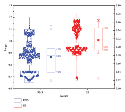
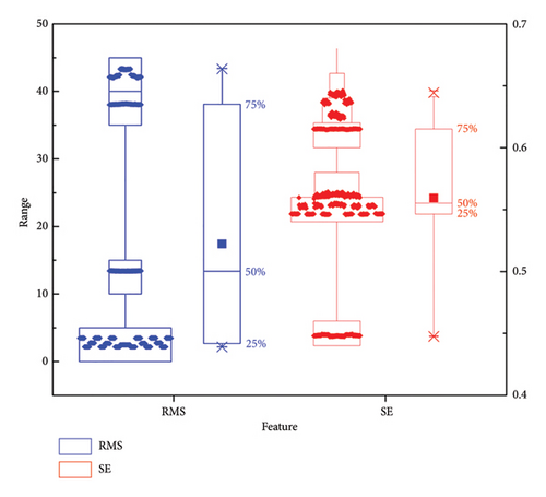
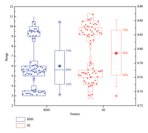
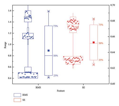
The boxplots of features RMS and SE for both VMS and AEMS in two different experiments are displayed in Figures 6, 7, 8, and 9, respectively. The features of these measurements allow us to analyze variations arising from the measurement systems, operators, and parts. Notably, the dispersion of two features varies significantly for the two measurement systems, with the VMS exhibiting higher dispersion compared to the AEMS under both tests, indicating that the variation of the data measured with VMS is greater than that of AEMS. Furthermore, the amplitude variations of RMS are notably larger than those of SE, indicating distinct disparities in feature behaviors between the two systems. It also should be noteworthy that the feature SE demonstrates greater robustness to variations in operating conditions compared to the feature RMS, which exhibits higher susceptibility to such changes. It is observed that the clustering of features is more concentrated in Experiment II. This can be attributed to the fact that fault characteristics become more pronounced at higher speeds, leading to improved clustering. This finding also indicates that both features are capable of accurately distinguishing between different operating conditions, effectively characterizing the system’s varying states. As a result, SE is a more reliable indicator for characterizing the capability of the measurement system, making it preferable over RMS in this context.
4.2. GRR Results
The GRR analysis results for both VMS and AEMS in two comparative experiments are shown in Tables 8 and 9, respectively. The SD, percentage of variance (PVA), and percentage of study variation (PSV) for features RMS and SE are calculated in terms of five sources: EV, AV, GRR, PV, and TV. GRR represents the variations arising from both operators and measurement system during the measurement process, which is a pivotal parameter in characterizing the measurement system’s precision. The SD, PVA, and PSV values exhibit variabilities depending on the different measurement systems, features, speeds, and sources involved. It is noteworthy, for feature RMS, the VMS consistently produces lower SD values compared to the AEMS under two different experiments. However, when examining the feature SE, the SD values of both measurement systems are relatively close. Moreover, the PVA, PSV, and their respective average values for source GRR are considerably lower for the AEMS compared to the VMS when considering both features. The average SD, PVA, and PSV values for AV are higher than those for EV in Experiment I, suggesting that operator is an indispensable influence factor on the capability of measurement system. The SD values in Experiment I are lower than those observed in Experiment II, which can be attributed to the greater vibration interference present at the higher speed. This increased interference in Experiment II leads to more significant fluctuations in SD values, reflecting the system’s heightened variability under such conditions. The PVA, PSV, and their average values of both features for source PV are close to 100%, highlighting PV serves as the primary factor in the TV. Another noteworthy observation is that the combination of GRR and PV, resulting in TV, sums up to 100%, indicating the comprehensiveness of our analysis in considering all sources of variation.
| Features | Sources | Experiment I | Experiment II | ||||
|---|---|---|---|---|---|---|---|
| SD | PVA (%) | PSV (%) | SD | PVA (%) | PSV (%) | ||
| RMS | EV | 0.019 | 1.9 | 13.9 | 0.262 | 1 | 10.2 |
| AV | 0.023 | 2.8 | 16.8 | 0.287 | 1.3 | 11.2 | |
| GRR | 0.029 | 4.7 | 21.8 | 0.388 | 2.3 | 15.1 | |
| PV | 0.131 | 95.3 | 97.6 | 2.54 | 97.7 | 98.85 | |
| TV | 0.135 | 100 | 100 | 2.57 | 100 | 100 | |
| SE | EV | 0.0027 | 0.7 | 8.4 | 0.0087 | 4.5 | 21.3 |
| AV | 0.0036 | 1.3 | 11.4 | 0.0062 | 2.3 | 15.2 | |
| GRR | 0.0045 | 2 | 14.1 | 0.0106 | 6.8 | 26.2 | |
| PV | 0.0312 | 98 | 99 | 0.0393 | 93.2 | 96.5 | |
| TV | 0.0315 | 100 | 100 | 0.0407 | 100 | 100 | |
| Average | EV | 0.011 | 1.3 | 11.2 | 0.135 | 2.75 | 15.7 |
| AV | 0.013 | 2.1 | 14.1 | 0.147 | 1.8 | 13.2 | |
| GRR | 0.017 | 3.4 | 18 | 0.199 | 4.6 | 20.6 | |
| PV | 0.081 | 96.7 | 98.3 | 1.29 | 95.4 | 97.7 | |
| TV | 0.083 | 100 | 100 | 1.31 | 100 | 100 | |
| Features | Sources | Experiment I | Experiment II | ||||
|---|---|---|---|---|---|---|---|
| SD | PVA (%) | PSV (%) | SD | PVA (%) | PSV (%) | ||
| RMS | EV | 0.02 | 0.0001 | 0.11 | 0.029 | 0.32 | 5.67 |
| AV | 0.2737 | 0.0218 | 1.47 | 0.001 | 0.002 | 0.21 | |
| GRR | 0.2744 | 0.0219 | 1.48 | 0.0297 | 0.322 | 5.674 | |
| PV | 18.56 | 99.98 | 99.99 | 0.522 | 99.68 | 99.84 | |
| TV | 18.56 | 100 | 100 | 0.523 | 100 | 100 | |
| SE | EV | 0.0006 | 0.01 | 0.1 | 0.0022 | 0.718 | 8.47 |
| AV | 0.0037 | 0.321 | 5.67 | 0.0002 | 0.002 | 0.58 | |
| GRR | 0.0038 | 0.331 | 5.75 | 0.0023 | 0.72 | 8.49 | |
| PV | 0.0653 | 99.67 | 99.83 | 0.0261 | 99.28 | 99.64 | |
| TV | 0.0654 | 100 | 100 | 0.0262 | 100 | 100 | |
| Average | EV | 0.01 | 0.01 | 0.1 | 0.0156 | 0.519 | 7.07 |
| AV | 0.139 | 0.17 | 3.57 | 0.0006 | 0.002 | 0.4 | |
| GRR | 0.14 | 0.18 | 3.6 | 0.016 | 0.521 | 7.1 | |
| PV | 9.31 | 99.83 | 99.91 | 0.274 | 99.48 | 99.74 | |
| TV | 9.31 | 100 | 100 | 0.275 | 100 | 100 | |
4.3. Metrics Evaluation
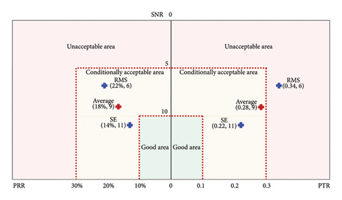
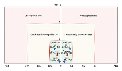
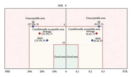
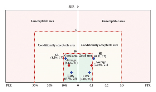
The metrics are influenced by the USL and LSL of the features. In this study, we calculate the limits of these features using the observed history data, employing a critical value of 1.96 for a 95% confidence interval. The LSL, USL, and tolerance of features RMS and SE for both measurement systems in two experiments are outlined in Tables 10 and 11, respectively. The three-region graph is utilized to show the acceptable levels of the metrics, enhancing the visualization of the measuring system capability by categorizing it into three zones: “unacceptable area,” “conditionally acceptable area,” or “good area.” This type of graph not only provides a clear display of the acceptability of the measurement system but also shows the multiple metrics in the same graph without being difficult to interpret. Figures 10 and 11 show this type of three-region graphs of metrics for the VMS and AEMS in Experiment I, respectively. The horizontal axis represents the values of PRR and PTR, while the vertical axis corresponds to SNR values. The limits of the graphs are determined by the values provided in Tables 1, 2, and 3. As displayed in Figure 10, the average capability metrics of the VMS are deemed conditionally acceptable, with all the metrics for feature SE falling within the conditionally acceptable category while the metric PTR for feature RMS lying in the unacceptable region. As shown in Figure 11, the average capability metrics of the AEMS fall within the good area, and all the metrics for both features are situated in the acceptable region. Interestingly, the metrics values of feature SE are lower than those of features RMS for VMS, while it is the opposite for the AEMS–SE metrics values which are higher than those of RMS. Figures 12 and 13 present the three-region graphs of metrics for the VMS and AEMS in Experiment II, respectively. As illustrated in Figure 12, the capability metrics of the VMS are deemed conditionally acceptable, with all evaluated metrics for both the features SE and RMS falling within the conditionally acceptable range. This indicates that, while the system performs adequately under the given conditions, there is potential for further optimization to achieve fully acceptable performance. As demonstrated in Figure 13, the average capability metrics of the AEMS fall within the “good” performance area, with all metrics for both features positioned within the acceptable region. This suggests that the AEMS exhibits strong measurement capability under the evaluated conditions. This observation indicates that the measurement capability of the AEMS generally surpasses that of the VMS when evaluated under the same feature criteria and speed conditions.
| Systems | Features | LSL | USL | Tolerance |
|---|---|---|---|---|
| VMS | RMS | 0.6 | 1.1 | 0.5 |
| SE | 0.7 | 0.8 | 0.1 | |
| AEMS | RMS | 0 | 51 | 51 |
| SE | 0.4 | 0.7 | 0.3 | |
| Systems | Features | LSL | USL | Tolerance |
|---|---|---|---|---|
| VMS | RMS | 1.6 | 10.4 | 8.8 |
| SE | 0.7 | 0.9 | 0.2 | |
| AEMS | RMS | 0 | 1.8 | 1.8 |
| SE | 0.6 | 0.7 | 0.1 | |
5. Discussion and Recommendations
In this section, we will discuss the insights and implications derived from our comprehensive evaluation results of the VMS and AEMS.
5.1. Discussion on Measurement System Capability
According to the experimental findings, both VMS and AEMS exhibit distinct measurement capabilities, noticeable in the variations concerning features RMS and SE, as depicted in Tables 8 and 9. An interesting observation is that the capability evaluation results for different features are different, even if they come from the same measurement system. The reason lies in the specific characteristics required by different measurement systems for accurate characterization. Moreover, the variations of results are associated with the dispersion of the features which is due to the different properties of the measurement systems. Notably, compared to the feature SE, the feature RMS is more susceptible to fluctuations in different operating conditions. Therefore, the feature selection plays a pivotal role in the capability evaluation of the measurement system, imposing a substantial influence on the evaluation results.
The three-region graphs provide a clear visualization of the capability and acceptability for both VMS and AEMS in two experiments as displayed in Figures 10, 11, 12, 13. These graphs make the evaluation easy to interpret and provide an indication of the capability levels of different measurement systems. The metric PRR measures the variance of the measurement system, PTR is rooted in the variance ratio between the measurement system and the part, while the SNR is dependent on the part variance. The results reveal that the metrics PRR, PTR, and SNR of feature SE are within the conditionally acceptable area for the VMS. For feature RMS, the metrics PRR and SNR for the VMS fall in the conditionally acceptable region in two experiments, while the PTR metric is considered unacceptable in Experiment I and conditionally acceptable in Experiment II. However, all the capability metrics of the AEMS for both features in the two experiments are situated in the acceptable region, suggesting that the capability of the AEMS is not only acceptable but also well suited for the intended application in this study, while the VMS can be employed for the applications conditionally depending on the factors such as importance, risk, cost, and operation conditions. Obviously, there is a contradiction between different features and metrics, and the evaluation results based on these metrics will be contradictory depending on the established criteria. To avoid the issue, it is advisable to select the suitable features and the metrics with the highest credibility depending on the desired performance and the specific application of the measurement. Adjusting the limits of USL and LSL may be a feasible strategy to resolve these contradictions.
5.2. Recommendations and Comments
The experimental results confirm the superior capability of the AEMS, which consistently outperforms the VMS across all metrics, consistently falling within the “good areas” for precise measurement applications. The GRR results presented in Tables 8 and 9 highlight a significant portion of measurement variation when employing the VMS, particularly stemming from the sources EV and AV. To ensure accurate measurements, it is crucial to take corrective actions that address both the measurement system (e.g., replace sensor or acquisition card) and operator-related factors (e.g., check operation specifications, installation positions, or environmental interference). Our study provides an invaluable reference for an informed system selection in CM scenarios demanding high precision. Considering our findings, we recommend ongoing capability evaluation of measurement systems, especially in dynamic industrial environments, enhancing the commonly used time-based system calibration strategy.
The variability of the measurement system includes both repeatability and reproducibility which need comprehensive investigation to ensure the high precision of the measurement system. Nevertheless, the evaluation results should not be solely dependent on a single metric or measurement variations. Each application should be analyzed individually, considering specific requirements and the contexts of measurement use. Furthermore, when assessing capability in practical applications, the long-term performance of measurement system should be a key consideration to ensure consistent and reliable results over time.
The proposed framework has the potential for additional extension into the online capability evaluation of measurement systems, offering a substitute from traditional periodic evaluations. This extension has significant implications in the field of machinery and structural health monitoring, not only helping to minimize downtime but also improving data quality and reliability. When applied in faultless scenarios, we recommend considering various combinations of measurement time, positions, and operating conditions as different “parts” in the data collection stage.
6. Conclusion
This study has successfully developed a systematic framework to address the critical research concern of evaluating the capability of measurement systems for precise and reliable data acquisition in CM applications. The innovative framework, tailored for CM applications, marks a paradigm shift from traditional experience-based system selection and time-based calibration strategies to a data-driven approach, offering invaluable guidance for CM practitioners. A significant highlight of our evaluation is the utilization of three-region graphs, offering a comprehensive overview of various metrics within a single figure. Notably, the VMS exhibits conditionally acceptable capability in features RMS and SE, while the AEMS consistently surpasses predefined criteria, making it a more favorable choice in this context. To enhance VMS capability, we recommend a thorough reengineering of the measurement system.
However, our findings reveal contradictions in evaluation results when different features and metrics are employed. In some instances, one metric may indicate conditionally acceptable capability while another suggests unacceptable levels. This emphasizes the critical importance of features and metrics selection in evaluating measurement system capability. This study is centered on evaluating the capability of the measurement system from the perspective of data precision. It serves as a valuable reference for guiding the appropriate selection of measurement systems, but it should not be considered the sole criterion for such selection.
Looking forward, future research efforts should focus on identifying the most suitable features and metrics to precisely characterize the capabilities of measurement systems. Additionally, investigations in the field of online capability evaluation for measurement systems are warranted. Such research can contribute to the development of timely calibration strategies, ensuring sustained data quality and reliability in measurement systems. Regular and ongoing evaluation studies are recommended to maintain data quality, as well as the precision of the measurement system in long-term CM applications.
In summary, this study not only addresses a critical research question in CM but also offers practical solutions and forward-looking perspectives for the selection and calibration of measurement systems. By continuously monitoring and evaluating these systems, industries can ensure the deployment of efficient tools for reliable predictive maintenance, ultimately enhancing the overall success of CM initiatives.
Conflicts of Interest
The authors declare no conflicts of interest.
Funding
The research was funded by Qingdao Postdoctoral Program (QDBSH20240202010), Shandong Postdoctoral Innovation Program and Shandong Provincial Natural Science Foundation (grant no. ZR2020ME124). The authors sincerely thank Luleå University of Technology and Qingdao Huihezhongcheng Intelligent Science and Technology Co. Ltd. for their support in terms of funding and experimental equipment.
Acknowledgments
The authors sincerely thank Luleå University of Technology and Qingdao Huihezhongcheng Intelligent Science and Technology Co. Ltd. for their support in terms of funding and experimental equipment. Furthermore, the authors express gratitude to the anonymous reviewers for their valuable comments, which greatly improved the quality of the article.
Open Research
Data Availability Statement
The data used to support the findings of this study were supplied by Qingdao Huihe Zhongcheng Intelligent Technology Ltd under license and so cannot be made freely available. Requests for access to these data should be made to Haizhou Chen, [email protected].


