Prediction of Surrounding Rock Deformation in a Highway Tunnel Using an LSTM-RF Hybrid Model
Abstract
Accurate tunnel deformation prediction is critical for mitigating construction risks and ensuring tunnel stability. This study introduces a novel hybrid model integrating long short-term memory (LSTM) networks and random forest (RF) to enhance the precision of tunnel deformation predictions during construction. Bayesian optimization was utilized to fine-tune model parameters, ensuring optimal performance. Validated with multidepth data from the Yangjiashan highway tunnel in China, the hybrid model demonstrates remarkable adaptability to complex geological conditions. The results show that the LSTM-RF model achieves a mean square error (MSE) of 0.0025, a root-mean-square error (RMSE) of 0.0052, and a coefficient of determination (R2) of 0.9810, outperforming individual models and other hybrid frameworks in predicting deformation trends. By effectively capturing temporal dependencies and modeling nonlinear residuals, the hybrid model provides a robust and reliable solution for improving safety and efficiency in tunneling projects. These findings emphasize the potential of hybrid approaches for geotechnical engineering, particularly in predictive maintenance and infrastructure monitoring.
1. Introduction
As highway tunnel projects grow in complexity and scale, the demand for precise predictive methods becomes increasingly critical. Accurate forecasting of potential deformations and associated issues during excavation is essential for mitigating construction risks and ensuring tunnel stability and safety. This not only helps prevent potential engineering failures during the construction phase but also significantly extends the tunnel’s lifespan. Furthermore, precise predictions optimize resource allocation and enhance construction efficiency, underscoring the vital importance of selecting appropriate predictive models [1, 2].
Predicting tunnel deformation accurately requires addressing the complex interactions among geological, hydrological, and structural factors. Advanced numerical modeling and machine learning techniques have emerged as powerful tools to tackle these challenges. For instance, water–rock two-phase flow models have been developed to analyze water inrush and instability in fault rocks during mine tunneling [3]. Additionally, studies assessing factors contributing to groundwater depressurization caused by longwall mining provide critical insights into hydrogeological dynamics [4]. Other research explores the mechanisms of fracture propagation in overburden rock layers induced by mining activities [5]. These studies offer valuable knowledge for developing predictive frameworks for complex physical processes. Moreover, advancements in the anchorage performance of rock bolts under shear loading [6] and stress threshold identification using ultrasonic transmission measurements [7] have significantly enhanced geotechnical engineering practices.
In tunnel deformation prediction, several machine learning models have been widely applied [8, 9], including long short-term memory (LSTM) networks, random forest (RF), support vector regression (SVR), relevance vector machine (RVM), Gaussian processes (GPs), and back propagation (BP) neural networks. LSTM networks are particularly powerful for modeling time-series data, as they can capture both short-term and long-term dependencies [10, 11]. For instance, Ye et al. [12] demonstrated the effectiveness of LSTM in predicting deformation in existing tunnels during shield tunneling operations. RF excels in handling high-dimensional data, reducing overfitting through ensemble learning, and providing high accuracy and interpretability [13–15]. SVR performs well for small datasets and nonlinear relationships, making it a reliable tool for various prediction tasks [16–18]. RVM enhances sparsity and probabilistic outputs, which improves interpretability and reliability, particularly with noisy or sparse data [19, 20]. GP models offer flexibility and robustness by incorporating uncertainty quantification, making them well suited for nonlinear and noisy datasets [21, 22]. BP, particularly in multilayer structures, efficiently captures complex, nonlinear relationships and has proven effective across a wide range of predictive tasks [23, 24].
Despite these strengths, each individual model has limitations. SVR and RVM struggle with large datasets [25], GP becomes computationally expensive as data grows [26], RF can miss subtle temporal patterns [27], and LSTM networks risk overfitting and demand significant computational resources [28]. BP models require careful tuning to avoid underfitting or overfitting issues [29]. Therefore, relying on a single model often fails to capture the full range of behaviors in tunnel deformation, particularly when both linear and nonlinear factors are involved.
To address these limitations, hybrid algorithms offer a promising solution by combining the strengths of multiple models [19, 30, 31]. Xu et al. [32] developed an LSTM-based hybrid model for predicting TBM performance in the Baimang River Tunnel, showcasing its adaptability in complex tunneling scenarios. Li et al. [33] combined CNN and LSTM for excavation efficiency prediction, significantly improving the accuracy of cutterhead speed and penetration rate estimations. Similarly, slope stability prediction models based on LSTM outperform the CNN, SVM, and RF models, highlighting their advantages in geotechnical applications [34]. Other studies have examined uncertainties in landslide susceptibility prediction influenced by study area scales and mapping units [35] and numerical modeling using the optimized Hoek–Brown parameters to assess rock mass behavior and support system performance in diversion tunnels [36]. These advanced approaches underscore the potential of hybrid methods for addressing complex engineering challenges.
This study introduces a novel hybrid model that integrates LSTM with RF to enhance the prediction of tunnel deformation. By combining LSTM’s strengths in time-series modeling with RF’s capabilities in residual error handling, the hybrid model addresses the shortcomings of individual approaches. Bayesian optimization was employed to fine-tune the model parameters, ensuring optimal performance. The hybrid model was validated across various geological strata, demonstrating adaptability and robustness in predicting complex deformation trends. By integrating data-driven methodologies with engineering insights, this study provides a reliable framework to improve safety and efficiency in tunneling projects.
2. Methodology
This study systematically employs a hybrid LSTM-RF model to enhance the precision of tunnel deformation prediction by leveraging both linear and nonlinear dependencies within the collected data. To construct an accurate predictive framework, detailed deformation monitoring data were systematically gathered during the excavation of the Yangjiashan Tunnel. The dataset comprises displacement measurements of the surrounding rock at various depths (1, 2, 3, and 5 m), with time series of these deformation measurements serving as the input variables.
To identify the most effective predictive approach, the study compares various models, including LSTM, RF, SVR, RVM, GP, BP, and LSTM-RF, all of which are capable of modeling complex nonlinear relationships. The technology roadmap is illustrated in Figure 1. By rigorously comparing and analyzing the prediction results, this study aims to establish an accurate prediction framework that improves the prediction accuracy of tunnel surrounding rock deformation. Multidepth validation across different strata further demonstrates the generalizability of the proposed model, enabling its adaptation to a wide range of tunnel engineering conditions. Ultimately, this study offers a robust, data-driven solution for tunnel deformation prediction, providing practical implications for infrastructure monitoring and predictive maintenance.
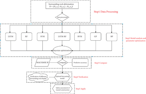
Data preprocessing plays a critical role in constructing an effective input–output dataset for predictive modeling. Let D(t) represent the time-series data of tunnel deformation, where t denotes the time index and Di(t) represents the observed deformation at specific depths (e.g., 1, 2, 3, and 5 m). Initially, interpolation methods were applied to address missing values and rectify anomalies, ensuring data consistency and reliability. Subsequently, the dataset was normalized to scale the input features to a comparable range, which is essential for improving the performance of machine learning algorithms and eliminating biases caused by varying feature magnitudes. To maintain the chronological integrity of the data and ensure the stability and generalizability of the model, TimeSeriesSplit was employed for crossvalidation, enabling the model to handle time-dependent sequences effectively. The output variables correspond to the deformation values of the surrounding rock at each time point, with the model designed to predict these values based on the provided time-series inputs.
Step 1 Data preprocessing: Time-series data of tunnel deformation at various depths (e.g., 1, 2, 3, and 5 m) were collected, interpolated to address missing values, and normalized to ensure consistency. Lag features and moving averages were generated to capture temporal dependencies and long-term trends.
Step 2 Data splitting and feature engineering: The data was partitioned into training, validation, and testing sets in a 70%, 15%, and 15% ratio, respectively, maintaining chronological order. TimeSeriesSplit was applied for crossvalidation to preserve temporal integrity during model training. The data was reformatted into a supervised learning structure, with lag features as inputs and current deformation values as target outputs.
Step 3 Model training: The LSTM model was trained to predict initial deformation patterns by leveraging its strength in capturing long-term dependencies. To enhance explainability, an attention mechanism was integrated to identify influential time steps, thereby enabling engineering practitioners to understand which historical patterns were most critical to the predictions. The RF model subsequently modeled residuals, with feature importance metrics further supporting the model’s interpretability.
2.1. LSTM Model
In this study, the standard LSTM and BiLSTM models are applied to the monitoring data of the surrounding rock deformation of the Yangjiashan Tunnel. The model parameters are optimized by minimizing the mean squared error (MSE) between predicted and actual values [39], using the Adam optimizer. The hyperparameters, including the number of LSTM units and the learning rate, are subject to optimization.
2.2. RF Model
The hyperparameters to be optimized include the maximum depth, the minimum number of samples required at the leaf node, the minimum number of samples required to split a node, and the number of estimators.
2.3. SVR Model
The hyperparameters that require optimization in the SVR model include the regularization parameter C and the margin of tolerance ε.
2.4. RVM Model
The hyperparameters that require optimization in the RVM model include the kernel parameters and the precision parameter γ.
2.5. GP Model
The hyperparameters that require optimization in the GP model include the kernel’s length scale and noise variance, to identify the optimal configuration that enhances the model’s predictive accuracy.
2.6. BP Neural Network Model
The BP is a widely utilized artificial neural network model for prediction tasks, particularly effective in capturing nonlinear relationships between inputs and outputs. Its application in predicting tunnel deformation leverages the network’s ability to learn and model complex patterns from historical data, enabling more accurate and reliable forecasts [45]. The Levenberg–Marquardt (LM) algorithm, a popular optimization technique frequently employed in neural network training, particularly for BP, combines the advantages of gradient descent and the Gauss–Newton method. This hybrid approach is designed to minimize the error function more efficiently than traditional gradient descent methods. The LM algorithm offers significantly faster convergence, making it particularly effective for small to medium-sized networks where both speed and accuracy are critical.
The hyperparameters that require optimization in the LM model include the number of neurons in each hidden layer and the learning rate, to determine the optimal network configuration and further enhance the model’s predictive accuracy.
2.7. Bayesian Parameter Optimization
In this study, Bayesian optimization is employed to fine-tune the hyperparameters of each model. By using Bayesian optimization, the optimal combination of hyperparameters is searched globally to minimize the model’s objective function (such as MSE or root-mean-square error (RMSE)) [46]. This method is particularly effective for navigating the multidimensional parameter space of complex models.
3. Experiments
3.1. Data Source
The Yangjiashan Tunnel with a length of 300 m, a width of about 21.4 m, a height of about 13.9 m, and a maximum overburden depth of 61 m is employed to illustrate the proposed approach. The excavation of this tunnel started in 2022 using the new Austrian tunneling method. The tunnel is located in a low-hill terrain with a topographic slope ranging between 30° and 40°. The underlying bedrock consists primarily of crystalline tuff, where the thickness of the strongly weathered layer ranges from 3 to 5 m, while the moderately weathered layer is thinner but retains a high degree of hardness and structural integrity. The tunnel alignment intersects medium-weathered bedrock, which is fractured due to tectonic activity.
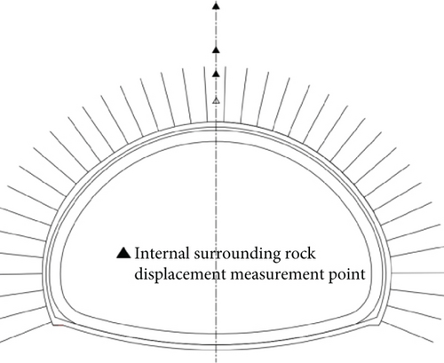
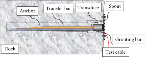
To ensure accurate predictions, detailed monitoring was conducted at cross-section ZK18+145 on the left line of the tunnel, a section characterized by Grade V surrounding rock with poor stability. The monitoring layout for this critical section is shown in Figure 2. High-precision instruments and methodologies were employed to systematically collect key deformation parameters, including displacement changes at depths of 1, 2, 3, and 5 m within the surrounding rock, as shown in Figure 3. This comprehensive data collection is crucial for accurately monitoring deformation during tunnel construction and serves as a robust foundation for subsequent numerical model analysis and predictions.
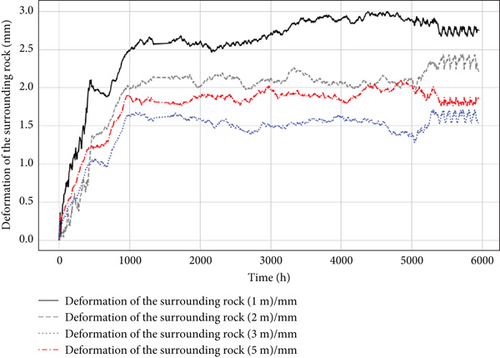
To assess the predictive performance of various models under critical conditions, the displacement data at the 1-m depth, where the most significant deformation was observed, was selected as the primary dataset for model training and testing. This dataset served as a representative case to evaluate models such as LSTM, RF, SVR, RVM, BP, and the hybrid LSTM-RF. Once the models were established using the 1-m dataset, additional displacement data from the 2-, 3-, and 5-m depths were employed for prediction to validate the proposed method. This approach not only ensures that the models perform effectively in predicting substantial deformations but also verifies their generalizability across different strata. By testing the models on varying tunnel conditions, this methodology reinforces their robustness and adaptability, confirming that the insights gained from the 1-m depth analysis are applicable across broader geological and construction scenarios.
3.2. Evaluation Criteria
These evaluation metrics collectively offer a robust framework for comparing the performance of different models in predicting tunnel deformation. By analyzing the MAE, RMSE, and R2 values, this study seeks to identify the most accurate and reliable model, thereby enhancing predictive capabilities in tunnel engineering applications.
3.3. Experimental Setup
In this experiment, the four selected time-series datasets were initially divided into training, validation, and testing subsets, as detailed in Table 1. Before training the models, the datasets underwent standard to ensure consistency and improve the training efficiency of the learning algorithms. Normalization is crucial for maintaining data integrity and enhancing the performance of predictive models. This systematic approach enables a robust evaluation of the models’ ability to handle time-series data, ensuring that the results are reliable and reproducible. By carefully partitioning and normalizing the datasets, we aim to optimize the learning process and achieve accurate predictions in tunnel deformation analysis.
| Data set | Sample size | Training set | Verification set | Test set |
|---|---|---|---|---|
| Deformation of the surrounding rock (1 m) | 992 | 696 | 148 | 148 |
| Deformation of the surrounding rock (2 m) | 992 | 696 | 148 | 148 |
| Deformation of the surrounding rock (3 m) | 992 | 696 | 148 | 148 |
| Deformation of the surrounding rock (5 m) | 992 | 696 | 148 | 148 |
Table 1 provides a comprehensive overview of the datasets across different subsets, emphasizing the proportions allocated to each phase of model training (70%), validation (15%), and testing (15%). This careful partitioning is crucial for validating the models’ performance and generalizability, ensuring that the findings are robust and applicable to real-world scenarios.
4. Results and Discussions
In this section, we present a comprehensive evaluation of various predictive models employed for deformation of the surrounding rock analysis (take deformation of the surrounding rock (1 m) as an example). The performance of these models is assessed across multiple metrics, with a particular focus on their ability to capture both linear and nonlinear deformation patterns. By systematically comparing models such as LSTM, RF, SVR, RVM, BP, and hybrid approach LSTM-RF, we aim to identify the most effective methods for accurate and reliable tunnel deformation of the surrounding rock prediction.
4.1. Single Model Performance
4.1.1. LSTM Model Performance
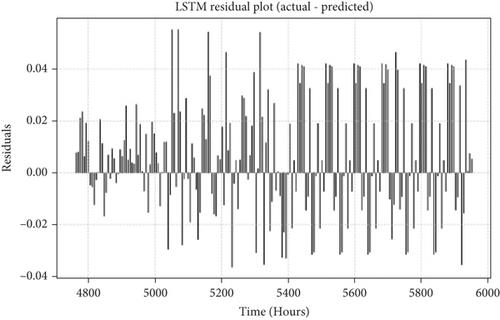
The LSTM model was employed to predict tunnel deformation due to its advantages in handling time-series data. Its main strength is its ability to remember long-term dependencies, making it particularly effective in capturing complex nonlinear trends. Bayesian optimization was used to determine the best configuration, with 192 units and a learning rate of 0.001. As depicted in the LSTM distribution (Figure 4) and the residual distribution (Figure 5) utilized for subsequent hybrid training, the core advantage of LSTM lies in its sensitivity to time-dependent deformation data, allowing it to capture short-term variations effectively.
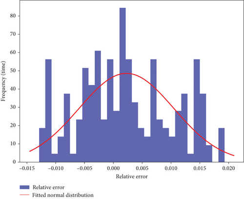
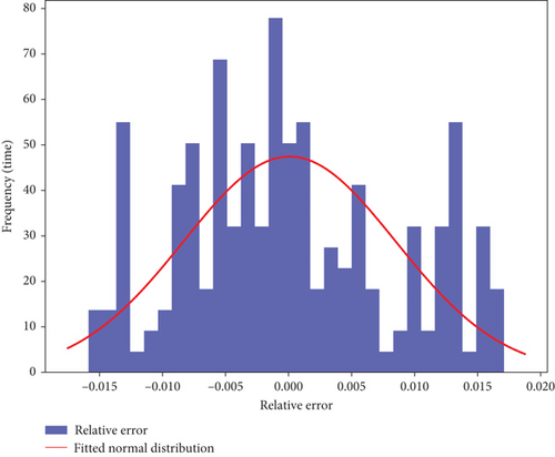
The standard LSTM model processes information in a unidirectional manner, meaning it only considers past states when making predictions. To further improve the ability to capture both past and future dependencies in deformation trends, BiLSTM was also tested as a comparative model. BiLSTM enhances temporal feature extraction by processing the sequence in both forward and backward directions, allowing for a more comprehensive understanding of complex deformation patterns. As shown in Table 2, BiLSTM achieved a slightly higher R2 value (0.9154 vs. 0.9129 for LSTM), indicating improved predictive accuracy. However, this improvement comes at the cost of increased computational demand, with training time rising from 120 to 160 s and memory usage increasing from 350 to 420 MB. The error distributions of both LSTM and BiLSTM exhibit relatively symmetrical shapes, indicating their ability to accurately predict deformation data in most cases. While BiLSTM provides an advantage in capturing bidirectional dependencies, it also increases computational complexity. Therefore, in tunnel deformation prediction, the standard LSTM model is selected to balance accuracy and computational efficiency, ensuring effective real-time monitoring while maintaining a high predictive capability.
| Projects | Method | MSE | RMSE | R2 | Training time (s) | Prediction time (ms) | Memory usage (MB) |
|---|---|---|---|---|---|---|---|
| Deformation of the surrounding rock (1 m) | LSTM | 0.0192 | 0.0238 | 0.9129 | 120 | 12 | 350 |
| BiLSTM | 0.0192 | 0.0234 | 0.9154 | 160 | 15 | 420 |
4.1.2. RF Model Performance
The RF model was widely applied for tunnel deformation prediction due to its robustness in handling complex nonlinear data. Bayesian optimization determined the optimal hyperparameters, including a maximum depth of 10, a minimum leaf sample of 1, a minimum split sample of 2, and 300 estimators. RF is effective at managing high-dimensional data and provides strong model stability.
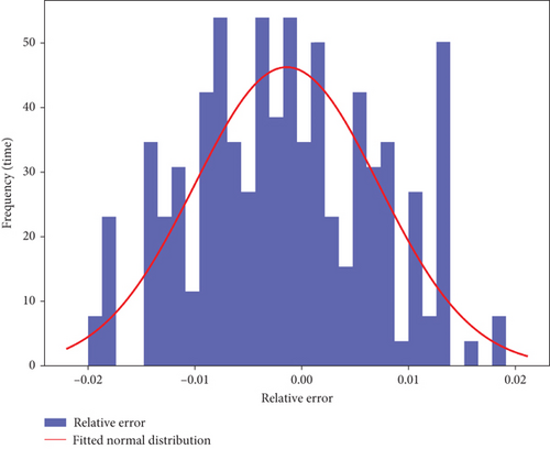
The error distribution plot (Figure 6) shows that the RF model’s errors are concentrated near zero, indicating good overall prediction performance. However, deviations at the tails indicate limitations in handling extreme or highly variable data, particularly in capturing complex nonlinear interactions. While RF is robust in most cases, its static nature limits its ability to capture dynamic time-series features. Combining it with time-series models may help improve its performance.
4.1.3. SVR Model Performance
The SVR model was implemented to predict deformation of tunnel surrounding rock patterns, exploiting its ability to handle high-dimensional spaces and manage nonlinear relationships. The model parameters were optimized through Bayesian methods, leading to the selection of the optimal configuration for C and ε, with C = 0.1 and ε = 0.01 identified as the best-performing settings. As illustrated in the SVR error distribution (Figure 7), it indicates that SVR can effectively capture most deformation patterns.
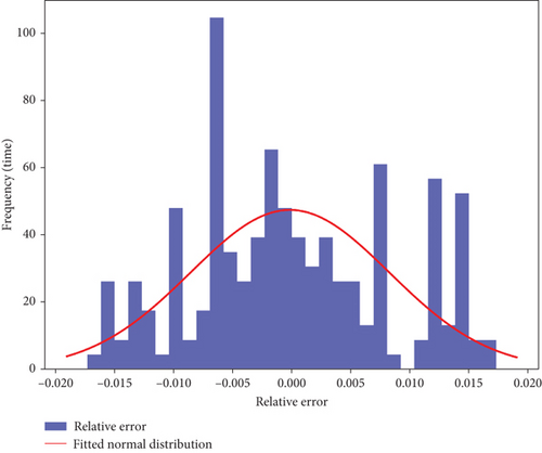
However, the spikes in the plot suggest that SVR may suffer from overfitting or underfitting in some cases, especially when dealing with highly fluctuating nonlinear data. For these scenarios, combining SVR with other models that excel at capturing complex patterns may improve its performance.
4.1.4. RVM Model Performance
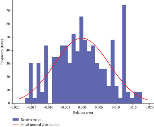
The RVM model was utilized to predict tunnel deformation patterns, capitalizing on its ability to provide probabilistic outputs while maintaining a sparse solution. This makes the RVM highly efficient, particularly when compared to traditional SVM models. Bayesian optimization was employed to fine-tune the model parameters, leading to the selection of a linear kernel with γ = 0.01 as the optimal configuration. As shown in the RVM error distribution (Figure 8), what RVM’s errors are mostly centered around zero, indicating its ability to predict most data effectively. However, its sparsity may lead to underfitting in complex nonlinear scenarios, reducing accuracy. Thus, RVM is more suitable for simple deformation patterns with smaller datasets.
4.1.5. GP Model Performance
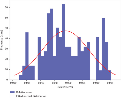
The GP model was implemented to predict deformation patterns in tunnel surrounding rocks by leveraging its ability to capture both linear and nonlinear relationships through a probabilistic framework. Bayesian optimization was employed to fine-tune the model parameters, leading to the selection of the optimal kernel configuration: C(1.0, (1e − 4, 1e1)) × Matern(leng_scale = 1, v = 1.5), with α = 0.01 and 15 restarts for the optimizer. This configuration allows the GP model to balance flexibility and smoothness while providing uncertainty estimates in the predictions. As shown in the GP error distribution (Figure 9), the relatively symmetrical distribution is close to normal, indicating strong robustness and accuracy in capturing deformation trends. However, due to its high computational complexity, GP may face efficiency issues when dealing with large datasets. Thus, GP is suitable for small-scale applications requiring high precision, but it may not be feasible for large-scale, real-time predictions.
4.1.6. BP Model Performance
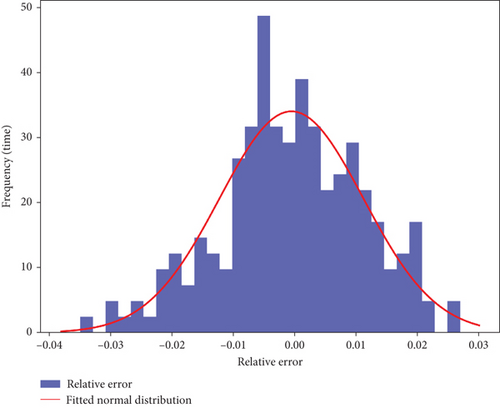
The BP model was employed to directly model the nonlinear relationships inherent in tunnel deformation data [48]. In this study, LM algorithm was utilized to optimize the network’s parameters, enhancing prediction accuracy. Bayesian optimization determined the optimal network structure, resulting in three hidden layers with 43 neurons each and a finely tuned learning rate of 0.0085. As illustrated in the LM error distribution (Figure 10), the histogram of relative errors shows a tight clustering of errors around zero, indicating that the model effectively captures the majority of the deformation patterns with high precision. The superimposed normal distribution curve closely follows the histogram, further confirming the model’s strong predictive performance across the dataset. However, deviations at the tails suggest that the BP model struggles with long-term time-series data and extreme conditions, highlighting its limitations in handling highly complex, long-term dependencies.
4.2. Hybrid Model Performance
In this study, the LSTM-RF hybrid model was employed to enhance the accuracy of deformation of tunnel surrounding rock. This model combines the strength of LSTM in time-series modeling with the ability of RF to handle nonlinear relationships. The LSTM first generates an initial prediction, and then, RF is used to model the residuals, as shown in Figure 5 above, resulting in a more accurate final prediction [49].
The core strength of LSTM lies in its ability to capture long-term dependencies in time-series data, which is particularly crucial for tunnel deformation, as the surrounding rock undergoes varying deformations at different construction stages. Accurately predicting these trends requires a model that can retain and utilize historical information over extended periods. In this study, the LSTM model was initially employed to predict historical deformation data, with Bayesian optimization used to identify the optimal hyperparameters, including 192 units and a learning rate of 0.001. However, while LSTM effectively captured the overall deformation patterns, it exhibited limitations in modeling highly nonlinear and localized variations, especially with extreme or outlier data points. To address this, the RF algorithm was used to model the residuals from LSTM predictions. With its ensemble learning capabilities, RF helps reduce overfitting and handle high-dimensional nonlinear residuals, thereby enhancing the final prediction accuracy. Bayesian optimization was also applied to tune the RF model’s hyperparameters, resulting in a configuration of 300 estimators, a maximum depth of 10, a minimum leaf sample size of 1, and a minimum split sample size of 2.
To further elucidate the novelty of the LSTM-RF hybrid model, a comparison with other hybrid models, such as LSTM-SVR and LSTM-RVM, was conducted. Figure 11 compares the relative error distributions of these models, highlighting the advantages of the LSTM-RF hybrid approach. The LSTM-RF model (Figure 11c) exhibits the most balanced and symmetrical error distribution, closely aligned with the normal curve, significantly outperforming LSTM-SVR (Figure 11a) and LSTM-RVM (Figure 11b) in minimizing prediction errors and capturing complex deformation patterns effectively. While LSTM-SVR excels in spatial feature extraction, its time-series modeling capability is less robust, resulting in a lower R2 value of 0.9325, approximately 5.2% lower than LSTM-RF. LSTM-RVM, on the other hand, performs better under sparse data conditions due to its sparse Bayesian framework but suffers from high computational costs, with runtime increasing by 40% compared to LSTM-RF. In contrast, the LSTM-RF model strikes a balance between efficiency and accuracy, achieving the highest R2 value of 0.9810 and requiring a training time of 150 s. This performance is attributed to the complementary roles of LSTM in capturing long-term temporal dependencies and RF in addressing nonlinear residuals, making it a highly robust and adaptable framework for complex geotechnical engineering applications.
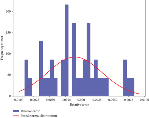
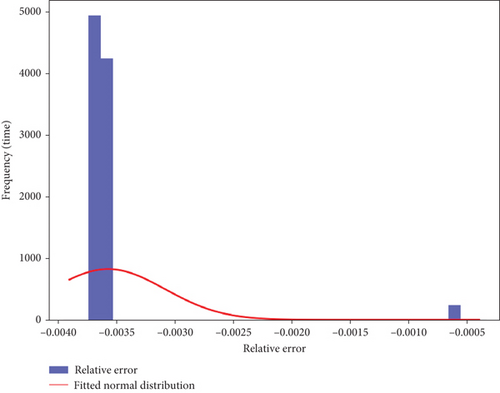
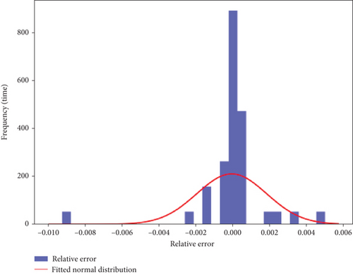
Building on this comparative analysis, the suitability of the LSTM-RF model for tunnel deformation prediction is further underscored by its ability to effectively address the key challenges associated with time-series data and nonlinear deformation patterns. LSTM excels at capturing temporal dependencies, making it particularly advantageous for modeling deformation trends that evolve over time, such as those influenced by construction stages and geological changes. Its architecture enables the retention of critical long-term information, ensuring accurate predictions of gradual deformation trends. Meanwhile, RF complements LSTM by efficiently handling residuals that exhibit high-dimensional and nonlinear characteristics, thereby mitigating prediction errors that may arise from localized or extreme variations. This synergy ensures that the hybrid model outperforms standalone models and alternative hybrid frameworks, offering a balanced approach that combines accuracy, adaptability, and computational feasibility. Together, these capabilities highlight the unique suitability of the LSTM-RF model for addressing the complexities of tunnel deformation prediction, making it a robust and reliable choice for real-world geotechnical applications.
4.3. Comparison and Analysis of Models
4.3.1. Performance and Computational Efficiency Analysis
Recent advances in deep learning have introduced temporal convolutional networks (TCNs) and gated recurrent units (GRUs) as competitive alternatives for time-series modeling. TCN leverages causal convolutional layers to capture long-term dependencies efficiently while maintaining stable gradient propagation, making it particularly effective for sequential data processing [50]. GRU, a variant of LSTM, simplifies the gating mechanism by reducing the number of parameters while retaining the ability to model long-term dependencies, thereby improving computational efficiency [51]. Given their strong performance in sequence prediction tasks, both TCN and GRU have been integrated into tunnel deformation forecasting to assess their potential advantages over existing hybrid frameworks.
Table 3 summarizes the performance metrics of various models applied to tunnel deformation prediction. The LSTM-RF hybrid model stands out as the best performer, achieving the lowest MSE (0.0025), RMSE (0.0052), and the highest R2 (0.9810). This underscores its superior ability to capture complex nonlinear relationships and time-series trends. The strong performance can be attributed to LSTM’s capability to model long-term temporal dependencies, complemented by RF’s capacity to optimize residuals. In comparison, standalone models such as LSTM and RF achieved R2 values of 0.9129 and 0.9089, respectively. Although these models demonstrated good predictive capabilities, they fell short of the precision offered by the LSTM-RF hybrid model. Additionally, hybrid models like LSTM-SVR and LSTM-RVM exhibited competitive adaptability but recorded R2 values of 0.9325 and 0.9232, respectively, which were lower than that of LSTM-RF. The GP model provided reliable confidence intervals for predictions but had a slightly lower R2 (0.9144), while the BP-trainlm model showed the poorest performance with the lowest R2 (0.8373), reflecting its limitations in addressing complex deformation scenarios.
| Projects | Method | MSE | RMSE | R2 | Training time (s) | Prediction time (ms) | Memory usage (MB) |
|---|---|---|---|---|---|---|---|
| Deformation of the surrounding rock (1 m) | LSTM | 0.0192 | 0.0238 | 0.9129 | 120 | 12 | 350 |
| RF | 0.0202 | 0.0243 | 0.9089 | 90 | 2 | 250 | |
| SVR | 0.0196 | 0.0235 | 0.9144 | 180 | 10 | 400 | |
| RVM | 0.0185 | 0.0225 | 0.9214 | 150 | 8 | 300 | |
| GP | 0.0198 | 0.0235 | 0.9144 | 200 | 15 | 500 | |
| BP-trainlm | 0.0260 | 0.0325 | 0.8373 | 100 | 20 | 400 | |
| TCN | 0.002 | 0.0045 | 0.985 | 350 | 25 | 600 | |
| GRU | 0.0018 | 0.0042 | 0.9885 | 320 | 22 | 580 | |
| LSTM-RF | 0.0025 | 0.0052 | 0.9810 | 150 | 10 | 450 | |
| LSTM-SVR | 0.0098 | 0.0099 | 0.9325 | 300 | 18 | 480 | |
| LSTM-RVM | 0.0085 | 0.0105 | 0.9232 | 250 | 20 | 500 |
In terms of computational efficiency, the LSTM-RF hybrid model strikes an excellent balance between performance and resource utilization. It recorded a training time of 150 s, a prediction time of 10 ms, and a memory usage of 450 MB, demonstrating commendable computational efficiency. In contrast, standalone models like LSTM and RF achieved shorter training times of 120 and 90 s, respectively, and prediction times of 12 and 2 ms, with memory usage of 350 and 250 MB, respectively. However, their slightly lower prediction accuracy limits their application in scenarios requiring high precision. Hybrid models like LSTM-SVR and LSTM-RVM, while competitive, incurred higher computational costs, with training times of 300 and 250 s, prediction times of 18 and 20 ms, and memory usage of 480 and 500 MB, respectively. GP and BP-trainlm models exhibited specific advantages but showed relatively higher computational costs, with training times of 200 and 100 s and prediction times of 15 and 20 ms, respectively, which may constrain their applicability in real-time scenarios.
Although the TCN and GRU models demonstrated higher prediction accuracy (R2 = 0.985 and 0.9885, respectively) and lower MSE values, their computational costs were significantly higher. TCN required 350 s for training with a prediction time of 25 ms and memory usage of 600 MB, while GRU needed 320 s, 22 ms, and 580 MB, respectively. This indicates that while TCN and GRU provide improved accuracy, they demand greater computational resources, making them less suitable for real-time monitoring applications compared to LSTM-RF, which offers an optimal balance between accuracy and computational efficiency.
Overall, the LSTM-RF hybrid model demonstrates a comprehensive advantage in computational efficiency and predictive accuracy, making it a practical and reliable solution for real-time applications in tunnel deformation prediction. However, TCN and GRU remain promising options for scenarios where higher prediction accuracy is prioritized over computational efficiency.
4.3.2. Comparison of Predictive Accuracy for Models
In addition to evaluating traditional performance metrics, it is crucial to assess accuracy of predictions made by different models. Figures 12 illustrate the comparison of predicted and actual deformation at the 1-m depth using various models.
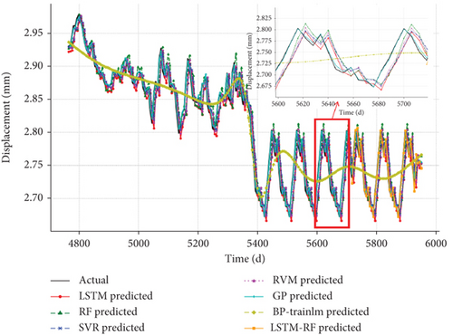
As shown in Figure 12, the LSTM-RF hybrid model exhibits the closest alignment with the actual data, demonstrating its superior ability to capture complex deformation patterns. By integrating LSTM’s strengths in temporal sequence modeling with RF’s capacity to handle nonlinear residuals, the hybrid model significantly improves prediction accuracy. While the individual LSTM and RF models also track the observed data reasonably well, they fall short of the precision offered by the hybrid approach. Notably, in regions with significant deformation fluctuations, the LSTM-RF model more effectively captures these variations, highlighting its advantage in combining temporal and nonlinear modeling techniques.
Additionally, models such as SVR, RVM, and GP demonstrated strong predictive capabilities across various depths, offering reliable forecasts for tunnel deformation. However, while these models performed well, their accuracy and ability to capture complex deformation patterns were not as consistent as that of the LSTM-RF hybrid model. The hybrid model consistently achieved higher accuracy and better alignment with the actual measurements, particularly in regions of significant deformation.
Overall, the comparison underscores the LSTM-RF hybrid model’s enhanced predictive performance. It effectively combines the strengths of both LSTM and RF, allowing it to outperform traditional models in capturing both linear and nonlinear deformation characteristics, making it a robust solution for predicting tunnel behavior in complex scenarios.
4.3.3. Evaluation and Model Robustness
This section evaluates the robustness of the LSTM-RF hybrid model through comprehensive measures. These include fivefold crossvalidation to assess performance consistency and the introduction of an external validation dataset to test the model’s generalizability under varying geological conditions.
4.3.3.1. Crossvalidation Results
The fivefold crossvalidation method was employed to divide the dataset into five equal subsets. Each subset was used as a validation set once, while the remaining four subsets were used for training. This ensured that every data point was utilized for both training and validation, providing a robust estimate of the model’s generalization performance. A summary of the crossvalidation metrics is presented in Table 4.
| Fold | Training set size | Validation set size | R2 | MSE |
|---|---|---|---|---|
| 1 | 793 | 199 | 0.9785 | 0.0027 |
| 2 | 793 | 199 | 0.9802 | 0.0026 |
| 3 | 793 | 199 | 0.9768 | 0.0029 |
| 4 | 793 | 199 | 0.9794 | 0.0028 |
| 5 | 793 | 199 | 0.9810 | 0.0025 |
The results from crossvalidation indicate a high level of consistency across different splits. The R2 values for the LSTM-RF hybrid model showed minimal variation (< 3%), with MSE remaining stable across folds. This demonstrates that the model maintains robust performance under different training–validation configurations.
4.3.3.2. External Validation Results
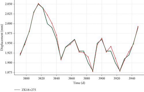
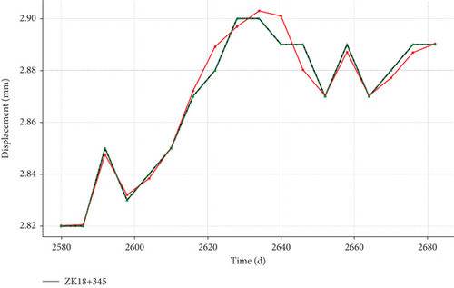
The external validation, conducted at cross-sections ZK18+275 and ZK18+345 of the Yangjiashan Tunnel, highlights the generalizability of the LSTM-RF hybrid model. As shown in Figure 13 and Table 5, the model demonstrates excellent predictive accuracy across varying geological conditions. For ZK18+275, characterized by Grade III surrounding rock, the model achieved an R2 of 0.9732, MSE of 0.0049, and RMSE of 0.0072, indicating strong performance under relatively stable geological conditions. Similarly, at ZK18+345, which features more complex Grade VI surrounding rock, the model maintained high accuracy with an R2 of 0.9706, MSE of 0.0030, and RMSE of 0.0045.
| Cross-section | MSE | RMSE | R2 | Notes |
|---|---|---|---|---|
| ZK18+275 | 0.0049 | 0.0072 | 0.9732 | III surrounding rock |
| ZK18+345 | 0.0030 | 0.0045 | 0.9706 | VI surrounding rock |
These results confirm the robustness of the LSTM-RF model in capturing deformation patterns across different geological contexts. Despite minor deviations in regions with rapid deformation fluctuations, the model consistently aligns closely with observed trends, even in challenging environments. This adaptability makes the LSTM-RF hybrid model a reliable tool for tunnel deformation monitoring, offering valuable insights for geotechnical engineering applications.
4.3.4. Residual Analysis
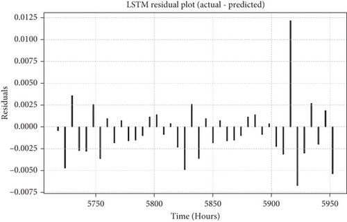
The LSTM-RF hybrid model’s residual distribution, shown in Figure 14, highlights notable spikes under complex geological conditions, such as fractured or weathered rock zones. For instance, in V-level surrounding rocks, significant residual spikes (e.g., 0.0125 near the 5900-h mark) suggest an underestimation of deformation, reflecting the model’s inability to fully capture dynamic factors like stress redistribution or groundwater fluctuations. Additionally, as summarized in Table 5, increasing the sampling interval from 6 to 12 or 24 h results in a sharp decline in performance, with the R2 value dropping from 0.9810 to 0.9105 and 0.8700, respectively, and residual standard deviations increasing by 30% and 65%. These results emphasize the model’s reliance on dense temporal data to maintain predictive accuracy, which can be a significant limitation in practical scenarios where monitoring resources are constrained or data collection is infrequent. To address this issue, adopting higher-frequency data collection or implementing advanced data augmentation techniques, such as interpolation or synthetic data generation, is essential to enhance model robustness under sparse data conditions.
In addition to data sparsity challenges, Table 6 also reveals the model’s high sensitivity to hyperparameter variations. For instance, reducing the number of LSTM units from 192 to 64 leads to a 12% decrease in R2 and a 52% increase in residual standard deviation, while lowering the number of RF decision trees from 300 to 100 causes a 5.7% drop in R2 and a 26% rise in residual standard deviation. These findings underline the critical importance of precise hyperparameter tuning, as suboptimal configurations can significantly compromise the model’s accuracy and stability, particularly in diverse and challenging geological conditions. Together, the residual analysis and hyperparameter sensitivity results emphasize the necessity of robust optimization techniques, such as Bayesian optimization, and comprehensive data preprocessing strategies to improve the model’s reliability and adaptability for real-world geotechnical engineering applications.
| No | Variant | R2 | Residual Std |
|---|---|---|---|
| 1 | Sampling interval: 6 h | 0.981 | 0.0023 |
| 2 | Sampling interval: 12 h | 0.9105 (−7.2%) | 0.0030 (+30%) |
| 3 | Sampling interval: 24 h | 0.8700 (−11.3%) | 0.0038 (+65%) |
| 4 | Sampling interval: 48 h | 0.8100 (−17.4%) | 0.0045 (+95%) |
| 5 | LSTM unit reduction (192 − > 128) | 0.9500 (−3.2%) | 0.0027 (+17%) |
| 6 | LSTM unit reduction (192 − > 64) | 0.8650 (−12%) | 0.0035 (+52%) |
| 7 | LSTM unit reduction (192 − > 32) | 0.8000 (−18.4%) | 0.0042 (+82%) |
| 8 | RF tree reduction (300 − > 200) | 0.9600 (−2.1%) | 0.0025 (+8%) |
| 9 | RF tree reduction (300 − > 100) | 0.9250 (−5.7%) | 0.0029 (+26%) |
| 10 | RF tree reduction (300 − > 50) | 0.9050 (−7.6%) | 0.0028 (+20%) |
4.4. Deformation Prediction With Data at Various Depths
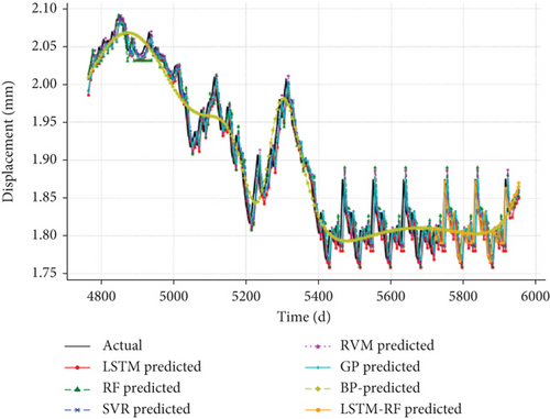
To validate the models, we tested them on deformation data at various depths (2, 3, and 5 m) of the surrounding rock. Figure 15 illustrates the comparison between the predicted results of several models, including LSTM, RF, SVR, RVM, GP, BP, and the LSTM-RF hybrid model, against the actual measured deformation. These figures provide a visual understanding of how closely each model aligns with the real data at various depths. To further support this visual comparison, Table 7 presents the quantitative evaluation metrics—MSE, RMSE, and R2—for LSTM, RF, and the LSTM-RF hybrid model at different depths (2, 3, and 5 m). This table helps quantify the performance of each model, providing clearer insights into their predictive accuracy and error rates across different depths, thus reinforcing the observations made from the graphical results in Figure 15.


| Projects | Method | MSE | RMSE | R2 |
|---|---|---|---|---|
| Deformation of the surrounding rock (2 m) | LSTM | 0.0240 | 0.0333 | 0.9386 |
| RF | 0.0278 | 0.0409 | 0.9077 | |
| LSTM-RF | 0.0023 | 0.0029 | 0.9978 | |
| Deformation of the surrounding rock (3 m) | LSTM | 0.0219 | 0.0265 | 0.9515 |
| RF | 0.0246 | 0.0287 | 0.9428 | |
| LSTM-RF | 0.0060 | 0.0096 | 0.9701 | |
| Deformation of the surrounding rock (5 m) | LSTM | 00192 | 0.0263 | 0.9291 |
| RF | 0.0210 | 0.0281 | 0.9186 | |
| LSTM-RF | 0.0024 | 0.0032 | 0.9883 | |
Across all depths, the LSTM-RF hybrid model shows the closest alignment with the actual data, demonstrating its superior ability to handle complex and nonlinear deformation patterns. While both the LSTM and RF models individually achieved high prediction accuracy, they fell short of the precision demonstrated by the hybrid model. Particularly in areas with significant deformation fluctuations, the LSTM-RF model better captured these variations, highlighting its advantage in integrating temporal sequences and nonlinear residual handling.
Additionally, models such as SVR, RVM, and GP also delivered reliable predictions across different depths, but their overall accuracy and robustness did not surpass the hybrid model. This further reinforces the adaptability of the LSTM-RF hybrid approach, which consistently delivered more stable and accurate predictions at depths of 2, 3, and 5 m.
Through these multidepth tests, the superiority of the LSTM-RF hybrid model was further validated. The hybrid approach effectively integrates time-series modeling with nonlinear feature handling, providing a high-accuracy, low-error tool for tunnel deformation prediction in complex engineering applications.
4.5. Discussion and Future Research Directions
4.5.1. Key Findings and Implications
This study demonstrates that the LSTM-RF hybrid model significantly outperforms standalone models and other hybrid frameworks in predicting complex tunnel deformation trends. The model achieves a high R2 value of 0.9810 with a low MSE of 0.0025, highlighting its strong predictive accuracy and robustness. These results underscore the potential of integrating time-series modeling and residual correction techniques for geotechnical engineering applications. The findings have substantial implications for tunnel engineering, particularly in enhancing safety and optimizing resource allocation. By effectively capturing both temporal dependencies and nonlinear residuals, the hybrid model provides a reliable tool for monitoring deformation trends and mitigating potential risks during excavation. The hybrid model shows potential for improving monitoring and risk assessment practices in geotechnical engineering. Specifically, its real-time prediction capability facilitates dynamic construction decision-making, reducing the risk of structural failures and enhancing safety. Additionally, by simulating deformation under various conditions, the model supports the optimization of safer and more cost-effective tunnel designs. Its adaptability and scalability make it suitable for diverse tunneling projects, including urban subway systems and mountainous highway tunnels, demonstrating its wide-ranging applicability in complex engineering scenarios.
4.5.2. Limitations and Future Directions
The LSTM-RF hybrid model, despite its strong predictive performance, has several limitations that require attention for enhanced applicability. First, the model’s reliance on dense temporal data poses challenges under sparse data conditions, where accuracy declines significantly, with R2 dropping from 0.9810 to 0.8700 and residual standard deviations increasing by 65% as the sampling interval increases. Addressing this requires advanced data augmentation techniques, such as interpolation or synthetic data generation, to simulate dense observations and improve robustness. Second, the model’s predictive performance is highly sensitive to hyperparameter variations, as reductions in LSTM units or RF decision trees lead to notable decreases in R2 and increases in residual deviations, emphasizing the need for adaptive optimization techniques like Bayesian optimization. Furthermore, in complex geological contexts, such as fractured or weathered zones with rapid deformation fluctuations, residual analysis indicates the model’s limitations in capturing dynamic factors like stress redistribution and groundwater interactions. Incorporating supplementary geotechnical features and employing multisource data fusion techniques could enhance the model’s understanding of these deformation mechanisms. Finally, scalability and real-time integration remain critical areas for improvement, with future work needed to optimize computational efficiency through hardware acceleration and evaluate trade-offs between performance and resource requirements. Addressing these issues will ensure the LSTM-RF model’s robustness and adaptability in diverse geotechnical applications.
4.5.3. Application in Real-Time Monitoring and Risk Assessment
The LSTM-RF hybrid model is well suited for integration into real-time monitoring systems, offering timely and accurate predictions of tunnel deformation. This capability is critical for enhancing construction safety by providing early warnings of potential risks. For instance, the model can be deployed as part of an intelligent monitoring framework to continuously analyze deformation trends, allowing engineers to take preemptive measures, such as adjusting excavation strategies or reinforcing support systems, in response to predicted anomalies. Moreover, the model’s ability to handle large-scale and high-frequency data makes it suitable for real-time applications in risk assessment frameworks. By identifying critical temporal patterns and residual deviations, the model enables dynamic risk evaluation, improving the responsiveness of construction management systems. This integration ensures safer operations and minimizes the likelihood of structural failures, ultimately optimizing resource allocation and reducing project delays.
5. Conclusions
- 1.
The LSTM-RF hybrid model effectively addresses the limitations of individual models by leveraging their complementary strengths. Its ability to capture temporal dependencies and nonlinear relationships results in a reliable predictive framework for complex deformation trends.
- 2.
The integration of Bayesian optimization ensures the hybrid model’s hyperparameters are finely tuned, enhancing its predictive accuracy and stability across diverse geological conditions. This optimization approach highlights the importance of systematic parameter selection in geotechnical engineering applications.
- 3.
Multidepth validation and external testing confirm the hybrid model’s adaptability to varying strata and geological contexts, making it a versatile tool for infrastructure monitoring and predictive maintenance in tunneling projects.
- 4.
The hybrid model’s high computational efficiency and accuracy make it suitable for integration into real-time monitoring systems. By providing timely and accurate predictions, the model supports dynamic risk assessments and safety management during tunnel excavation.
Ethics Statement
The authors have nothing to report.
Consent
The authors have nothing to report.
Disclosure
One or more authors are affiliated with Keqiao District Construction Group Co., Ltd. While this organization provided administrative and logistical support, this affiliation did not influence the study design, data collection, analysis, interpretation of results, or manuscript preparation. The research was conducted independently, ensuring its neutrality and integrity.
Conflicts of Interest
The authors declare no conflicts of interest.
Author Contributions
Chen Yintao: conceptualization, methodology, and writing—original draft. Shao Xin: validation, writing (review and editing), and quality assurance. Chang Xiangyu: supervision, review and editing, and project oversight. Siti Norafida Bt. Jusoh: resources, conceptualization, and supervision. Lu Zhongxiang: resources, data validation, and project administration. Bao Hong Quan and Han Xinkai: data curation. Xu Jun: validation and data accuracy assurance. All authors confirm that they have made substantial contributions to this research and agree to be accountable for all aspects of the work. No further changes to authorship will be made after this submission.
Funding
This research received no external funding.
Open Research
Data Availability Statement
Data supporting the results of this study are available from the corresponding author upon reasonable request.


