In this work, we formulate and examine a mathematical model of cigarette smoking dynamics with optimal control theory. Firstly, we demonstrated that the solution of the model is a bounded region and nonnegative, which demonstrated that the model is well posed both mathematically and epidemiologically. Besides, we computed the cigarette smoking–free equilibrium and the endemic equilibrium points of the model. Then, the basic reproduction number was computed using the next-generation matrix, and the stability analysis of the equilibrium points was examined. The analysis shows that the cigarette smoking–free equilibrium point is stable over time if the basic reproduction number is less than one; otherwise, the model will reach the endemic equilibrium point. Also, a sensitivity analysis was conducted to assess the impact of key factors on cigarette smoking dynamics. Moreover, we extended the cigarette smoking dynamics model to an optimal control model via two controls: educating individuals and treating addicted smokers. Then, the existence of optimal controls is proven, and using Pontryagin’s minimum principle, the essential conditions of the optimal control model are examined. Also, if the resource is limited, a cost-effectiveness analysis is considered to identify the least costly strategies. Finally, the numerical simulation of optimality systems concluded that educating individuals to keep them away from the smoking addiction population is the most effective strategy to lessen the addiction of cigarette smoking.

1. Introduction

The act of smoking involves burning a cigarette and inhaling the smoke through your mouth, inhaling it into your lungs through pipes, and then letting it out. Numerous dangerous particles are present in cigarette smoke, and when smoking cigarettes, these particles can enter the body and cause harm [1]. Cigarette smoking is linked to several factors, such as age, peer pressure, peer smoking, parental smoking, parental socioeconomic status, family and friend attitudes, school-related issues, risky behaviors, lifestyle, stress, self-esteem, attitudes, and health concerns [2]. The study in [3] indicates that cigarette smoking is the primary cause of lung cancer. The most common cause of cancer-related deaths is lung cancer. So, 85% of lung cancer deaths are related to cigarette smoking. Smoking affects almost every organ in the body and causes several disorders. Approximately 6 million people die from cigarette smoking every year. Out of them, over 5 million people smoke, and over half do not smoke. According to the World Health Organization (WHO) report on the worldwide cigarette smoking epidemic, cigarette smoking–related deaths are rising annually. The tobacco industry has experienced significant expansion in recent decades, despite declining smoking rates in high-income countries. This growth has been driven by growing smoking in developing regions [4].

In epidemiology, mathematical modeling has proven to be a useful tool for comprehending and characterizing the dynamics of infectious illness [5]. Numerous mathematical studies have been carried out to better understand the reasons behind and strategies for preventing cigarette smoking around the world to decrease the number of both occasional and habitual smokers [6, 7]. For example, Castillo et al. [8] proposed the mathematical models for the dynamics of tobacco. The authors suggest that counseling efforts, or cultural immunization, create a class of individuals less likely to relapse and by no means susceptible. Sharomi and Gumel [9] developed a mathematical model of tobacco smoking dynamics and extended the work in [8] by adding a group of smokers who had temporarily stopped. The authors suggest that, regardless of how long mild smokers stayed in their class, the number of smokers in the community will be drastically decreased if chain smokers do not continue to smoke. Zaman [10] proposed a mathematical model for giving up smoking. According to their research, the strategy proposed will work with epidemic models other than the quitting smoking model. Lahrouz et al. [11] studied a deterministic mathematical model for smoking and extended it to a stochastic model by incorporating random noise. According to the authors, the size of the noise intensities and the model system’s parameters determine the stochastic stability of the current smoking equilibrium state. Fekede and Mebrate [12] proposed a mathematical model of secondhand smoking tobacco. The authors suggest that if the average number of smokers that a single addicted smoker produces is less than one, the population of secondhand smokers disappears over time; otherwise, the population of secondhand smokers persists.

Optimal control theory is a powerful mechanism that offers several efficient management ways to reduce or eliminate a community infection [13–15]. Several authors investigated an optimal control model to describe the role of control interventions on smoking dynamics. For example, Sun and Jia [16] developed optimal control of a delayed smoking model with immigration using two measures that control education campaigns and media campaigns for susceptible individuals and heavy smokers, respectively. Their study reveals that the combination of both is the best strategy for the elimination of susceptible individuals and heavy smokers. Nur [17] developed a mathematical modeling of the dynamics of smoking that includes optimum control interventions. The impact of control initiatives, such as treatment and prevention programs, on the dynamics of cigarette smoking in a community is then ascertained by the application of optimum control analysis. According to the study’s control, there is a rise in the population’s number of individual ex-smokers and a fall in the number of potential and current smokers. Omaret and Allali [18] developed an optimal control model by incorporating two control variables, namely, the government’s restriction on smoking in public places, while the second control represents the cost of cigarettes rising and an education campaign. The findings validate that the crucial function of control measures in diminishing the quantity of sporadic and habitual smokers potentially spares a noteworthy number of lives within the smoking community. Moreover, Liuyong et al. [19] presented the cigarette smoking dynamics with optimal control and analysis of cost-effectiveness. In their conclusion, the best, optimal, and least cost-effective controls to prevent tobacco use are the combination of media coverage and smoking cessation treatment.

However, all of these researchers did not consider an optimal control model via two controls: educating individuals and treating addicted smokers with cost-effective strategies. Hence, to fill this gap, we extended the cigarette smoking dynamics model in [9] to an optimal control model via two controls: educating individuals and treatment of addicted smokers. Besides, if the resource is limited, we considered a cost-effectiveness analysis to identify the most optimal and least costly strategies.

The remaining part is summarized as follows: The mathematical model framework for the spread of cigarette smoking is presented in Section 2. The stability of the endemic and cigarette smoking–free equilibria, as well as the positivity and boundedness of solutions, are examined in Section 3. The optimal control model for cigarette smoking dynamics is carried out analytically in Section 4 using the Pontryagin minimum principle. The topic of numerical simulation is covered in Section 5. Section 6 concludes with a statement.

2. Model Formulation

In this section, we investigate a mathematical modeling of the dynamics of cigarette smoking addiction using the NSAR (susceptible, smoker, addicted, and recovered) deterministic model [9]. To illustrate the addiction to smoking cigarettes, the entire population T(t) is separated into four compartments: nonsmoker compartment (susceptible individuals) N(t), cigarette smoker compartment S(t), cigarette smoking addicted A(t), and recovered R(t). In order to control the mathematical model of smoking cigarette addiction dynamics, this model is guided by the following assumptions:

1.
Total population is assumed constant. Hence, migration and immigration factors are ignored.
2.
Population is mixing homogenously.
3.
Newborns are assumed to be susceptible.
4.
Recovered individuals are not permanently immune.

At a rate of π, the susceptible individuals are entering the population. The susceptible individuals become smokers either by smokers or addicted individuals with a force of infection β(S + τA), where β is the transmission rate and τ is the coefficient of transmission for the addiction to cigarette smoking. The addicted are more likely to infect others than smokers if τ > 1. Both smokers and addicts have an identical chance of infecting the susceptible if τ = 1; however, if τ < 1, smokers are more likely to infect the susceptible than addicts. Individual smokers progress at a rate of α to the addicted compartment with a probability of ρ, while the remaining individuals move to the recovery compartment with a probability of 1 − ρ via education or therapy. In other words, a population model of smoking dynamics must take into account the fact that millions of individuals die each year from smoking-related illnesses [2]. It is assumed that, in the addicted compartment, they have a higher probability of developing smoking-related illnesses in comparison to those in the smoker compartment. Addicted individuals move to either the recovered compartment at a rate of γ through education and/or treatment or pass away from their addiction at a rate of δ. The recovered people revert to susceptibility to smoking cigarettes at a rate of η. The natural death rate of individuals in each compartment is μ, and all the parameters are positive.

The flow of people from one compartment to the next is shown in Figure 1, and it can be written into a system of differential equations as follows.

()

with initial conditions: N(0) = N₀ > 0, S(0) = S₀ ≥ 0, A(0) = A₀ ≥ 0, and R(0) = R₀ ≥ 0.

Details are in the caption following the image — **Figure 1**
Open in figure viewer PowerPoint

Flow chart of the model.

3. Model Analysis

In this section, we investigate the invariant region, positivity of the solution, disease-free equilibrium point, basic reproduction number, endemic equilibrium point, and local and global stability of equilibrium points of the system (1).

3.1. Invariant Region

To solve the cigarette smoking dynamics model (1), the invariant region must be biologically meaningful and mathematically well-posed, resulting in a bounded solution.

Theorem 1. The positively feasible set for system (1) is the closed region

Proof 1. We need to replace all of system (1)’s state equations and differentiate the population as a whole with regard to time in order to validate the theorem. The following outcomes emerge from this:

()

If there is no death due to cigarette smoking, then Equation (2) is reduced to . Resolving using the starting condition, we obtain

()

Evaluating Equation (3) as t⟶∞, we get T(t) ≤ π/μ, which implies that 0 ≤ T(t) ≤ π/μ. Hence, the feasible region of system (1) is

()

3.2. Positivity of the Solutions

In this subsection, we are going to show that all solutions of cigarette smoking dynamics model (1) with nonnegative initial data will remain nonnegative for all time t ≥ 0.

Theorem 2. For all future times, all of the solution sets N(t), S(t), A(t), and R(t) are nonnegative if N₀ > 0, S₀ ≥ 0, A₀ ≥ 0, and R₀ ≥ 0.

Proof 2. Let us use the first equation from system (1) in order to demonstrate this theorem:

This equation can be expressed without loss of generality, after eliminating the positive term (π + ηR), as an inequality

()

Then, solving Equation (5) using separation of variables, we get

()

Using the initial conditions, Equation (6) becomes

()

Given that the exponential function can never be negative, e^{−∫[β(S + τA) + μ]dt} is a number that is not negative. Therefore, we can say that N(t) ≥ 0. Similar to this, we get

()

Equations (7) and (8) show that system (1) solution is nonnegative for any t ≥ 0. Thus, the region Ω in Equation (4) contains all of system (1)’s feasible solutions. As a result, the model has mathematical well-posedness and epidemiological significance.

3.3. Cigarette Smoking–Free Equilibrium

Free equilibrium points for cigarette smoking addiction are steady-state situations in which addiction to cigarette smoking does not exist. It is obtained by setting the cigarette smoker state variable S = A = 0 and equating the entire right-hand side of system (1) to zero and solving them. As a result, Ξ₀, the cigarette smoking addiction–free equilibrium of system (1), is given by

()

3.4. The Basic Reproductive Number

The average number of secondary instances that could result from the introduction of one sick person into a completely sensitive society is known as the basic reproduction number (R₀) [20]. Inferring from the sociological definition R₀ in [21], we can redefine our R₀ in the context of this study as follows: R₀ is the average number of secondary smokers caused by a single smoker person during his/her entire smoker period in a completely susceptible population. It can be obtained using the next-generation matrix technique outlined in [22, 23]. The first step is to rewrite system (1), starting with the class that was just a smoker.

()

Then, from system (10), the new cigarette smoker terms and the remaining are transition terms given by the matrices

and

, respectively:

()

The Jacobian matrices of Equation (11) at equilibrium point where cigarette smoking addiction is absent are as follows:

()

From Equation (12), the matrix

at Ξ₀ is invertible and hence

()

Using the next-generation matrix, from Equations (12) and (13), we get

()

As a result, from Equation (14), the

can be found as follows:

()

The average number of secondary cases that one main case in a fully vulnerable population generates is known as the basic reproduction number of cigarette smoking addiction. Hence, the first term gives the number of secondary infections produced by one smoker, and the second term gives the number of secondary infections produced by one addicted individual.

3.5. Stability Analysis of Cigarette Smoking–Free Equilibrium

Theorem 3. The cigarette smoking–free equilibrium point is locally asymptotically stable if and otherwise unstable.

Proof 3. We investigate the cigarette smoking addiction–free equilibrium points’ local stability using the Jacobean matrix. Using Equation (9), the Jacobian matrix of system (1) is

Expanding the determinant of by the first and last columns yields two eigenvalues of : λ₁ = −μ < 0 and λ₂ = −(η + μ) < 0. The last two eigenvalues are the eigenvalues of the next matrix:

()

The cigarette smoking addiction–free equilibrium point of system (1) is locally asymptotically stable if and . That is, from Equation (16), we have

()

Hence, from Equations (17) and (18), we have and if . Therefore, Ξ₀ is locally asymptotically stable.

Theorem 4. If , system (1)’s equilibrium free from addiction to smoking cigarettes is globally asymptotically stable; if , it is unstable.

Proof 4. In order to demonstrate the smoking-free equilibrium point’s global stability, we build the Lyapunov function as L = c₁S + c₂A, where arbitrary constants are used. Then, differentiating with respect to time gives

()

Substituting the values of S^′(t) and A^′(t) from system (1) into Equation (19), we obtain

()

Putting c₂ = −((βN − (α + μ))/ρα)c₁. Then, from Equation (20), we get

()

Taking c₁ = 1, then Equation (21) becomes

Thus, the trajectory of system (1) on which dL/dt = 0 if and only if A = 0, and dL/dt ≤ 0 for . This suggests that at Ξ₀, the only dL/dt ≤ 0. According to Lasalle’s invariance principle, Ξ₀ is thus globally asymptotically stable in Ω [24–26]. The fact that cigarette smoking is currently globally asymptotically stable indicates that a substantial and long-lasting decline in smoking rates throughout a population can be anticipated with the implementation of successful public health initiatives.

3.6. Endemic Equilibrium and Its Stability Analysis

The endemic equilibrium point, represented by Ξ^∗ = (N^∗, S^∗, A^∗, R^∗), exists when cigarette smoking is present in the population. By solving for the state variables and setting all of the model’s Equation (1) to zero, we may obtain

()

Considering that (γ + δ + μ)(η + μ)² is a strong positive term, (1 − ρ)α(γ + δ + μ) and γρα are comparatively smaller negative and positive terms, respectively. The denominator is positive because the strong positive factor dominates the impact of the smaller positive and negative terms taken together. The endemic equilibrium point expression’s denominator is therefore positive for appropriate parameter values and the common presumption that .

Theorem 5. For system (1), the endemic equilibrium point at Ξ^∗ is locally asymptotically stable if .

Proof 5. To show the local stability of the endemic equilibrium point of system (1), we use the linearization approach. Thus, the Jacobian matrix becomes at the endemic equilibrium point

()

Additionally, at the endemic equilibrium point, the characteristic equation of the Jacobian matrix (Equation (23)) is provided by the following:

()

where

All roots of characteristic polynomials (Equation (24)) contain negative real portions according to the Routh–Hurwitz criterion if and only if Ψ₁ > 0, Ψ₂ > 0, Ψ₃ > 0, Ψ₄ > 0 and for the basic reproduction number in Equation (15) is greater than unity. Because of this, the endemic equilibrium is asymptotically stable locally.

Next, we want to demonstrate the globally asymptotically stable endemic equilibrium of the NSAR model. Combining the classical method of Lyapunov functions with Volterra–Lyapunov matrix features [27] can demonstrate global stability. First, we introduce relevant concepts and notations that will facilitate our global stability analysis [28].

Lemma 1 ([27, 29]). If there exists a positive diagonal matrix D_n×n > 0 such that DA + A^tD^t < 0 then A_n×n is Volterra–Lyapunov stable.

Lemma 2 ([27, 29]). If there exists the diagonal matrix D_n×n > 0 such that DA + A^tD^t > 0 then A_n×n is diagonally stable.

Proposition 1 ([27, 29]). The is Volterra–Lyapunov stable if and only if: a₁₁ < 0, a₂₂ < 0 and det(A) > 0.

Proposition 2 ([27, 29]). Let D_n×n = [d_ij] be a nonsingular matrix (n ≥ 2) and W = diag(m₁, ⋯, m_n) be a positive diagonal matrix. Let P = D⁻¹. Then, if d_nn > 0, and it is possible to choose m_n such that WD + D^tW^t > 0.

To prove global stability, we propose the following Lyapunov function:

where κ₁, κ₂, κ₃, and κ₄ are positive constants. Then, calculating the time derivative of L along the trajectories of system (1) yields the following:

Then, we add the expressions βSN^∗ and βτAN^∗ into the first and second square brackets. As a result, we get the following:

Hence,

It can be written as matrix

()

where X = [N − N^∗, S − S^∗, A − A^∗, R − R^∗], W = diag(κ₁, κ₂, κ₃, κ₄), and

()

To examine the global asymptotic stability of X, we show that the matrix M described in Equation (26) is Volterra–Lyapunov stable, or −M is diagonal stable. To accomplish this purpose, we prove the following lemmas.

Lemma 3. For the matrix M defined in Equation (26), let us consider , then D is diagonal stable.

Proof 6. From Equation (26), we have

To prove the diagonal stability of D, we must show that the three conditions listed below are met.

Condition 1. We demonstrate that the matrix is diagonally stable. To accomplish this, we first demonstrate that is Volterra–Lyapunov stable.

Clearly, and next we show , according to second equation of system (1), we have

()

Therefore, . Also, it is clear to see , since and . Therefore, is Volterra–Lyapunov stable.

Condition 2. We demonstrate that the matrix is diagonally stable. In fact, we show that is stable under Volterra–Lyapunov conditions.

where

According to Equation (1), we obtain

()

Multiplying Equation (28) by ρα, we get

From Equation (1), we have ραS^∗ = (γ + δ + μ)A^∗ and hence

By Equation (1), we have

()

Therefore, . Next, we want show that det(D) > 0. Then,

Hence, by Equation (29), det(D) > 0.

Condition 3. It is obvious that D₃₃ > 0. Hence, is diagonally stable.

Lemma 4. The matrix is diagonally stable for matrix M.

Proof 7. By Proposition 2, one can derive the following conditions for proving the Volterra–Lyapunov stability of P, as follows:

•
is diagonal stable,
•
is diagonal stable,
•
P₃₃ > 0.

Let us delete the last row and last column of matrix −P and call it matrix . From Equation (25), it follows that

where

and also

It is obvious that , , and . Therefore, is diagonally stable and Volterra–Lyapunov stable.

Our next goal here is to show that is Volterra–Lyapunov stable. Let us consider

where

It is easy to see that , , , and . Hence, is Volterra–Lyapunov stable.

Theorem 6. If , then the endemic equilibrium point of system 1 at Ξ^∗ is globally asymptotically stable.

Proof 8. Based on Lemma 4, it concludes that there exists a positive diagonal matrix W such that WM + M^tW^t < 0. Therefore, when X ≠ X^∗, and this ensures the global stability of the endemic equilibrium point. It implies that the endemic equilibrium of model system (1) is globally asymptotically stable.

3.7. Sensitivity Analysis

Sensitivity analysis is performed to determine system characteristics that could substantially impact . We calculated using [24, 25], which contains the specification of the normalized sensitivity index.

Definition 1. [25] When a variable depends differentiability on a parameter u, its normalized sensitivity index is defined as follows:

for u represents all the parameters in .

Using the normalized forward sensitivity index of its

, the sensitivity analysis for the

of the model parameters given in Equation (1) is as follows:

The findings showed that the parameters with a positive sensitivity index increased the value of the reproduction number as their values increased, while the other parameters remained constant.

Thus, the numerical values of the sensitivity indices of R₀ to the model parameters are computed based on the parameter values in Table 1, and the results are displayed in Figure 2.

Table 1. Sensitivity index table.

Parameter	Sensitivity index
β	1.0000
π	1.0000
γ	−0.0657
τ	0.0128
μ	−0.0068
α	−0.0954

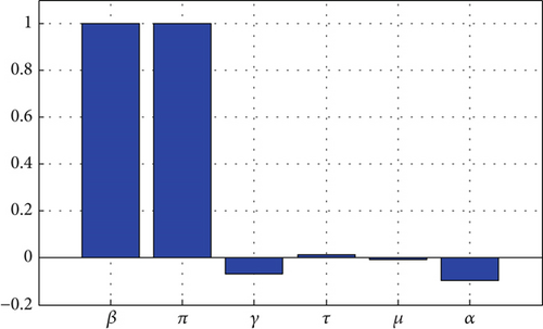
Based on the system parameters, sensitivity indices fall into two categories: positive and negative, as shown in Figure 2. A positive sign of the sensitivity index of to the system parameters has epidemiological implications because it means that changing any parameter in this category will result in an increase or decrease in the value, which in turn causes an increase or decrease in the burden of smokers in the interacting human populations. The community’s expansion of cigarette smoking is likely to be significantly influenced by the parameters with positive indices β, π, and τ if their values increase. Furthermore, the increasing values of the parameters μ, γ, and α, which have negative sensitivity indices, result in a decrease in the prevalence of tobacco usage within the society.

4. Optimal Control Model

This section is aimed at providing optimal intervention strategies for cigarette smoking addiction by illustrating system (1) and formulating an optimal control problem with two control variables u₁(t) and u₂(t). The control u₁(t) shows initiatives aimed at teaching the public about the dangers of cigarette smoking and keeping the vulnerable away from addicts through marketing. Public education about the health risks associated with smoking cigarettes can reduce the likelihood that ex-smokers will relapse and that nonsmokers will convert to smokers, as well as the likelihood that someone will start smoking after coming into contact with a smoker and develop an addiction [18, 19]. In order to provide an adequate treatment for cigarette smoking addicts, the control variable u₂(t) is used. Cigarette smoking can be treated with a variety of methods, such as behavioral counseling and medicines. These interventions not only lessen the intensity of withdrawal symptoms but also improve the likelihood of successful smoking cessation [19]. We get the following optimal control model after incorporating the controls into system (1):

()

The purpose of introducing the control variables is to find the best possible solution at the lowest possible cost to decrease the number of cigarette smoking addicted individuals who are responsible for the spread of cigarette smoking in the population. Thus, the control variables u₁ and u₂ minimizes following is the objective functional subject to the optimal control model (30):

()

where T is the final time, c₁ and c₂ are weight constants of the smoker and addicted population, respectively, while w₁ and w₂ are the weight coefficients associated with each distinct control measures are quadratic [13, 14, 25]. Our goal is to reduce both the quantity of illnesses and expenses. Therefore, we want to achieve an ideal set of restrictions

in which

4.1. Existence of Optimal Controls

We demonstrate in this section that there are such optimal control functions that, for the finite intervention period, minimize the cost function.

Theorem 7. A pair of optimal controls, , exists such that

()

where the closed set is U = {u_i(t): u_i(t) is measurable on [0, t_f], 0 ≤ u_i < 1, i = 1, 2} subject to the beginning circumstances of the control system (29).

Proof 9. We need to validate the following five terms in light of the findings in [20, 24] in order to demonstrate the existence of optimum controls triples.

i.
The set of controls and associated state variables is not empty.
ii.
A closed and convex measurable control set.
iii.
The right side of the state system was bounded by a linearized function in the state and control variables that varied according to time and state variables.
iv.
The cost-functional integrand, g(x, u), is convex on ϑ.
v.
There are constants b₁, b₂ > 0 and b₃>1 such that the integrand of the objective functional satisfies
- i.
  Take note that the dynamics model (29) for cigarette smoking is bounded. It follows that the state system solutions (30) are bounded and continuous for all valid control functions in ϑ. Furthermore, the functions on the right side of the model Equation (30) satisfy the Lipschitz condition with respect to state variables. Consequently, the (Equation 30) solutions of the system are bounded. The set ϑ is therefore not empty.
- ii.
  By definition, ϑ is closed since the control set ϑ = [0, 1]². Additionally, for any two points y, z∈ϑ such that (z = (z₁, z₂) and y = y₁, y₂). According to Pang’s [19] definition of a convex set, λy_i + (1 − λ)z_i ∈ ϑ_i, for every λ ∈ [0, 1]. Hence, ϑ_i implies that λy_i + (1 − λ)z_i ∈ ϑ.
- iii.
  In order to verify this condition, we used the approach adopted by [14]. Let the right hand side of the system (Equation 29) and its solution be represented by h and θ, respectively. It follows that

Hence,

where L₁ = 2(1 − u₁)λ + μ, L₂ = 2α + μ, L₃ = 2γ + 2u₂ + δ + μ, |L₄ = 2η + μ, and M = max{L₁, L₂, L₃, L₄}. Thus, the state system (Equation 30) is clearly uniformly Lipschitz continuous and with this condition (3) is satisfied.

iv.
The integrand g(t, x, u) of the cost functional is given by

Let y = (y₁, y₂) and z = (z₁, z₂) ∈ ϑ and ϖ ∈ [0, 1]. Then, we have

Therefore,

which shows that h(t, u) is a convex function [19]. Since the sum of two convex functions is convex, so that g(t, x, u) is convex function.

v.
Finally, we have

where b₁ = 1/2min{w₁, w₂}, b₂ > 0, and b₃ = 2.

As a result, the objective function can be minimized by an ideal control. The proof is now complete.

4.2. The Hamiltonian and Optimality System

The optimal pair [13] satisfies the necessary conditions, which we obtained by applying Pontryagin’s minimum principle. Inline of this, we were able to derive a Hamiltonian (

) that is defined as follows:

()

Consequently, a reduced Hamiltonian function with regard to

is obtained by substituting the set of Equation (32)

where the adjoint variables are λ_i, for i = 1, ⋯, 4. The adjoint variables can be produced by applying Pontryagin’s minimum principle, according to the following theorem.

Theorem 8. For an optimal control set and that minimizes over U, there is an adjoint variables, λ_i, for i = 1, ⋯, 4 such that

()

with the terminal (transversality) conditions λ_i(t_f) = 0, for i = 1, 2, 3, 4. Furthermore, the optimal controls

are represented by

where

Proof 10. We calculate the derivative of the Hamiltonian function () of Equation (32) with respect to N, S, A, and R, respectively, in order to determine the form of the adjoint equations. Next, the obtained adjoint or co-state equation is provided by

with transversality conditions λ_i(t_f) = 0 for i = 1, 2, 3, 4. To obtain the control value, we compute the partial derivative of Hamiltonian given by

Obviously, after derivation of Hamiltonian () with respect to the controls the result becomes

If you solve for (u₁, u₂) it gives

The following results from the minimality criterion and boundedness on :

where

This completes the proof of the theorem.

5. Numerical Simulations

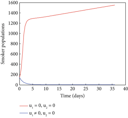
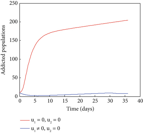
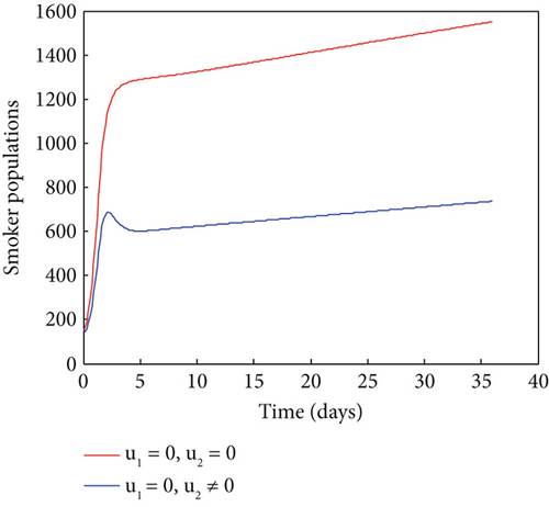
This section presents numerical solutions of system (1) and (30) for various model parameter values. It is demonstrated that the results of these simulations accord with the qualitative behavior of the system solutions. With N(0) = 155, S(0) = 150, A(0) = 10, R(0) = 43, to investigate how the factors affected the dynamics of cigarette smoking addiction, we performed a numerical simulation. We used various parameters with constant variables with varying initial values so that N + S + A + R. The average life expectancy in Ethiopia is 66.71 years; hence the natural death rate is calculated as μ = 1/(66.71 × 12) per day [30]. We provide a numerical example of the optimal control issue solution in system ref1 in this section. We employ the forward–backward sweep approach described in Lenhart and Workman’s book14 for this purpose. Using the parameter values listed in Table 2, Matlab software carried out numerical simulations of the models (1) and (29).

Table 2. Values of parameters used in simulations.

Parameter	Value	Reference
π	1037	Assumed
μ	1/66.71 × 12 per month	[30]
δ	0.45	[23]
γ	0.06	[23]
τ	0.023	[23]
β	0.6234	[31]
α	0.825	Assumed
ρ	0.075	Assumed

For the numerical simulation of the cigarette smoking addiction model, we took into consideration the following three approaches:

1.
Strategy 1: Teaching side effects of smoking cigarettes (u₁ ≠ 0&u₂ = 0),
2.
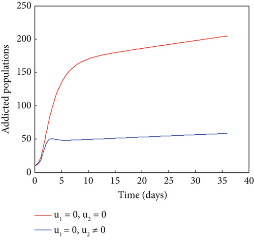
Strategy 2: Taking care of those with addictions (u₁ = 0&u₂ ≠ 0),
3.
Strategy 3: Combinations of two controls (u₁ ≠ 0&u₂ ≠ 0).
1.
Only teaching side effects of smoking cigarettes (u₁ ≠ 0&u₂ = 0)

In this technique, we employed control u₁ to optimize the objective function J in Equation (30), while setting the control u₂ to zero. Figure 3 illustrates how the number of smokers and addicts is considerably lower in situations where control is present than in those where it is not. However, in Figure 3a, the number of smoker individuals eliminated in the first week. This suggests that the prevalence of smoking will decrease if a larger population is aware of the negative effects of smoking cigarettes. In contrast, Figure 3b shows that although the number of addicts appears to have decreased in the first week, the ineffectiveness of the technique causes the addicts to relapse. Therefore, it is an ineffective technique to address the population’s addiction to smoking cigarettes. This implies that the addiction to smoking cigarettes cannot be totally overcome in the given amount of time using this approach.

2.
Taking care of those with addictions only (u₁ = 0&u₂ ≠ 0)

In the second scenario, we simulate the control system without the use of the initial strategy u₁. Figure 4 makes it clear that, when the technique was used instead of having no control, fewer people became smokers and addicts. In this case, the technique used appears to be successful in lessening the burden of addiction during the intervention phase. As such, it might be regarded as the best option for handling the addiction to smoking cigarettes.

3.
Combinations of two controls (u₁ ≠ 0&u₂ ≠ 0)

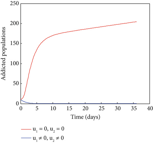
Lastly, we show the results of maximizing the goal function using the combined controls approach. In Figure 5, the related simulation results are displayed. This figure makes it clear that, in comparison to a situation where there is no control, the number of smokers and addicts has significantly decreased as a result of the control method. As a result, the intervention technique works to reduce the number of smokers and addicts within the designated time frame. Thus, in order to prevent addiction, policymakers may decide to employ this integrated strategy.

6. Cost-Effectiveness Analysis

In this subsection, we should design the best optimal and cheapest strategies for minimizing the cigarette smoking dynamics. This strategy was developed using the incremental cost-effectiveness ratio method (ICER). Besides, ICER can be expressed as the values obtained from the difference in averted costs between two strategies to the difference in the total number of infected averted [14]. The infected averted is calculated by the difference between the cigarette smoker using controls and the cigarette smoker if there are no controls, whereas the cost saved is computed by applying the cost functional given as and over time [24]. Therefore, the data we obtained in Table 3 was used to calculate the ICRE and obtain as written the following:

Table 3. Total infected saved and cost avoided for three strategies.

Strategy	Description	Total of infected people	Dollars ($)
1	Prevention individuals	3544.72	1411.30
2	Treatment	3692.54	2248.40
3	Prevention and treatment	5016.44	3256.62

Therefore, the data we obtained in Table 3 used to calculate the ICRE and obtain as written in the following:

Table 4 shows the number of infections averted with ICER for all strategies based on the results in Table 3.

Table 4. Total infected saved and cost incurred as a result of using ICER.

Strategy	Total of infected people	Dollars ($)	ICER
1	3544.72	1411.30	0.398
2	3692.54	2248.40	5.662
3	5016.44	3256.62	0.761

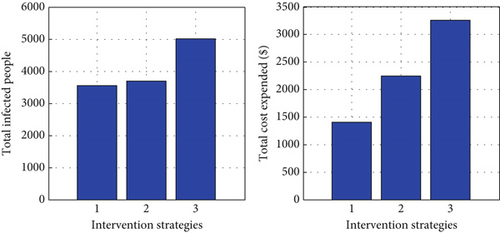
Table 4 compares Interventions 1 and 2. The table shows that ICER (2) is higher than ICER (1). It implies Strategy 2 is expensive and unlikely to save lives. As shown in Figure 6, Strategy 1 saves more people than Strategy 2. Then, we removed 2 from the competing strategies. The ICER of Strategies 1 and 2 is then calculated, as indicated in Table 5.

Table 5. The total number of infections avoided and the cost of employing ICER.

Strategies	Total of infected people	Dollars ($)	ICER
1	3544.72	1411.30	0.398
3	5016.44	3256.62	0.562

Table 5 compares the Interventions 1 and 3. From the table, we have seen that ICER (3) is higher than ICER (1). It implies Strategy 3 is more expensive. Consequently, we suggested that Strategy 3, which involves educating individuals to keep them away from the addicted population, is the optimal and cheapest intervention to minimize the smoking dynamics.

7. Conclusion

In this work, we developed and examined a mathematical model that captures cigarette smoking dynamics with optimal control and cost-effective strategies. Firstly, we show that the model’s solution is positive and bounded with the given initial conditions in a specific, meaningful set. This confirms the model’s well-posedness both mathematically and epidemiologically. Besides, we computed the model’s equilibrium points and demonstrated that they are both locally and globally asymptotically stable using the Jacobian matrix and Lyapunov functions, respectively. Also, we studies of the model’s sensitivity analysis of basic reproduction number have identified a parameter that has the most impact on the dynamics of smoking cigarettes. Furthermore, we extended the smoking dynamics model to the optimal control model involving two controls, such as teaching the public about the dangers of cigarette smoking to keep the susceptible humans away from addicts and treatment for the addicted population. Then, using Pontryagin’s minimum principle, the essential conditions of the optimal control model are examined. Then, we estimate the cost-effectiveness analysis utilizing the incremental ratio approach. Finally, our findings align with those of [19], indicating that educating the public about the risks of cigarette smoking and providing treatment is the most cost-effective approach. If there is a limited resource, our result suggested that a strategy that involves educating individuals to keep them away from the smoking addiction population is the most optimal and least costly intervention to minimize the smoking dynamics. In the future, we will propose considering calibrating the model to available data to estimate the model parameters and applying fractional calculus to the work to account for the memory effect in corruption dynamics. Moreover, the young researchers can expand on this study by including the stochastic model technique, individual age structure, environmental factors, and media roles.

Conflicts of Interest

The authors declare no conflicts of interest.

Author Contributions

Conceptualization, B.Z.A., D.E.T., and T.D.K.; validation, B.Z.A., T.D.K., and M.A.-a.; formal analysis, B.Z.A., D.E.T., T.D.K., and M.A.-a.; investigation, B.Z.A., T.D.K., and M.A.-a.; resources, B.Z.A., D.E.T., and M.A.-a.; data curation, B.Z.A., T.D.K., and M.A.-a.; writing—original draft preparation, B.Z.A., D.E.T., and T.D.K.; writing—review and editing, B.Z.A. and M.A.-a.; visualization, T.D.K. and M.A.-a.; supervision, T.D.K. and M.A.-a. All authors have read and agreed to the published version of the manuscript.

Funding

The authors declare that no financial support was received for the research, authorship, and/or publication of this article.

Open Research

Data Availability Statement

All data supporting the findings of this study are included within the article.

References

1 Darby S. C. and Pike M. C., Lung Cancer and Passive Smoking: Predicted Effects From a Mathematical Model for Cigarette Smoking and Lung Cancer, British Journal of Cancer. (1988) 58, no. 6, 825–831, 3224084.
10.1038/bjc.1988.319
CAS PubMed Web of Science® Google Scholar
2 World Health Organization, WHO Global Report on Trends in Prevalence of Tobacco Use 2000-2030, 2024, World Health Organization.
Google Scholar
3 Summerville E. D., A Mathematical Model for Lung Cancer: The Effects of Second-Hand Smoke and Education, 2000, University of Puerto Rico-Cayey.
Google Scholar
4 Leppan LNBD from Reality, Separating Myth, Tobacco Control and Tobacco Farming, Tech. Rep., 2014.
Google Scholar
5 Murray J. D., Mathematical Biology: I. An Introduction (Interdisciplinary Applied Mathematics), 2007, Springer.
Google Scholar
6 Durkin S., Brennan E., and Wakefield M., Mass Media Campaigns to Promote Smoking Cessation Among Adults: An Integrative Review, Tobacco Control. (2012) 21, no. 2, 127–138, https://doi.org/10.1136/tobaccocontrol-2011-050345, 2-s2.0-84857252761, 22345235.
10.1136/tobaccocontrol-2011-050345
PubMed Web of Science® Google Scholar
7 Gul Z., Qualitative Behavior of Giving up Smoking Models, Bulletin of the Malaysian Mathematical Sciences Society. Second Series. (2011) 34, no. 2, 403–415.
Google Scholar
8 Castillo C., Jordan G., and Rodriguez A., Mathematical Models for the Dynamics of Tobacco Use, Recovery. and Relapse, Technical Report Series, 1997.
Google Scholar
9 Sharomi O. and Gumel A. B., Curtailing Smoking Dynamics: A Mathematical Modeling Approach, Applied Mathematics and Computation. (2008) 195, no. 2, 475–499, https://doi.org/10.1016/j.amc.2007.05.012, 2-s2.0-37349018244.
10.1016/j.amc.2007.05.012
Web of Science® Google Scholar
10 Zaman G., Optimal Campaign in the Smoking Dynamics, Computational and Mathematical Methods in Medicine. (2011) 2011, no. 1, 163834, https://doi.org/10.1155/2011/163834, 2-s2.0-79953290764, 21461044.
10.1155/2011/163834
PubMed Web of Science® Google Scholar
11 Lahrouz A., Omari L., Kiouach D., and Belmaâti A., Deterministic and Stochastic Stability of a Mathematical Model of Smoking, Statistics & Probability Letters. (2011) 81, no. 8, 1276–1284, https://doi.org/10.1016/j.spl.2011.03.029, 2-s2.0-79956207923.
10.1016/j.spl.2011.03.029
Web of Science® Google Scholar
12 Fekede B. and Mebrate B., Sensitivity and Mathematical Model Analysis on Secondhand Smoking Tobacco, Journal of the Egyptian Mathematical Society. (2020) 28, no. 1, https://doi.org/10.1186/s42787-020-00108-1.
10.1186/s42787-020-00108-1
Google Scholar
13 Lenhart S. and Workman J. T., Optimal Control Applied to Biological Models, 2007, Chapman and Hall/CRC.
10.1201/9781420011418
Google Scholar
14 Keno T. D., Dano L. B., and Ganati G. A., Optimal Control and Cost-Effectiveness Strategies of Malaria Transmission With Impact of Climate Variability, Journal of Mathematics. (2022) 2022, no. 1, 5924549, https://doi.org/10.1155/2022/5924549.
10.1155/2022/5924549
Web of Science® Google Scholar
15 Al-arydah M., Mathematical Modeling and Optimal Control for COVID-19 With Population Behavior, Mathematical Methods in the Applied Sciences. (2023) 46, no. 18, 19184–19198, https://doi.org/10.1002/mma.9619.
10.1002/mma.9619
Web of Science® Google Scholar
16 Sun C. and Jia J., Optimal Control of a Delayed Smoking Model With Immigration, Journal of Biological Dynamics. (2019) 13, no. 1, 447–460, https://doi.org/10.1080/17513758.2019.1629031, 2-s2.0-85068232897, 31189458.
10.1080/17513758.2019.1629031
PubMed Web of Science® Google Scholar
17 Eamwa N. I., Optimal Control for Smoking Epidemic Model, Advances in Social Science, Education and Humanities Research. (2020) 528.
Google Scholar
18 Omar Khyar J. D. and Allali K., Mathematical Analysis and Optimal Control of Giving Up the Smoking Model, International Journal of Differential Equations. (2021) 2021, 13, https://doi.org/10.1155/2021/8673020.
10.1155/2021/8673020
Google Scholar
19 Pang L., Liu S., Zhang X., and Tian T., The Cost-Effectiveness Analysis and Optimal Strategy of the Tobacco Control, Computational and Mathematical Methods in Medicine. (2019) 2019, no. 1, 8189270, https://doi.org/10.1155/2019/8189270, 2-s2.0-85062345403.
10.1155/2019/8189270
PubMed Web of Science® Google Scholar
20 Keno T. D. and Legesse F. M., Modelling and Optimal Control Strategies of Corruption Dynamics, Applied Mathematics & Information Sciences. (2023) 17, no. 4, 673–683, https://doi.org/10.18576/amis/170416.
10.18576/amis/170416
Google Scholar
21 Al-arydah M., Assessing Vaccine Efficacy for Infectious Diseases With Variable Immunity Using a Mathematical Model, Scientific Reports. (2024) 14, no. 1, 18572, https://doi.org/10.1038/s41598-024-69651-6, 39127773.
10.1038/s41598-024-69651-6
CAS PubMed Web of Science® Google Scholar
22 Saya R. A. and Khan Z., Mathematical Modeling and Stability Analysis of the Dynamics of Monkeypox Via Fractional-Calculus, Fractals. (2022) 30, no. 10, https://doi.org/10.1142/S0218348X22402666.
10.1142/S0218348X22402666
Google Scholar
23 Van den Driessche P. and Watmough J., Reproduction Numbers and Sub-Threshold Endemic Equilibria for Compartmental Models of Disease Transmission, Mathematical Biosciences. (2002) 180, no. 1-2, 29–48, https://doi.org/10.1016/S0025-5564(02)00108-6, 2-s2.0-0036845274, 12387915.
10.1016/S0025-5564(02)00108-6
CAS PubMed Web of Science® Google Scholar
24 Keno T. D., Makinde O. D., and Obsu L. L., Optimal Control and Cost Effectiveness Analysis of SIRS Malaria Disease Model With Temperature Variability Factor, Journal of Mathematical & Fundamental Sciences. (2021) 53, no. 1, 134–163, https://doi.org/10.5614/j.math.fund.sci.2021.53.1.10.
10.5614/j.math.fund.sci.2021.53.1.10
Google Scholar
25 Aga B. Z., Keno T. D., Terfasa D. E., and Berhe H. W., Pneumonia and COVID-19 Co-Infection Modeling With Optimal Control Analysis, Frontiers in Applied Mathematics and Statistics. (2024) 9, 1286914, https://doi.org/10.3389/fams.2023.1286914.
10.3389/fams.2023.1286914
Web of Science® Google Scholar
26 Salle L. and Joseph P., The Stability of Dynamical Systems, 1976, Society for Industrial and Applied Mathematics, https://doi.org/10.1137/1.9781611970432.
10.1137/1.9781611970432
Google Scholar
27 Chien F. and Shateyi S., Volterra–Lyapunov Stability Analysis of the Solutions of Babesiosis Disease Model, Symmetry. (2021) 13, no. 7, https://doi.org/10.3390/sym13071272.
10.3390/sym13071272
Web of Science® Google Scholar
28 Li J., Yang Y., and Zhou Y., Global Stability of an Epidemic Model With Latent Stage and Vaccination, Nonlinear Analysis: Real World Applications. (2011) 12, no. 4, 2163–2173, https://doi.org/10.1016/j.nonrwa.2010.12.030, 2-s2.0-79955524408.
10.1016/j.nonrwa.2010.12.030
Web of Science® Google Scholar
29 Zahedi M. S. and Kargar N. S., The Volterra–Lyapunov Matrix Theory for Global Stability Analysis of a Model of the HIV/AIDS, International Journal of Biomathematics. (2017) 10, no. 1, 1750002, https://doi.org/10.1142/S1793524517500024, 2-s2.0-84969916166.
10.1142/S1793524517500024
Web of Science® Google Scholar
30 UN-World, https://www.macrotrends.net/countries/ETH/ethiopia/death-rate%27%3EEthiopiaDeathRate1950-2020%3C/a%3E.www.macrotrends.net. Retrieved 2020-06-10.
Google Scholar
31 Adhana M. A. and Mekonnen T. T., A Mathematical Model Analysis of Smoking Tobacco in the Case of Haremaya Town; Ethiopia, International Journal of Research Studies in Science, Engineering and Technology. (2019) 6, no. 2.
Google Scholar

All articles

Optimal Control Analysis of Smoking Dynamics Model With Cost-Effective Strategies

Abstract

1. Introduction

2. Model Formulation

3. Model Analysis

3.1. Invariant Region

3.2. Positivity of the Solutions

3.3. Cigarette Smoking–Free Equilibrium

3.4. The Basic Reproductive Number

3.5. Stability Analysis of Cigarette Smoking–Free Equilibrium

3.6. Endemic Equilibrium and Its Stability Analysis

3.7. Sensitivity Analysis

4. Optimal Control Model

4.1. Existence of Optimal Controls

4.2. The Hamiltonian and Optimality System

5. Numerical Simulations

6. Cost-Effectiveness Analysis

7. Conclusion

Conflicts of Interest

Author Contributions

Funding

Open Research

Data Availability Statement

References

Figures

References

Information

About Wiley Online Library

Help & Support

Opportunities

Connect with Wiley

Optimal Control Analysis of Smoking Dynamics Model With Cost-Effective Strategies

Abstract

1. Introduction

2. Model Formulation

3. Model Analysis

3.1. Invariant Region

3.2. Positivity of the Solutions

3.3. Cigarette Smoking–Free Equilibrium

3.4. The Basic Reproductive Number

3.5. Stability Analysis of Cigarette Smoking–Free Equilibrium

3.6. Endemic Equilibrium and Its Stability Analysis

3.7. Sensitivity Analysis

4. Optimal Control Model

4.1. Existence of Optimal Controls

4.2. The Hamiltonian and Optimality System

5. Numerical Simulations

6. Cost-Effectiveness Analysis

7. Conclusion

Conflicts of Interest

Author Contributions

Funding

Open Research

Data Availability Statement

References

Figures

References

Related

Information