UAV Group Distribution Route Optimization Under Time-Varying Weather Network
Abstract
The rapid advancement in unmanned aerial vehicle (UAV) technology has marked a transformative shift in various industries, with logistics distribution service being one of the prime sectors reaping the benefits. UAVs offer substantial benefits in speed, cost, and reach, promising to revolutionize logistics, especially in remote areas. On the one hand, they are poised to meet demands for quick and versatile delivery options. On the other hand, their deployment comes with challenges. Weather variabilities such as rainfall, wind speed, and the need for safe take-off intervals can compromise UAV safety and operation. Conventional route optimization often overlooks these dynamic factors, resulting in inefficient or unworkable delivery routes. The repeated time-consuming calculations are caused by repeated trials when making UAV group distribution plans. Recognizing these gaps, this study proposes a data representation to effectively transform the flight flyable area of UAVs into a time-varying network that maintains spatiotemporal connectivity and establishes a mathematical model that represents the complexities of UAV group distribution. Then, a multistage dynamic optimization algorithm specifically tailored for large-scale time-varying network distribution route search is designed to obtain the stable and optimal solution. Subsequent experimental validations on actual case datasets have confirmed the correctness, effectiveness, and adaptability of the algorithm. Benchmarking against traditional CPLEX methods demonstrated that the algorithm not only rivals the best solutions but does so with a 38.8 times increase in computational speed. When pitted against the shortest path Dijkstra and A∗ algorithms, the method consistently outperformed, delivering solutions up to 3.5 times faster in large-scale applications. Moreover, the parameter sensitivity analysis is performed on the algorithm by adjusting the safe flight thresholds of rainfall and wind speed parameters and revealed that the performance of the algorithm has a strong positive correlation with the size of the time-varying network.
1. Introduction
The integration of unmanned aerial vehicles (UAVs) into various sectors represents a paradigm shift in operational efficiency, with high-precision trajectory control algorithms [1] serving as the linchpin for this technological revolution. UAVs have transcended their initial military use and are now omnipresent in commercial, humanitarian, and innovative applications, each harnessing the unique capabilities of these versatile aerial platforms. In the humanitarian sphere, UAVs play a pivotal role in disaster relief operations, offering rapid response capabilities to areas rendered inaccessible by catastrophe. High-resolution images from UAV-mounted cameras enable precise damage assessments while payload-carrying UAVs can deliver essential supplies to isolated victims. In the realm of mobile edge computing, UAVs serve as aerial computing nodes [2–4], expanding network coverage and processing data at the edge of the network. This application is particularly beneficial in large-scale events or emergencies where ground infrastructure may be overwhelmed or compromised. In application domains where it is difficult or, to some extent, impossible for humans to monitor the field, such as environmental monitoring, noise level observation, ultraviolet level measurement, or pollution level tracking, the integration of UAVs into wireless sensor networks not only expands the coverage of network applications but also enhances the communication efficiency between the network and control centers [5]. In logistics and transportation, UAVs offer unprecedented solutions to last-mile delivery challenges in the fields of terminal logistics distribution, emergency logistics distribution, and military logistics distribution. They circumvent terrestrial constraints, such as congested roadways and remote locations, thereby enhancing the efficiency and reach of delivery services. The potential of UAVs in this domain is not merely theoretical; major corporations like Amazon and Google are investing heavily in UAV delivery systems, signaling a substantive shift in the logistics industry [6]. The outbreak of COVID-19 in 2020 underscored the utility of UAVs in public health crisis management. UAVs were deployed for contactless delivery and disinfection operations, demonstrating their capacity to adapt to and address emergent societal needs. In China, e-commerce giants such as JD.com and tech-forward delivery platforms like Ele.me have recognized the transformative potential of UAVs, investing in research and piloting UAV-based delivery services [7]. Such initiatives suggest that the UAV distribution mode is not just a fleeting trend but rather a fundamental component of future logistical frameworks. Additionally, it is crucial to consider some ethical implications when UAVs deliver goods in populated areas. Appropriate regulations and guidelines to ensure safety and privacy safeguards will be essential to mitigate potential negative impacts of UAVs on the community. Transparency and communication with the public about the use of UAV technology in their environment can help address concerns and build trust in the responsible and ethical use of UAV delivery systems. UAV route optimization needs a consideration of safety for both the UAV and people living in the populated areas. If a UAV is operating in adverse weather conditions, such as strong winds or heavy rain, there is a risk of the UAV losing control or malfunctioning, which could potentially lead to damage or injury in populated areas. It is important to prioritize the safety of the community when optimizing routes for UAVs, especially in dynamic weather conditions. The potential invasion of privacy when UAVs is operating in populated areas. This could raise concerns about privacy rights and the need for transparency and accountability in the use of UAV technology in populated areas. In summary, while the delivery application of UAVs is primarily a technical issue, the ethical and social impacts must be fully considered during its application to ensure the responsible and sustainable development of the technology.
However, the deployment of UAVs is not without its challenges. Weather variability, including factors like rain, wind, and the necessity for safe intervals between take-offs, poses significant risks to UAV safety and operational reliability. Traditional routing optimization methods tend to ignore these dynamic elements, resulting in suboptimal or impractical delivery pathways. Moreover, the process of devising UAV distribution plans is often slow by time-intensive recalculations due to trial and error. Despite numerous existing UAV distribution methods, a dedicated UAV group distribution strategy is anticipated to emerge as a key approach to revolutionize future transportation and logistics. It aims to facilitate three-dimensional, flexible use of airspace and potentially address the complexities of urban air traffic. Constraints in UAV group path planning typically include turn angles, flight speeds, altitudes, and ascent and descent angles, among others. A significant oversight in the current body of research is the lack of consideration for runway number limitations and their impact on UAV take-off, which necessitates safe intervals between launches to ensure safety. Additionally, there is a gap in the literature regarding the conversion of weather data into actionable flight area information for UAV route planning.
Addressing the identified challenges, this research introduces a novel data representation method that effectively transforms UAV flight areas into a dynamic, time-sensitive network, preserving spatial and temporal connectivity. A comprehensive mathematical model is also proposed that encapsulates the intricacies of managing UAV group distribution. To navigate the complexities of large-scale, time-varying network distribution, a bespoke multistage dynamic optimization algorithm has been developed. This algorithm seeks to deliver stable and optimal routing solutions, considering the limitations posed by weather conditions, safe take-off sequencing, and no-fly zones. By integrating weather data into the UAV route planning process and respecting the self-imposed constraints of the UAV group, this approach stands to redefine the efficiency and safety standards of UAV logistics, setting the stage for a new era in transportation and distribution services.
Therefore, the motivation behind this paper is twofold. First, the goal is to address the dynamic weather conditions that vary with time and space. These conditions significantly impact the safe flyable areas for UAVs, thereby transforming the distribution route optimization into a large-scale and intricate problem. The ever-changing weather patterns demand a flexible and robust approach to route planning to ensure UAVs can navigate safely and efficiently. Second, the logistical constraints imposed by the limited number of available runways and the need to maintain safe take-off intervals for UAVs are taken into account. Such operational limitations further complicate the route optimization process, necessitating a careful balance between runway availability and the timing of UAV deployments. To tackle these challenges and to efficiently solve the complex problem at hand, this paper proposes the development of an effective algorithm designed to generate optimized distribution routes for UAV groups. The goal is to ensure stability and optimality in the calculation results and to increase computational efficiency. This will be achieved by precomputing certain data to avoid redundancy in calculations, thereby reducing the computational load and enabling rapid and repeated planning iterations. Through this approach, the goal is to contribute a novel solution to the problem of UAV group distribution route optimization, taking into account the multifaceted factors that ensure safe and efficient UAV flight operations.
- •
A spatiotemporal expression method is proposed to convert future wind speed and rainfall weather data into a UAV flyable area. Based on this, a time-varying network that meets flight safety restrictions and spatiotemporal connectivity is constructed [8].
- •
A mathematical model of the UAV group distribution route was established, taking into account the constraints of the safe flight and take-off time interval of the UAV group under the time-varying network.
- •
A multistage dynamic optimization algorithm is designed, which is suitable for solving the large-scale UAV group distribution route problem. This provides a feasible solution or idea for solving similar problems like this.
- •
The proposed algorithm was experimentally tested for correctness, effectiveness, and parameter sensitivity based on actual case data, proving that it can effectively reduce calculation time and maintain the stability of calculation results.
In the subsequent sections of this paper, Section 2 provides a comprehensive description of the related work in the field relevant to this topic. Section 3 will introduce the specific problem that is being addressed and describe the mathematical model with the assumptions, variables, and equations involved. In Section 4, the methodology for constructing a space–time network that represents all possible movements will be described, and the specific content of the proposed method will be introduced in detail. Section 5 will present the data used to test the model and carry out some experiments to prove the validity of the proposed method. Section 6 will summarize the main findings of this research and highlight the contributions and significance of the work. It will also discuss potential implications, future work, and any limitations of the current study.
2. Related Work
There have been some studies related to UAV distribution, and a literature survey and discussion will be conducted from four aspects: (1) UAV distribution mode, (2) UAV group path planning, (3) weather conditions, and (4) solution methods. The corresponding research results are as follows.
2.1. UAV Distribution Modes
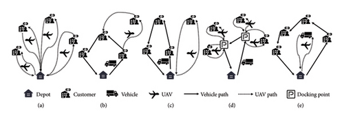
The research in this area can be divided into UAV group distribution, vehicle and UAV collaborative distribution, vehicle and UAV parallel distribution, vehicle-supported UAV distribution, UAV-supported vehicle distribution, and mixed-mode distribution [9]. A schematic diagram of the first five UAV distribution modes is shown in Figure 1. The UAV group distribution only uses UAV to deliver goods as shown in Figure 1(a). The vehicle and UAV cooperative distribution is a common mode in research on vehicle and UAV combined distribution. The vehicle will be equipped with one or more UAVs, which store goods and provide charging services for UAVs during the distribution process as shown in Figure 1(b). And they deliver goods to their respective customer nodes under cooperation [10]. The parallel distribution of vehicles and UAVs mode denotes that the distribution of vehicles and UAVs is independent [11] as shown in Figure 1(c). The UAVs travel to and from the distribution center alone and are only allowed to pick up goods and charge at the distribution center [12, 13]. In the distribution mode of the vehicle-supported UAV, as shown in Figure 1(d), the vehicle serves as an auxiliary to provide goods storage and charging services for helping the UAV perform distribution tasks [13–15]. UAVs shuttle between vehicles and customer points for distributing goods to customers. At the same time, the vehicle drives to the next docking point or stops at the same spot, expecting the UAV to fly back after delivery. In the vehicle distribution mode supported by UAV as shown in Figure 1(e), UAV replenishes the vehicle as an auxiliary to assist the vehicles in performing the distribution tasks [16]. The hybrid model refers to utilizing two or more distribution modes to provide distribution services for customer nodes [17, 18]. As UAVs are continuously used in actual scenarios, the load-bearing capacity and endurance of UAVs will be greatly improved. So although there are many UAV distribution modes at present, pure UAV group distribution will become a large-scale mode to reshape future transportation and logistics, promote the 3D flexible use of airspace, and become a potential game changer in solving urban air traffic challenges [19].
2.2. UAV Group Path Planning
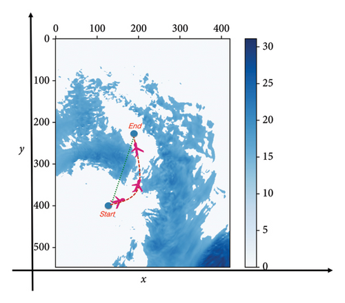
The goal of UAV group path planning is to find a sequence of waypoints connecting the starting point and the destination for each UAV as shown in Figure 2. Generally, the process of generating UAV paths is generated first through proactive planning [20] and then generated through reactive planning during execution [21–23]. Proactive planning focuses on resource scheduling and efficiency, while reactive planning focuses on task execution and safety. The UAV paths generated in proactive planning ensure that the objectives of the planned mission are achieved under predetermined changes in environmental parameters [8]. Reactive planning needs to consider that the route generated during the actual mission execution needs to be adjusted according to real-time changes in the environment. The research content of this article focuses on proactive planning. The common approach taken by most research on proactive planning starts around building a mathematical model of UAV group path planning. In the process of building the model, the environmental constraints, self-constraints, and intracluster constraints of the UAV group are taken into account [24, 25]. The construction methods of its environmental space mainly include the cell method, the landmark method, and the potential field method [26]. The path planning of this problem usually needs to construct the corresponding objective function according to different task requirements or decision-maker preferences [27]. The self-constraints of UAV group path planning are generally turning angle constraints, flight speed constraints, flight altitude constraints, climb angle constraints, dive angle constraints, and so on. Gao [28] presents a multiobjective optimization model for cooperative mission assignment of heterogeneous UAVs that balances mission gains against the risk of UAV losses. Surprisingly, it is noted that existing literature does not consider the impact of runway number limitations on UAV take-off in UAV delivery. This leads to safety considerations for UAVs during take-off, requiring a safe take-off time interval between UAVs.
2.3. Weather Conditions
Weather is a key feature to consider when flying a UAV, as it can affect the speed, distance, and safety of the UAV. In addition, the safety and efficiency of UAV logistics distribution are closely related to the weather conditions. Among them, strong wind, heavy precipitation, and ice accumulation have the most significant impact on flight safety. In bad weather, the probability of damage to UAVs during work increases sharply, bringing significant economic losses to enterprises. DHL, a German freight company, considered using a UAV to deliver a package weighing up to 2 kg. Still, finally, they reluctantly postponed the plan because of weather factors like sudden temperature drops and heavy snow. Therefore, it is of great theoretical and practical significance to schedule the logistics distribution route of UAVs according to the meteorological prediction data. Some literature studies how to accurately predict weather factors that affect UAV flight, such as wind speed and solar radiation [29, 30]. And some literature studies atmospheric temperature and how to affect the energy consumption of UAV batteries [31–33]. Stevens [34] studied how UAV operations may be affected by weather. Peng and Murray [11] considered the impacts from winds and rainfalls that change drones’ preferable/available travel time. Some studies on UAV path planning assume that wind can be static and consistent [35, 36], while others assume that wind can be dynamic and known in advance [31, 33, 37, 38]. Cheng et al. proposed a two-period UAV scheduling model considering stochastic weather, and their use of robust optimization for decision-making can mitigate the risk of delivery delays due to weather uncertainty [39]. In real-life scenarios, UAVs are prohibited from passing through the flight area during this period due to bad weather such as rainfall exceeding the safety threshold as shown in Figure 2. Therefore, when planning the route of the UAV, it is important to avoid passing through these no-fly areas. However, in the existing literature, no literature has not been found that consider converting weather data into flyable area data for UAVs for route planning.
2.4. Solution Methods
Due to the NP-hard nature of the UAV group path planning problem, the solution methods used in the existing literature include MLP [40, 41], declarative modeling [20, 31, 42, 43], computer simulation [44, 45], machine learning [46], and heuristic algorithms [47]. Although there are so many solution methods, the mainstream algorithms used in most literature are mainly divided into classical algorithms [48, 49] and metaheuristic algorithms. Classic algorithms include search-based algorithms such as Dijkstra algorithm [50], A∗ algorithm [51], and graph search method. Moro [52] has presented a modification of the A∗ path planning algorithm for a fixed-wing UAV to significantly reduce energy consumption in wireless sensor networks by up to 20% for the UAV and 25% for the network through efficient data collection. These algorithms show good performance in single UAV path planning problems but are difficult to apply to large-scale, high-dimensional, multi-UAV path planning problems. On this basis, some scholars have done more in-depth research and use evolutionary algorithms to solve the problem [47]. Perez-Carabaza et al. [53] studied the improved ant colony algorithm to solve the shortest time problem and stagnation problem of UAV flight trajectory. Rivera et al. [54] studied a superheuristic permutation multiobjective evolutionary algorithm based on ant colonies, integrating preferences into multiobjectives to solve the model. Ni et al. [55] integrated the ant colony algorithm with the neural network algorithm to improve the efficiency of solving three-dimensional paths. These algorithms have high search efficiency and can obtain the optimal solution in a static small global environment [56]. However, as map information increases, search nodes increase significantly, and the route planning problem becomes a large-scale and complex problem, which will make the algorithm calculation time longer [57]. Wang et al. [58] dispatched trajectory planning on flight decks by using hybrid A∗ for initial path generation. Wang et al. [59] combined an artificially guided hybrid A∗ algorithm for initial coarse path searching with an optimization approach for fine-tuning for docking trajectory planning of unmanned surface vehicles. When solving these large-scale problems, the performance and results of evolutionary algorithms are often unstable and cannot give a stable result within a limited time. In addition, there are also some cutting-edge studies using reinforcement learning to solve these problems [60, 61]. Wang et al. [62] offered a comprehensive review of deep reinforcement learning for UAVs to win dogfights. However, reinforcement learning usually requires that the state space should not be too large, but the UAV path delivery problem itself is a problem with a very large state space. Every UAV route, whether it is feasible or not, is a state. So when the search space of paths is slightly larger, the number of paths will fall into a combinatorial explosion. At the same time, the output results of reinforcement learning cannot be guaranteed to satisfy all strong constraints. This requires a repair module to ensure that the results are feasible, but the stability and optimality of the results cannot be guaranteed. Through the above description, each type of solution method has its advantages and disadvantages, and it is difficult to achieve both short calculation time and stable calculation results. Path planning requires constantly querying nodes in the time–space data, inserting and deleting them, and finally forming a route. Therefore, most classical algorithms and metaheuristic algorithms have one thing in common, which is that they require a large amount of calculations to find the shortest path between two points. The work of finding the shortest path between two points can be calculated in advance during the first calculation so that subsequent calculations can reuse the previous work and avoid the time-consuming caused by repeated calculations. In the existing research, no scholars have been found who have proposed a method that combines the data preprocessing process of finding the shortest path between two points in advance with the classic algorithm. This approach would not only prevent redundant computations in subsequent calculations, thereby reducing total processing time, but it would also guarantee stability and optimality in the computational outcomes.
For the state-of-the-art most relevant to the research content of this article, please refer to [11]. In [11], the authors conduct a quantitative analysis of the impact of wind and rain on UAVs, studying a scenario of parallel delivery involving one truck and multiple UAVs. By converting these weather impacts into time-dependent UAV flight times and feasible flyable time windows, they provide a new perspective on how weather conditions affect the truck–UAV distribution system. Their research is concentrated on short-distance deliveries, assuming uniform weather data across the entire service area over a given period, without taking into account the potential variations in weather conditions in localized regions. In their model, each UAV or truck is capable of serving multiple customers within a single mission. The optimization focuses on the allocation of customers to the truck or UAVs and the sequence in which these customers are served. This paper explores the scenario of weather-aware long-distance deliveries conducted by a group of UAVs. The weather data for localized areas within the entire service region change over time, with each UAV designated to serve only one customer. But the optimization efforts in this study are directed toward fine-tuning the safe take-off time intervals for the UAV group and devising flight routes that adhere to weather safety constraints.
3. Problem Formulation
3.1. Problem Description
The problem studied in this article comes from a large logistics company exploring UAV applications. The company hopes to operate a fleet of UAVs for long-distance transport. The problem description is shown in Figure 3. The UAVs take off one after another from a fixed runway every morning and then fly to multiple destinations. Complex and changeable meteorological conditions will endanger the transportation safety of UAV. Therefore, they need to be able to plan the flight route of the UAV based on high-precision weather forecasts to avoid dangerous weather areas and reach the destination within the specified time limit. For the sake of facilitating description and modeling, this article divides the UAV flight area into small regional blocks based on the minimum area covered by the weather forecast. The symbols and notations used in the mathematical formulation are shown in Table 1.

| Sets | Explanations |
|---|---|
| P | Set of all UAVs |
| N | Set of all nodes |
| A | Set of all arcs |
| Parameters | Explanations |
| U | Flight time of the UAV at each node |
| Wind speed value of the UAV p at the node i | |
| Rainfall value of the UAV p at the node i | |
| W | Maximum wind speed |
| R | Maximum rainfall |
| Flight time with traversing arc (i, j) of the UAV p | |
| Wpenalty | Penalty value for not finishing the distribution task |
| H | Interval time of the take-off time between any two UAVs |
| Decision variables | Explanations |
| 1 if the arc (i, j) is traversed by UAV p, and 0 otherwise. | |
| yp ∈ {0, 1} | 1 if UAV p fails to complete the distribution task and 0 otherwise. |
| Time of the UAV p within node i | |
The flight time U of the UAV in each regional block is the same. Each regional block at each period U corresponds with a specific node. With n nodes, there is a directed graph G = (N, A) that arc (i, j) ∈ A and N represents the node-set. And 1 denotes the starting node and n denotes the end node. The weather conditions at time node of each UAV p (p ∈ P) will vary with the time. At the node i, let represent the wind speed value and represent the rainfall value of the UAV p. Only when is less than or equal to the maximum wind speed W and is less than or equal to the maximum rainfall R, the UAV p be allowed to fly safely at the node i. As notations, represents the time required for the UAV to fly from node i to node j, H represents the interval time of the take-off time between any two UAVs, and Wpenalty denotes the penalty value for not finishing the distribution task. When yp is 1, the UAV fails to complete the distribution task. Otherwise, it is 0. The objective is to find a way to minimize the total distribution cost of the system by planning distribution routes for the UAV group, which include the take-off time of each UAV, the order of visiting nodes, and the time of arriving at each node in the graph.
3.2. Model Establishment
The objective function (1) aims to minimize the distribution time of the UAV. Constraint (2) indicates whether the UAV completes the distribution task. Constraints (3) and (4) represent the constraint on the arc balance in the fundamental shortest path problem. Constraint (5) indicates the take-off time constraint among UAVs. Constraints (6) and (7) show that for the UAV p, if the rainfalls and are heavier than R, then , which means no UAV passes through node i and node j. Similarly, constraints (8) and (9) illustrate that for the UAV p, if the rainfalls and are heavier than R, then , which means no UAV passes through node i and node j. Constraints (10) and (11) indicate that if , the time for the UAV to reach a point j is greater than or equal to the time it departs from the node i plus the time consumed on the way from the node i to the node j. If , this constraint is relaxed. Finally, constraint (12) denotes a nonnegative constraint, and constraints (13) and (14) give 0-1 variable constraint. In this model, the value of M is set to 1000 times the value of U, M = 1000U.
4. Solution Approaches
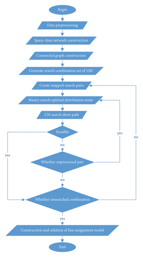
The distribution route planning of UAVs needs to meet the safety requirements of aerial flight and find the shortest and most efficient route set. The safety requirements here include restrictions on the UAV take-off time interval and avoiding the impact of bad weather on the flight. The critical weather factors affecting UAV distribution include wind speed and rainfall, and these factors change in different spatial areas with time. Therefore, when planning the UAV distribution route, this paper first reasonably describes the environmental space of UAV distribution and forms a space–time network that changes with time. Then, a connected network diagram is constructed according to the spatial relationship and time continuity. The connectivity graph data of the space–time network is too large to directly use the mathematical programming solver to solve the mathematical model. So finally, a multistage dynamic optimization algorithm is designed suitable for solving this problem. The algorithm consists of three stages. In Stage 1, the CH (contraction hierarchies) algorithm [63] is devoted to speeding up the calculation of the shortest path. In Stage 2, the binary search algorithm is proposed to accelerate the search for the feasible optimal route in a large number of distribution route choices. In Stage 3, the optimal route assignment model is derived from the UAV feasible route set, has a constraint of the take-off time interval between UAVs, and can be easily solved by the mathematical programming solver. The overall implementation process of the multistage dynamic optimization algorithm is shown in Figure 4.
-
Step 1: Preprocess the weather data at first, using the grid approach to spatially represent the UAV distribution region and divide it into equal-sized unit areas. The duration of the UAV path in each unit area is the same, and the flying state of the unit area at different times will be expressed as distinct space–time nodes.
-
Step 2: After the construction of the space–time network, the unit areas satisfying the relationship of upside-down, left-right, and time continuity between spaces are connected via edges to form the connected graph data.
-
Step 3: Taking into account the influencing elements such as the earliest take-off time and the latest end time of UAV, the search combination set of the UAV route is computed for the subsequent search of the UAV distribution route.
-
Step 4: A candidate combination consisting of a fixed start space–time node and a collection of end space–time nodes is selected from the UAV distribution route search combination set. That fixed starting nodes and various ending nodes will combine to create numerous mapped search pairs.
-
Step 5: The binary search method is employed to rapidly locate the ideal search pair among these mapped search pairs.
-
Step 6: Judging whether there is a node pair for binary search. If no, return to Step 4. Use the shortest path CH algorithm to expedite calculating the shortest path for the selected node pair.
-
Step 7: If the preceding CH algorithm is not feasible, return to Step 6 and resume the CH algorithm by calculating the following new node pair. Otherwise, add it to the set of feasible routes of all UAVs and immediately terminate the current binary search.
-
Step 8: Judging whether there is no combination for UAV route searching. If so, return to Step 4 and start the next binary search.
-
Step 9: According to the feasible route set of UAVs, considering the safe take-off time interval between UAVs, a route assignment model was constructed and the optimal route combination of UAVs.
4.1. Space–Time Network Representation
Unlike the on-road distribution, the distribution space of a UAV is not a road network connected by roads but a relatively open and free-flight space. For generating distribution lines, it is necessary to grid and digitize them first. The grid method used is a method of spatial modeling. It divides the delimited topographic map into units, employs grids of equal size to divide the space, and uses a grid array to represent the whole space.
The shortest path is obtained by searching the free space on this grid network. If the spatial size of one unit defined by the grid is smaller, the environmental information shown by the grid map will be pretty elaborated. However, it has a problem that more knowledge needs to be stored, which will increase the storage overhead and reduce the speed of path planning. In other words, the performance of real-time line planning is not guaranteed. On the contrary, if the spatial size of one unit is larger, the path planning speed will improve because less information is waiting for storage. However, the division of environmental data will encounter the onset of fuzzier, which is not conducive to planning effective paths. Therefore, there is a contradiction between solution speed and space–time cost for the path planning algorithm’s performance, so the unit area size selection is an essential factor. The unit area size selected in this paper follows the experimental data rules. The distribution area is divided into regional blocks according to the minimum range covered by the weather forecast. Each unit area’s length, width, and size are the same, and the flight time U of the UAV in each unit area is provided as the same. In the period U, the flying state of the unit area is determined by the wind speed and rainfall in this period. In other words, it can fly within the unit area in the T period when the wind speed and rainfall are less than the safety threshold, otherwise cannot. (x, y, t) is used to uniquely sign each unit area in a different time, which x represents the coordinate value in the x-axis direction, y represents the coordinate value in the y-axis direction, and t represents one period U. Different colors indicate another feasible state of the unit area, such as dark color denoting the infeasible area while light represents the free-flying space. The whole weather data example of one period is shown in Figure 5.
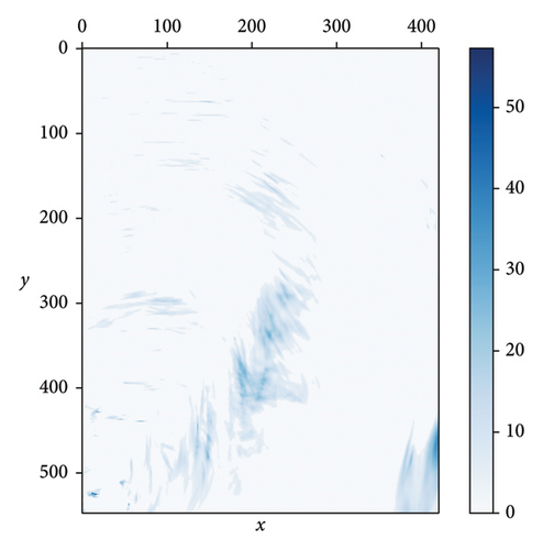
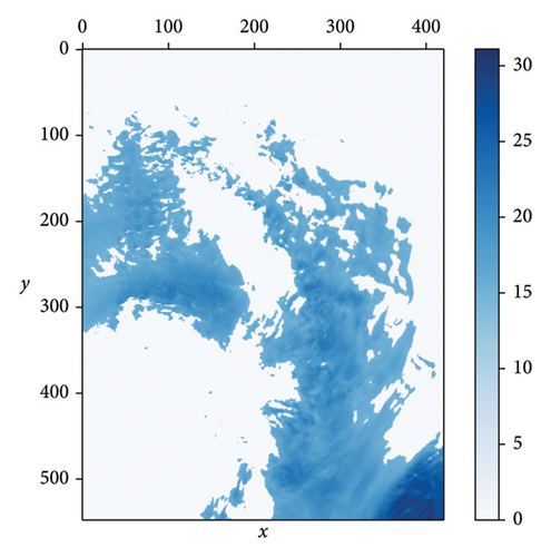
Illustration of Figure 5: The figure on the left and right illustrates the rainfall distribution and wind speed distribution in a single period in the coverage area. Colored areas represent that the rainfall and wind speed exceed the UAV flying safety threshold, while colorless areas indicate that they meet the threshold. In addition, if darker the color, the greater the rainfall and wind speed.
4.2. Connected Graph Construction
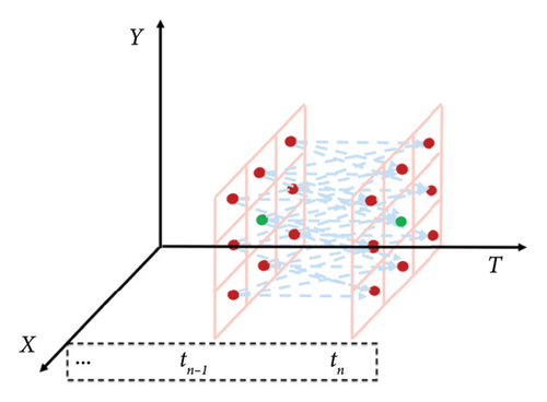
When constructing a connected network, the vertex is each unit area, and an edge is a line in which one unit area connects to the nearby unit area. Because of the up–down and left–right relationship between spaces, it is limited that each unit area can only be directly associated with its upper, lower, left, and right unit areas. Owning to the limitation of the time-continuous relationship, the unit area in the T period can only be connected with that in the following T period. Based on the above two connection limitations, the whole connected network is achieved by construction. The process of edge formation of a connected graph is shown in Figure 6.
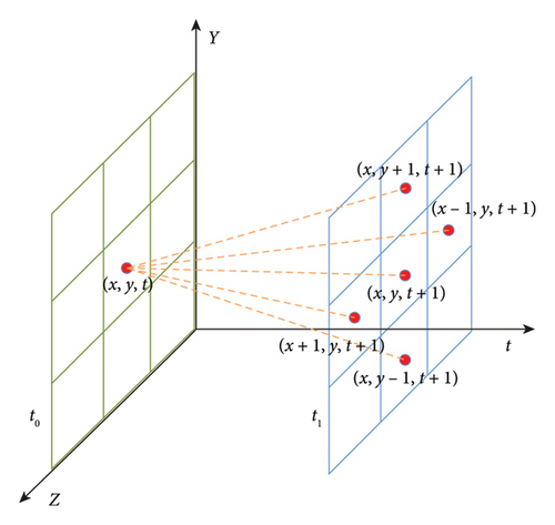
Illustration for Figure 6: If the current cell area is (x, y, t), the cell area connected to the edge forming the connected graph is (x, y, t + 1), (x, y + 1, t + 1), (x, y − 1, t + 1), (x − 1, y, t + 1), and (x + 1, y, t + 1).
Considering that reducing the scale of the connected graph can speed up the algorithm’s search, some optimization methods for designing around the characteristics of the problem need to be proposed to reduce the edge construction of the connected graph. When the starting position O(xo, yo) and the ending position D(xd, yd) are determined, the theoretical minimum flight time ttheory from the start node to the end node is also determined, ttheory = |xo − xd| + |yo − yd|. Based on the theoretical minimum flight time ttheory, the connected graph can be clipped to delete some space–time nodes in advance.
In Figure 7(a), the blue point is the start space–time node O(xo, yo, to), and the space–time nodes around O(xo, yo, to) extend to other nodes to form some edges, and these edges will be some part of the connected graph. Because these edges do not meet the starting position restrictions, becoming a part of the UAV flight path is impossible so that excess edges can be removed. After cropping, the changed graph is shown in Figure 7(b).
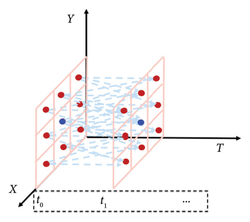
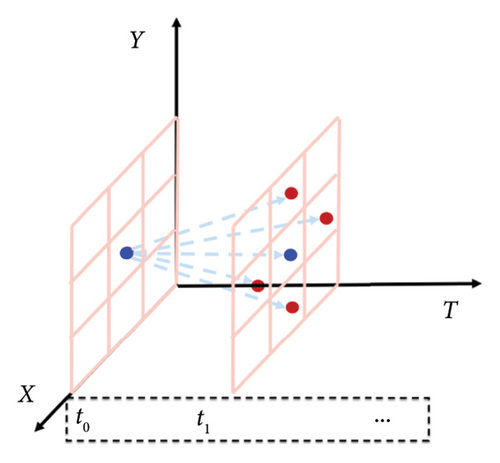
In Figure 8(a), the green point is the end space–time node D(xd, yd, td), and the space–time nodes around D(xd, yd, td) extend to other nodes to form some edges, and these edges will be some part of the connected graph. Tmin is the earliest departure time. When the expression tn − |x1 − x2| − |y1 − y2| − Tmin < 0 is satisfied, these edges can be removed. After cropping, the changed graph is shown in Figure 8(b).
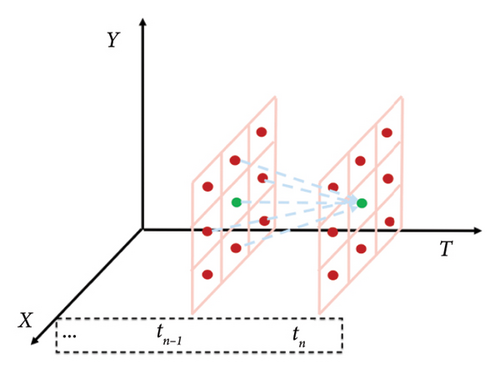
For the intermediate space–time node M(xm, ym, ti) to form some edges, some optimization methods are proposed to remove some invalid edges. Tmax is the latest arrival time. When the expressions ti − |xm − xo| − |ym − yo| < Tmin or ti + |xm − xd| + |ym − yd| > Tmax is satisfied, these edges can be removed.
The density of a graph reflects the proportion of the actual number of edges to the total potential edges that could exist between all node pairs. For directed graphs, this maximum is N × (N − 1), with N representing the node count. Sparse graphs have significantly fewer edges than the maximum, typically on the order of O(N) or linear concerning the number of vertices. In contrast, dense graphs have an edge count nearing the maximum, generally on the order of O(N2). Graph density crucially affects the efficacy of shortest path algorithms, as it influences computational efficiency. Sparse graphs often yield faster computations due to their limited edge count, whereas dense graphs necessitate algorithms capable of efficiently managing a higher volume of edges without overly increasing computation time. Algorithms that minimize unnecessary edge evaluations perform better in sparse graphs, while those that can handle a higher edge volume are preferred for dense graphs. As detailed previously, this paper deals with a connected graph whose nodes are of a known quantity, with no more than 5 incoming or outgoing edges per node, contingent on meeting minimum safety criteria for rain and wind. By adjusting these safety thresholds, control over the graph’s density is exerted. Setting low safety thresholds results in a sparser graph, potentially leading to a scenario where nodes remain unconnected. In contrast, higher thresholds increase the graph’s density, potentially approaching the scenario where nearly every node is connected by 5 incoming and outgoing edges, with the edge count nearing 5N. Thus, the connected graph in this study is inherently sparse by design, and algorithms suited to such a structure are employed, including classical ones like Dijkstra’s algorithm and heuristic-based approaches like the A∗ algorithm.
4.3. Route Search Combination Generation
Based on the space–time network connectivity graph corresponding to the UAV distribution area, different start and end space–time nodes will lead to excessive combinations of UAV distribution routes. A lot of route search combinations will slow down the total calculation time. So a route search combination generation is proposed to form the UAV route search combinations and filter out some infeasible combinations in advance. The specific implementation logic is shown below.
Without considering the weather factors, the shortest flying time of a UAV from the starting unit area O(x1, y1, t1) to the destination unit area D(x2, y2, t2) is |x1 − x2| + |y1 − y2|. So the range of t1 is [Tmin, Tmax − |x1 − x2| − |y1 − y2|], and the corresponding range of t2 is [t1 + |x1 − x2| + |y1 − y2|, Tmax]. Then, by traversing every value in the range t1 when the UAV takes off and combining it with the range t2, all the route search combinations satisfying the time limit can be enumerated.
After the UAV take-off time t1 is determined as , the corresponding route search combination can be selected and numerous mapped search pairs with clear start and end space–time nodes can be created, , representing the fixed flight time of the UAV in one unit area.
4.4. Binary Search Algorithm
If the shortest travel time of a UAV from the starting unit O(x1, y1, t1) to the destination unit area D(x2, y2, t2) is t∗, there must be a feasible route with a travel time longer than t∗. So in this paper, the binary search method is adopted to speed up the search for the mapped search pairs E and find the shortest feasible UAV distribution time and viable route. The Algorithm 1 of the binary search is as follows:
-
Algorithm 1: Binary search algorithm.
-
Require: the initial search combination E
-
Ensure:
- 1.
low = 0, middle = 0, high = Size(E) − 1
- 2.
- 3.
call the CH algorithm to calculate the path r of
- 4.
ifris NULL then
- 5.
Return NULL
- 6.
end if
- 7.
- 8.
call the CH algorithm to calculate the path r of
- 9.
ifris NULL then
- 10.
Return NULL
- 11.
else
- 12.
r∗⟵r
- 13.
end if
- 14.
whilelow ≤ highdo
- 15.
middle = (low + high)/2
- 16.
ifmiddle = 0then
- 17.
low = middle + 1
- 18.
else ifmiddle = Size(E) − 1then
- 19.
low = middle − 1
- 20.
else
- 21.
- 22.
call CH algorithm to calculate feasible path r
- 23.
ifris NULL then
- 24.
r∗⟵r
- 25.
high = middle − 1
- 26.
else
- 27.
low = middle + 1
- 28.
end if
- 29.
end if
- 30.
end while
- 31.
Return r∗
4.5. CH Algorithm
When calculating the shortest path of a large-scale network graph, the Dijkstra algorithm is the most used path planning algorithm between two points. To further provide computational efficiency, the bidirectional Dijkstra algorithm is derived. However, the query efficiency of the algorithm is affected by the structural characteristics of the network graph and the distance between query nodes, which will occasionally reach second-level response but is considerably challenging to achieve the stable output of microsecond-level response. Then, the shortest path CH algorithm is an acceleration technology for finding the shortest path in the network graph that was first proposed by Weisberger et al. [63, 64]. By making full use of the characteristics of the network graph, it preprocesses the original graph first. It calculates the shortest path distance between some points in advance for the convenience of simplifying the number of edges of the network graph and supporting a fast query of the shortest path between two points.
CH algorithm includes path network graph preprocessing and shortest path query. Thanks to the network diagram structure of weather data being rarely updated, some calculations can be performed in advance and then queried. So the query time leaps to the millisecond level. This acceleration is realized by “shortcuts.” It connects the two nonadjacent vertices u to v, and its edge weight is the sum of weights on the shortest path from u to v. Finally, in the shortest path query, these “shortcuts” created in the preprocessing stage are used to improve the search efficiency by skipping the “unimportant” vertices.
4.5.1. Graph Preprocessing
The preprocessing of the CH algorithm generates a multilayer graph structure in that each graph node is in a separate layer. To achieve it, the CH algorithm selects nodes from low to high according to the priority of nodes to perform iterative vertex shrinkage. Each time “shrinking” a node, it will generate corresponding “shortcuts” and form an updated graph structure. To push the shrink operation, the shortest path between the shrink node and others needs to be calculated, “shortcuts” inserted for it, and then, the shrink node marked as processed. Shrinking does not delete the node, but the shrink nodes can be ignored in the rest of the shrinking process.
CH algorithm has proved that sorting the graph nodes in any order and then successively adding shortcuts can ensure the accuracy of the result. However, different sorting methods will have an impact on the efficiency of preprocessing and subsequent search queries. So the priority ordering of nodes should be designed according to the characteristics of the problem. The node shrinkage sorting method uses the priority queue, and the smallest element of the queue has the most shrinkage potential. Considering the characteristics of this problem, only when the wind speed and rainfall of a unit area do not meet the flight conditions, the connectivity of adjacent nodes will be affected, as shown in Figure 9(a). The cell regions C2 and B3 that do not meet flight conditions will form isolated nodes and lead to unbalanced access to neighboring nodes. Some particular points, such as A1, B1, C1, A4, B4, and C4, are unilateral in or out nodes of the whole space–time network. The unilateral in or out node only stores the edge of the outgoing or incoming edge. These above-mentioned nodes all affect the network connectivity, so the affected adjacent nodes should be compressed first and shortcuts to improve the network connectivity. A corresponding new node shrinkage priority weight is designed.

In the above formula, nnode_degree_in is the number of edges that enter the shrink node and nnode_degree_out is the number of edges that go out from the shrink node. By the priority weight values wpriority, the nodes in Figure 9 are compressed in the order shown in Figure 10.

Finally, after the graph preprocessing, some shortcuts are added to the original graph. The new graph is shown in Figure 9(b).
4.5.2. Shortest Path Query
The query phase of the CH algorithm adopts the bidirectional Dijkstra algorithm. In the search process, you can only search from the low-order nodes to the high-order nodes. When querying the shortest path phase, the two-way search conducts from the starting node and the target node and then extends through the “shortcuts” created in the preprocessing stage. One begins the forward search from the starting node, and the other launches the reverse search from the ending node. After the two searches collide in the same node, the shortest path is found, and the two-way search is terminated. Although the overall search process is like Dijkstra’s algorithm, it differs because the search is only for nodes whose shrinkage order is higher than the current node, meaning the search is only for upward-sloping edges. The pseudocode of the bidirectional Dijkstra Algorithm 2 for CH is as follows:
-
Algorithm 2: Bidirectional Dijkstra algorithm.
-
Require: the start node s and end node t
-
Ensure:
- 1.
priority queues: Qf, Qb; sets: Sf, Sb; distance variable: cost
- 2.
initialize: Qf = ∅, Qb = ∅, Sf = ∅, Sb = ∅, cost = MAX
- 3.
Qf⟵(s, df[s]), Qb⟵(t, df[t]), Sf⟵s, Sb⟵t
- 4.
whileQf ≠ ∅ and Qf ≠ ∅do.
- 5.
u⟵poll(Qf), v⟵poll(Qb)
- 6.
Sf⟵u, Sb⟵v
- 7.
forxinadj(u)
- 8.
ifxnot inSf and order[x] > order[u] and df[x] > df[u] + weight(u, x)then
- 9.
df[x] = df[u] + weight(u, x)
- 10.
Qf⟵(x, df[x]), Sf⟵x
- 11.
end if
- 12.
end for
- 13.
ifuinSb and df[u] + db[u] < costthen
- 14.
cost = df[u] + db[u]
- 15.
end if
- 16.
forxinadj(v)
- 17.
ifxnot inSb and order[x] > order[v] and db[x] > weight(x, v) + db[v]then
- 18.
db[x] = weight(x, v) + db[v]
- 19.
Qb⟵(x, db[x]), Sb⟵x
- 20.
end if
- 21.
end for
- 22.
ifvinSf and df[v] + db[v] < costthen
- 23.
cost = df[v] + db[v]
- 24.
end if
- 25.
end while
- 26.
Return cost
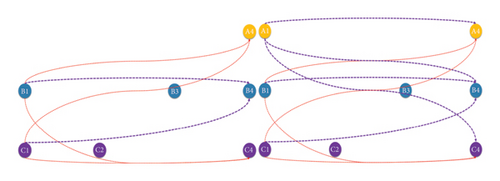
The schematic diagram of the CH algorithm searching the shortest path is shown in Figure 11.
4.5.2.1. Search From C1 to B4
If calculating the shortest path from C1 to B4, it is important to get the upward graph from C1 and the upward graph from B4 at first. Because C1 is the latest shrinking node, there is no upward graph. The upward graph of B4 is shown on the left of Figure 11. In the first iteration, the forward search result is empty, and the reverse search result is B1- > B4 and C1- > B4. Finally, they meet at point C1 and the shortest path is found.
4.5.2.2. Search From A1 to B4
Similarly, the upward graph from A1 and the upward graph from B4 at first will be obtained. The final upward graph of A1 and B4 is shown on the right of Figure 11. In the first iteration, the forward search result is A1- > C4, A1- > B4, and A1- > A4, and the reverse search result is B1- > B4 and C1- > B4. Finally, they meet at point B4 and the shortest path is got.
When selecting an algorithm for finding the shortest path in a graph, it is crucial to consider the characteristics of the graph and the application requirements. CH shines in scenarios where a static graph is queried repeatedly, offering extremely fast results following an initial, intensive preprocessing phase. Despite this upfront computational and memory investment, CH remains a scalable choice for extensive, unchanging datasets. On the other hand, Dijkstra’s algorithm is celebrated for its simplicity and generality, applicable to a broad array of weighted graphs and especially well-suited for educational purposes or graphs with real-time updates. However, it may underperform in terms of speed on large or dense graphs compared to more sophisticated algorithms like A∗, which leverages heuristics to expedite the search process. A∗ can achieve optimal and efficient results with the right heuristic, although its performance depends heavily on the heuristic’s quality. Additionally, A∗ may require significant memory overhead to maintain its priority queue, particularly in extensive search spaces. The choice between these algorithms—CH for its post-preprocessing speed on static graphs, Dijkstra for its simplicity and broad applicability, and A∗ for its heuristic-driven efficiency—will ultimately depend on the implementation context, taking into account factors such as graph size, frequency of updates, and the availability of a reliable heuristic.
In this article, a large three-dimensional time-varying network is constructed from predicted weather data. Given that the weather forecast data change very slowly, the graph remains static for considerable lengths of time. Furthermore, when devising a UAV group distribution solution, it is necessary to conduct repeated trials and invoke the algorithm to produce the final plan. Taking into account the need for computational efficiency and the avoidance of redundant calculations, selecting CH as the algorithm for computing the shortest path between two points on a large scale is the most suitable choice.
4.6. Path Assignment Model
After generating the feasible distribution route set L of each UAV through the binary search algorithm, the next step is to select an optimal feasible combination from these routes as the optimal solution to the problem. Due to the restriction in the number of runways during UAV take-off, the generated solution must ensure that different UAVs meet the take-off interval time restrictions. This problem is a 0-1 assignment problem with few constraints, and the problem size is not large, so it is particularly suitable to be solved with a mathematical programming solver. Therefore, based on the feasible distribution line set L, this paper establishes the UAV path assignment model and quickly solves it through the solver to generate the final UAV distribution solution.
The objective function (16) represents minimizing the total distribution time of the UAV. Constraint (17) indicates that only one distribution route would be selected for one UAV. Constraint (18) indicates that the take-off time of different UAV distribution lines meets the minimum time interval constraint.
5. Results and Discussion
In this study, a series of experiments is designed to rigorously test and validate the newly developed algorithm. These experiments are conducted using datasets from real-world cases, ensuring that the findings are relevant and applicable in practical scenarios. The validation process involves a direct comparison with the capabilities of the mathematical programming solver CPLEX to assess the correctness of the model and algorithm. The algorithm’s performance is also compared against widely recognized shortest path algorithms, namely, Dijkstra and A∗, to prove the effectiveness of algorithm on the on large-scale problems. Additionally, a parameter sensitivity analysis is conducted by tweaking the thresholds for safe flight in terms of rainfall and wind speed. This analysis helps investigate how winds and rains will impact the UAV group distribution plan. And it is also instrumental in highlighting how the algorithm’s efficiency is positively influenced by the size of the network it operates on. Like [11], the performance of both algorithms is evaluated on problems ranging from tiny to actual size. For small-scale problems, they are compared with mathematical programming solvers. The impact of weather condition changes on the algorithm’s outcomes is also analyzed. However, there are some differences in the experimental design. For large-scale problems, [11] still compares the performance and effect with the solver. However, due to the excessive number of variables in large-scale problems in this paper, it is impossible to build the model and solve them through the solver. So the choice is made to compare with classic and commonly used algorithms such as Dijkstra and A∗ instead. The following experimental content includes three parts: correctness verification and analysis, effectiveness verification and analysis, and parameter sensitivity analysis.
5.1. Experiment Data and Settings
This experiment is based on the desensitized predicted meteorological data from the British Meteorological Office. Some of the most important weather datasets produced by the Met Office are now available for free on Amazon Web Services. The GitHub repository (https://github.com/MetOffice/aws-earth-examples) contains example code of how to access these datasets. The predicted meteorological data include location coordinate information, weather time, wind speed, and rainfall. According to the minimum range covered by the weather forecast, the coverage area has been divided into 2 × 2 km regional blocks. Through the space–time network representation method of Section 4.1, each regional block can be uniquely represented by (x, y), where x represents the coordinate value in the x-axis direction, and y represents the coordinate value in the y-axis direction. The flight speed of UAVs that can be searched on the Internet ranges from about 60 km to 300 km per hour, which is equivalent to 1–5 km per minute. Considering that this paper mainly studies the impact of weather changes on the selection of safe flight routes by UAVs, the flight speed of the UAV under all weather conditions is assumed to remain unchanged and maintained at 1 km per minute and UAVs can only fly up, down, left, and right from the current area block to the next area block or stay on the spot. So the flying time in each area block U is fixed at 2 min. At a fixed time every day, some UAVs will start flying from the center to other destination areas. Refer to the minimum take-off interval between two aircraft at an airport searched on the Internet and limit that the minimal take-off interval time H between any two UAVs is 2 min. The experimental data consider two weather factors affecting the crash of UAV: wind speed and rainfall. Reference [65] searched for a complete list of the 500 most commonly registered UAVs and determined which UAVs could operate in wind and rain using information sources provided by the manufacturers. They explored weather-limited UAV flyability by comparing historical wind speed and rainfall data to manufacturer-reported thresholds of common commercial and weather-resistant UAVs with a computer simulation. The analysis showed the UAVs can withstand the maximum wind speed thresholds of 15 miles per second (m/s), which could significantly increase the UAVs’ maximum flight capabilities. So the max wind speed threshold W is set to 15 m/s. As stated online, UAVs should not be flown when rainfall exceeds 100 mm in 24 h. So the max rainfall threshold R is set to 4 mm per hour (mm/h). When the wind speed is greater than W or rainfall is greater than R, the UAV cannot fly in the coverage area and will be forced to fall.
The computer parameter configuration of these experiments is Intel (R) Core (TM) i5-2450m CPU @ 2.50ghz, and they are all running on the Windows Server 2016 operating system. The proposed algorithm is implemented by Java programming, and the Java JDK version is 1.8.0_172. The algorithm code is mainly used as a research tool to verify the theories and methods proposed in this paper, and it is not an independent software. In addition, the code uses two native Java libraries (Java Collections library and Java IO library) and a third-party library (Java version of CPLEX), without using any framework, which is sufficient to support our research and experimental needs. Specifically, the Java Collections library is used for data processing and algorithm logic implementation, the Java IO library for data reading and writing, and the Java version of the CPLEX library for building and solving the mathematical model proposed in this paper. The Java Collections library and the Java IO library are included with the Java JDK package, and the version of CPLEX is 12.7.
5.2. Correctness Verification and Analysis
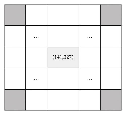
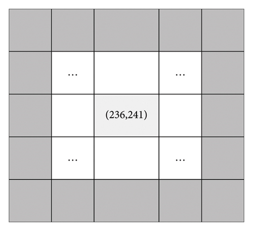
The mathematical model of this problem is converted into a CPLEX program to evaluate the correctness of the model and algorithm. The experimental test data are Set1, a small-scale test data set that IBM ILOG CPLEX12.8 can solve. In the Set1 data, the maximum flight time is under 1 hour [09:00–10:00]. The arrival time to the destination node must be before 10:00. The city (141,327) was chosen as the starting point, and the four vertices of a square extending outward from the starting point were chosen as the destination points. A total of 5 days of data were selected, and the destination points in each data were successively chosen from 1 unit distance outward to 5 unit distances. So this will have 25 test cases in the Set1 data. The spatial distribution of the start and destination points is shown in Figure 12. The four vertices of the square marked with a gray grid are the destination points. Each case has 4 UAVs.
This paper sets the maximum computing time of CPLEX and the multistage dynamic optimization algorithm to 5 min. If the calculation is not completed within 5 min, both programs will terminate and give the current optimal solution. Then, the experimental analysis is carried out by comparing the calculation results of CPLEX and the algorithm. The data information and calculation results of Set1 data are summarized in Table 2.
| ID | Extending outward value | Day | Minimum x value | Minimum y value | Maximum x value | Maximum y value | CPLEX | Dynamic optimization | ||
|---|---|---|---|---|---|---|---|---|---|---|
| Time | Result | Time | Result | |||||||
| 1 | 1 | 1 | 139 | 325 | 143 | 329 | 0.416 | 16 | 0.31 | 16 |
| 2 | 1 | 2 | 139 | 325 | 143 | 329 | 0.483 | 16 | 0.03 | 16 |
| 3 | 1 | 3 | 139 | 325 | 143 | 329 | 0.109 | 16 | 0.02 | 16 |
| 4 | 1 | 4 | 139 | 325 | 143 | 329 | 0.144 | 16 | 0.05 | 16 |
| 5 | 1 | 5 | 139 | 325 | 143 | 329 | 0.491 | 16 | 0.13 | 16 |
| 6 | 2 | 1 | 138 | 324 | 144 | 330 | 1.472 | 32 | 0.09 | 32 |
| 7 | 2 | 2 | 138 | 324 | 144 | 330 | 0.514 | 32 | 1.11 | 32 |
| 8 | 2 | 3 | 138 | 324 | 144 | 330 | 0.619 | 32 | 0.08 | 32 |
| 9 | 2 | 4 | 138 | 324 | 144 | 330 | 0.518 | 32 | 0.14 | 32 |
| 10 | 2 | 5 | 138 | 324 | 144 | 330 | 0.501 | 32 | 0.14 | 32 |
| 11 | 3 | 1 | 137 | 323 | 145 | 331 | 1.922 | 48 | 0.03 | 48 |
| 12 | 3 | 2 | 137 | 323 | 145 | 331 | 1.592 | 48 | 0.04 | 48 |
| 13 | 3 | 3 | 137 | 323 | 145 | 331 | 2.031 | 48 | 0.03 | 48 |
| 14 | 3 | 4 | 137 | 323 | 145 | 331 | 1.638 | 48 | 0.04 | 48 |
| 15 | 3 | 5 | 137 | 323 | 145 | 331 | 2.172 | 48 | 0.02 | 48 |
| 16 | 4 | 1 | 136 | 322 | 146 | 332 | 5.583 | 64 | 0.1 | 64 |
| 17 | 4 | 2 | 136 | 322 | 146 | 332 | 6.878 | 64 | 0.11 | 64 |
| 18 | 4 | 3 | 136 | 322 | 146 | 332 | 7.125 | 64 | 0.11 | 64 |
| 19 | 4 | 4 | 136 | 322 | 146 | 332 | 5.6 | 64 | 0.06 | 64 |
| 20 | 4 | 5 | 136 | 322 | 146 | 332 | 7.392 | 64 | 0.09 | 64 |
| 21 | 5 | 1 | 135 | 321 | 147 | 333 | 18.97 | 80 | 0.53 | 80 |
| 22 | 5 | 2 | 135 | 321 | 147 | 333 | 19.87 | 80 | 0.08 | 80 |
| 23 | 5 | 3 | 135 | 321 | 147 | 333 | 18.08 | 80 | 0.08 | 80 |
| 24 | 5 | 4 | 135 | 321 | 147 | 333 | 17.97 | 80 | 0.11 | 80 |
| 25 | 5 | 5 | 135 | 321 | 147 | 333 | 18.02 | 80 | 0.08 | 80 |
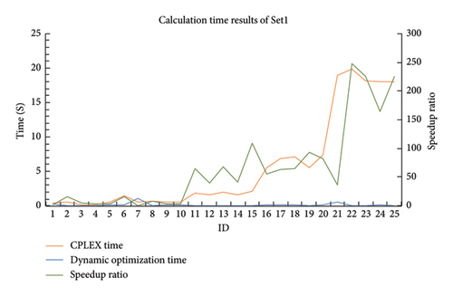
Table 2 shows that the CPLEX results of the mathematical model are generally consistent with the algorithm’s results, which verify the correctness of the dynamic optimization algorithm. As shown in Figure 13, when the scale of the problem grows larger, the calculation time of CPLEX will increase accordingly. The average CPLEX calculation time is 5.6 s. However, the dynamic optimization algorithm is efficient and stable in small-scale examples. Its calculation time is 0.144 s, which is 38.8 times faster than the CPLEX time. Especially, when the problem size becomes larger, the difference in calculation time becomes larger and larger, and the maximum difference can be 248 times. This is because the CPLEX solver uses a general mathematical method to solve the problem. When the problem size becomes larger, the decision variables and constraints increase exponentially and the calculation time becomes longer. However, the algorithm is specifically designed for this problem, reducing a large amount of ineffective calculations, such as some invalid path searches. Therefore, it can solve larger-scale problems more efficiently than the solver. To assess whether the experimental results were statistically significant, a paired-sample t-test was performed on the calculation time, with the results being t = 3.8922 and p = 0.0006. This shows that there is a significant difference in the average computing performance between them at the set significance level α = 0.05. Statistical analysis shows that the algorithm has better average computing performance than CPLEX when using the same data set.
5.3. Effectiveness Validation and Analysis
To verify and analyze the effectiveness of the multistage dynamic optimization algorithm, the large-scale test data set Set2 was used for this experiment. At the same time, to verify the algorithm’s effectiveness, the shortest path A∗ algorithm and Dijkstra algorithm applicable to this problem are implemented in this paper, and comparative testing and experimental analysis are carried out. The Set2 data pick the city (236,241) as the starting point, and all vertices on the edge of a square extending outward from the starting point were chosen as the destination points. In the Set2 data, the maximum flight time is under 7 hours [09:00–16:00]. The arrival to the destination node must be before 16:00. Similarly, a total of 5 days of data were selected, and the destination points in each data were successively chosen from 5 unit distances outward to 25 unit distances with an interval of 5 units each time. So this will also have 25 test cases in the Set2 data. The spatial distribution of the start and destination points is shown in Figure 14. The vertices of the square marked with a gray grid are the destination points. Among them, the largest test case has 200 UAVs.
The shortest path A∗ algorithm is one of the vital heuristic algorithms, which is realized by the estimation function F = GW + HW, which GW represents the cost from the path point to the starting point and HW represents the Manhattan distance from the path point to the endpoint. The shortest path Dijkstra algorithm is one of the most classical algorithms, which relies on the graph structure data for breadth-first search to ensure that the value of the current node is optimal for the value of the previous layer. In the experiment, the algorithm flow of solving this problem remains unchanged. The distinction is to replace the CH algorithm with the A∗ and Dijkstra algorithms, respectively, for the comparative test of the shortest path. The data information and calculation results of Set2 data are summarized in Table 3. In Table 3, column “EOV” denotes extending outward value, column “mini_x” denotes minimum x value, column “mini_y” denotes minimum y value, column “max_x” denotes maximum x value, column “mini_x” denotes maximum x value, and column “p” denotes the preprocessing time.
| ID | EOV | Day | mini_x | mini_y | max_x | max_y | Dynamic optimization | A∗ | Dijkstra | ||||
|---|---|---|---|---|---|---|---|---|---|---|---|---|---|
| p | Time | Result | Time | Result | Time | Result | |||||||
| 1 | 5 | 1 | 225 | 230 | 245 | 250 | 1.445 | 0.941 | 57,600 | 0.603 | 57,600 | 1.674 | 57,600 |
| 2 | 5 | 2 | 225 | 230 | 245 | 250 | 0.184 | 0.076 | 57,600 | 0.012 | 57,600 | 0.029 | 57,600 |
| 3 | 5 | 3 | 225 | 230 | 245 | 250 | 3.447 | 0.659 | 600 | 0.734 | 600 | 0.541 | 600 |
| 4 | 5 | 4 | 225 | 230 | 245 | 250 | 0.942 | 0.622 | 57,600 | 1.024 | 57,600 | 0.311 | 57,600 |
| 5 | 5 | 5 | 225 | 230 | 245 | 250 | 1.658 | 0.198 | 57,600 | 0.215 | 57,600 | 0.237 | 57,600 |
| 6 | 10 | 1 | 220 | 225 | 250 | 255 | 42.93 | 4.233 | 115,200 | 18.016 | 115,200 | 16.396 | 115,200 |
| 7 | 10 | 2 | 220 | 225 | 250 | 255 | 2.656 | 1.24 | 115,200 | 0.027 | 115,200 | 0.1 | 115,200 |
| 8 | 10 | 3 | 220 | 225 | 250 | 255 | 71.731 | 4.818 | 2400 | 12.362 | 2400 | 11.614 | 2400 |
| 9 | 10 | 4 | 220 | 225 | 250 | 255 | 6.608 | 2.202 | 115,200 | 7.411 | 115,200 | 6.447 | 115,200 |
| 10 | 10 | 5 | 220 | 225 | 250 | 255 | 47.577 | 2.882 | 115,200 | 8.017 | 115,200 | 7.563 | 115,200 |
| 11 | 15 | 1 | 215 | 220 | 255 | 260 | 222.304 | 49.759 | 48,598 | 374.808 | 48,598 | 351.88 | 48,598 |
| 12 | 15 | 2 | 215 | 220 | 255 | 260 | 62.898 | 7.355 | 172,800 | 4.212 | 172,800 | 4.053 | 172,800 |
| 13 | 15 | 3 | 215 | 220 | 255 | 260 | 399.899 | 22.694 | 5400 | 86.991 | 5400 | 80.731 | 5400 |
| 14 | 15 | 4 | 215 | 220 | 255 | 260 | 73.454 | 174.6 | 172,800 | 570.768 | 172,800 | 535.47 | 172,800 |
| 15 | 15 | 5 | 215 | 220 | 255 | 260 | 337.538 | 20.001 | 172,800 | 66.285 | 172,800 | 59.86 | 172,800 |
| 16 | 20 | 1 | 210 | 215 | 260 | 265 | 586.684 | 1205.5 | 41,810 | 3088.82 | 41,810 | 2937.2 | 41,810 |
| 17 | 20 | 2 | 210 | 215 | 260 | 265 | 410.79 | 44.323 | 230,400 | 106.475 | 230,400 | 98.723 | 230,400 |
| 18 | 20 | 3 | 210 | 215 | 260 | 265 | 1377.93 | 83.165 | 9600 | 363.236 | 9600 | 337.17 | 9600 |
| 19 | 20 | 4 | 210 | 215 | 260 | 265 | 520.997 | 932.54 | 230,400 | 3554.56 | 230,400 | 3329.6 | 230,400 |
| 20 | 20 | 5 | 210 | 215 | 260 | 265 | 1149.06 | 72.325 | 230,400 | 295.245 | 230,400 | 278.34 | 230,400 |
| 21 | 25 | 1 | 205 | 210 | 265 | 270 | 914.294 | 600.68 | 136,492 | 2614.4 | 136,492 | 2482.4 | 136,492 |
| 22 | 25 | 2 | 205 | 210 | 265 | 270 | 933.288 | 59.354 | 288,000 | 201.782 | 288,000 | 189.48 | 288,000 |
| 23 | 25 | 3 | 205 | 210 | 265 | 270 | 3020.13 | 175.04 | 288,000 | 944.048 | 288,000 | 876.94 | 288,000 |
| 24 | 25 | 4 | 205 | 210 | 265 | 270 | 950.447 | 396.35 | 288,000 | 1696.42 | 288,000 | 1586.6 | 288,000 |
| 25 | 25 | 5 | 205 | 210 | 265 | 270 | 2279.05 | 144 | 288,000 | 783.009 | 288,000 | 733.48 | 288,000 |
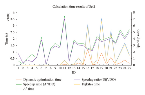
Table 3 and Figure 15 show the multistage dynamic optimization algorithm having an additional preprocessing time, which is very time-consuming and takes an average of 536.7 s. Fortunately, it is a one-time calculation time-consuming, providing efficient services for a large amount of subsequent new calculations or repeated calculations. When the scale of the problem is enlarged, the calculation time of the A∗ and Dijkstra algorithms increases rapidly and changes dramatically. In contrast, the calculation time of the algorithm increases slowly and varies linearly. Without considering the preprocessing time, compared with the A∗ algorithm and Dijkstra algorithm, the dynamic optimization algorithm can calculate the UAV group distribution solution faster. The average calculation time of the A∗ algorithm is 592 s, and the Dijkstra algorithm is 557 s. However, the algorithm takes an average of 160 s, which is 3.69 times faster than A∗ and 3.47 times more than Dijkstra. This can prove that the dynamic optimization algorithm has good solving efficiency and stability in large-scale examples. Because after the algorithm completes the preprocessing process, each subsequent shortest path calculation is almost equivalent to a fast table query, and the time consumption becomes stable and small. However, each shortest path calculation of A∗ and Dijkstra is a completely new calculation and requires continuous querying, inserting, deleting nodes, and comparing weight values. Therefore, when the search network structure is determined, the greater the number of UAV, the better the effect of the dynamic optimization algorithm will be. In order to evaluate whether the experimental results are statistically significant, the three algorithms were grouped in pairs, and each group performed a paired-sample t-test on their computing time. The test results of the algorithm and A∗ are t = −2.9413 and p = 0.0071, the test results of the algorithm and Dijkstra are t = −2.9364 and p = 0.0072, and the test results of A∗ and Dijkstra are t = 2.9747 and p = 0.0065. These show that there is a significant difference in their average computing performance at the set significance level α = 0.05. Statistical analysis shows that when using the same data set, the algorithm has better average computing performance than A∗ and Dijkstra.
A special point to note about this experiment is that the preprocessing time was not considered when calculating the runtime of the proposed algorithm. The experimental result data revealed that when the preprocessing time is taken into account, the proposed algorithm is on average 105 s slower than A∗ and 140 s slower than Dijkstra. However, the preprocessing process is one-time and the resulting data can be used repeatedly. Through the analysis of existing experimental data, it can be found that the preprocessed result data only need to be reused once, and the calculation time of the proposed algorithm (536.7 + 160 ∗ 2 = 856.7) will be less than that of A∗ (592 ∗ 2 = 1184) and Dijkstra (557 ∗ 2 = 1114) that are recalculated twice. As the preprocessed result data are reused more times, the algorithm will save more time. From this perspective, this still proves the effectiveness of the algorithm.
5.4. Parameter Sensitivity Analysis
The proposed method is designed based on a large-scale three-dimensional network structure. The size of the three-dimensional network structure will directly affect the overall calculation amount of the method. Therefore, any parameter that affects the size of the three-dimensional network structure will have an impact on the performance of the proposed method. It is acknowledged that the change in wind speed threshold and rainfall threshold will affect the structure of the network diagram, which will further influence the calculation of the overall algorithm. To analyze the practicability and performance of the algorithm in this paper, the parameter sensitivity analysis is carried out to study the impact of the change of wind speed threshold and rainfall threshold on the algorithm’s performance under different weather threshold conditions. The large-scale test data set Set3 was used for this experiment. In the Set3 data, except for wind speed threshold and rainfall threshold data, the other data information is the same as the Set2 data.
When analyzing the wind speed sensitivity, the rainfall threshold is fixed at 4, and the wind speed threshold ranges from 12.5 to 14.5 at an interval of 0.5. Similarly, a total of 5 days of data were selected. So there are 25 test cases for this experiment on wind speed sensitivity. The data information and calculation results of the Set3 data for wind speed sensitivity analysis are shown in Table 4. In Table 4, column “edge num” denotes the total edge number of the space–time network.
| ID | EOV | Day | mini_x | mini_y | max_x | max_y | Wind speed | Rainfall | Edge num | Dynamic optimization algorithm | ||
|---|---|---|---|---|---|---|---|---|---|---|---|---|
| p | Time | Result | ||||||||||
| 1 | 25 | 1 | 205 | 210 | 265 | 270 | 12.5 | 4 | 1,348,401 | 413.722 | 269.936 | 154,088 |
| 2 | 25 | 1 | 205 | 210 | 265 | 270 | 13 | 4 | 1,571,414 | 592.583 | 499.743 | 145,962 |
| 3 | 25 | 1 | 205 | 210 | 265 | 270 | 13.5 | 4 | 1,722,978 | 759.77 | 691.698 | 136,492 |
| 4 | 25 | 1 | 205 | 210 | 265 | 270 | 14 | 4 | 1,812,828 | 811.043 | 792.262 | 136,492 |
| 5 | 25 | 1 | 205 | 210 | 265 | 270 | 14.5 | 4 | 1,882,341 | 959.051 | 839.498 | 136,492 |
| 6 | 25 | 2 | 205 | 210 | 265 | 270 | 12.5 | 4 | 697,976 | 152.829 | 14.295 | 288,000 |
| 7 | 25 | 2 | 205 | 210 | 265 | 270 | 13 | 4 | 898,909 | 234.921 | 49.655 | 288,000 |
| 8 | 25 | 2 | 205 | 210 | 265 | 270 | 13.5 | 4 | 1,099,980 | 292.969 | 68.411 | 288,000 |
| 9 | 25 | 2 | 205 | 210 | 265 | 270 | 14 | 4 | 1,313,053 | 435.354 | 107.346 | 288,000 |
| 10 | 25 | 2 | 205 | 210 | 265 | 270 | 14.5 | 4 | 1,522,460 | 636.6 | 122.602 | 288,000 |
| 11 | 25 | 3 | 205 | 210 | 265 | 270 | 12.5 | 4 | 2,718,045 | 3043.14 | 174.513 | 288,000 |
| 12 | 25 | 3 | 205 | 210 | 265 | 270 | 13 | 4 | 2,718,045 | 3061.796 | 171.418 | 288,000 |
| 13 | 25 | 3 | 205 | 210 | 265 | 270 | 13.5 | 4 | 2,718,045 | 3096.809 | 171.311 | 288,000 |
| 14 | 25 | 3 | 205 | 210 | 265 | 270 | 14 | 4 | 2,718,045 | 3069.376 | 173.173 | 288,000 |
| 15 | 25 | 3 | 205 | 210 | 265 | 270 | 14.5 | 4 | 2,718,045 | 3078.328 | 169.971 | 288,000 |
| 16 | 25 | 4 | 205 | 210 | 265 | 270 | 12.5 | 4 | 939,867 | 236.913 | 77.062 | 288,000 |
| 17 | 25 | 4 | 205 | 210 | 265 | 270 | 13 | 4 | 1,178,616 | 336.744 | 113.001 | 288,000 |
| 18 | 25 | 4 | 205 | 210 | 265 | 270 | 13.5 | 4 | 1,399,964 | 556.683 | 139.759 | 288,000 |
| 19 | 25 | 4 | 205 | 210 | 265 | 270 | 14 | 4 | 1,579,826 | 644.72 | 194.015 | 288,000 |
| 20 | 25 | 4 | 205 | 210 | 265 | 270 | 14.5 | 4 | 1,734,367 | 809.007 | 285.962 | 288,000 |
| 21 | 25 | 5 | 205 | 210 | 265 | 270 | 12.5 | 4 | 2,269,708 | 1876.697 | 186.72 | 288,000 |
| 22 | 25 | 5 | 205 | 210 | 265 | 270 | 13 | 4 | 2,355,242 | 1855.666 | 133.23 | 288,000 |
| 23 | 25 | 5 | 205 | 210 | 265 | 270 | 13.5 | 4 | 2,400,284 | 2031.332 | 136.986 | 288,000 |
| 24 | 25 | 5 | 205 | 210 | 265 | 270 | 14 | 4 | 2,438,310 | 2276.597 | 139.321 | 288,000 |
| 25 | 25 | 5 | 205 | 210 | 265 | 270 | 14.5 | 4 | 2,476,878 | 2081.369 | 142.473 | 288,000 |
- Note: The current experiment is to do a sensitivity analysis of wind speed, so the changes in wind speed values are marked in bold font.
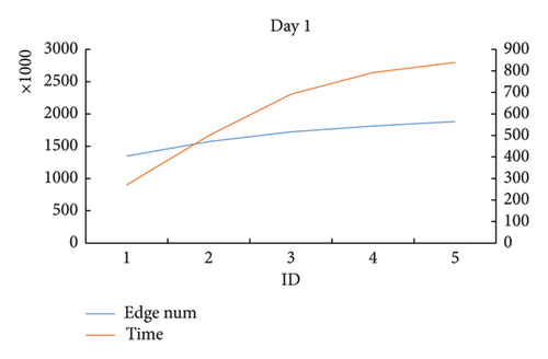
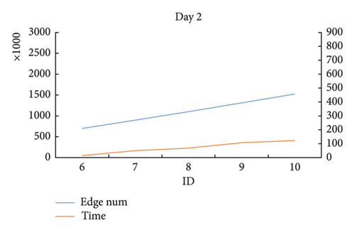
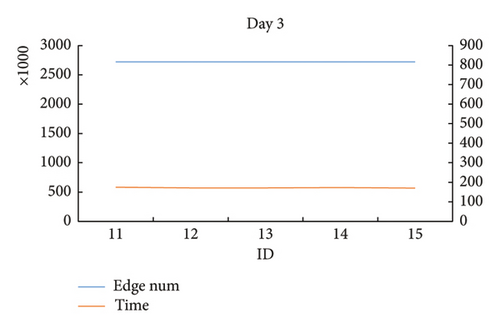
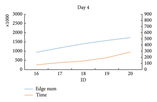
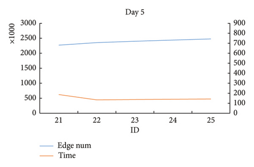
From the result data of Table 4 and Figure 16, it is found that in some test cases on the same day, when the threshold of wind speed gradually increased, the size of the network structure gradually increased, and the calculation time of the proposed algorithm increased accordingly. At the same time, there are some test cases on the same day showing that when the wind speed threshold gradually increases, the size of the network structures changes a little. And the calculation time of the proposed algorithm accordingly remains relatively stable.
When analyzing the rainfall sensitivity, the wind speed threshold is fixed at 15, and the rainfall threshold ranges from 1.5 to 3.5 at an interval of 0.5. Similarly, a total of 5 days of data were selected. So there are 25 test cases for this experiment on rainfall sensitivity. The data information and calculation results of the Set3 data for rainfall sensitivity analysis are shown in Table 5. In Table 5, column “edge num” denotes the total edge number of the space–time network.
| ID | EOV | Day | mini_x | mini_y | max_x | max_y | Wind speed | Rainfall | Edge num | Dynamic optimization algorithm | ||
|---|---|---|---|---|---|---|---|---|---|---|---|---|
| p | Time | Result | ||||||||||
| 1 | 25 | 1 | 205 | 210 | 265 | 270 | 15 | 1.5 | 566,737 | 40.635 | 59.069 | 288,000 |
| 2 | 25 | 1 | 205 | 210 | 265 | 270 | 15 | 2 | 945,968 | 117.196 | 371.396 | 277,248 |
| 3 | 25 | 1 | 205 | 210 | 265 | 270 | 15 | 2.5 | 1,323,010 | 401.741 | 654.539 | 248,370 |
| 4 | 25 | 1 | 205 | 210 | 265 | 270 | 15 | 3 | 1,605,667 | 682.319 | 509.893 | 180,156 |
| 5 | 25 | 1 | 205 | 210 | 265 | 270 | 15 | 3.5 | 1,786,634 | 841.92 | 623.302 | 159,712 |
| 6 | 25 | 2 | 205 | 210 | 265 | 270 | 15 | 1.5 | 1,742,579 | 918.75 | 57.792 | 288,000 |
| 7 | 25 | 2 | 205 | 210 | 265 | 270 | 15 | 2 | 1,742,579 | 927.434 | 58.075 | 288,000 |
| 8 | 25 | 2 | 205 | 210 | 265 | 270 | 15 | 2.5 | 1,742,579 | 934.404 | 57.193 | 288,000 |
| 9 | 25 | 2 | 205 | 210 | 265 | 270 | 15 | 3 | 1,742,579 | 915.133 | 57.684 | 288,000 |
| 10 | 25 | 2 | 205 | 210 | 265 | 270 | 15 | 3.5 | 1,742,579 | 914.398 | 57.795 | 288,000 |
| 11 | 25 | 3 | 205 | 210 | 265 | 270 | 15 | 1.5 | 2,718,045 | 3035.66 | 167.681 | 288,000 |
| 12 | 25 | 3 | 205 | 210 | 265 | 270 | 15 | 2 | 2,718,045 | 3104.285 | 170.6 | 288,000 |
| 13 | 25 | 3 | 205 | 210 | 265 | 270 | 15 | 2.5 | 2,718,045 | 3010.39 | 168.767 | 288,000 |
| 14 | 25 | 3 | 205 | 210 | 265 | 270 | 15 | 3 | 2,718,045 | 3021.237 | 169.767 | 288,000 |
| 15 | 25 | 3 | 205 | 210 | 265 | 270 | 15 | 3.5 | 2,718,045 | 3014.482 | 172.17 | 288,000 |
| 16 | 25 | 4 | 205 | 210 | 265 | 270 | 15 | 1.5 | 1,891,174 | 948.986 | 381.934 | 288,000 |
| 17 | 25 | 4 | 205 | 210 | 265 | 270 | 15 | 2 | 1,891,174 | 945.959 | 381.544 | 288,000 |
| 18 | 25 | 4 | 205 | 210 | 265 | 270 | 15 | 2.5 | 1,891,174 | 950.703 | 382.759 | 288,000 |
| 19 | 25 | 4 | 205 | 210 | 265 | 270 | 15 | 3 | 1,891,174 | 958.57 | 379.728 | 288,000 |
| 20 | 25 | 4 | 205 | 210 | 265 | 270 | 15 | 3.5 | 1,891,174 | 933.513 | 379.385 | 288,000 |
| 21 | 25 | 5 | 205 | 210 | 265 | 270 | 15 | 1.5 | 2,286,412 | 2077.473 | 171.052 | 288,000 |
| 22 | 25 | 5 | 205 | 210 | 265 | 270 | 15 | 2 | 2,413,376 | 1919.127 | 196.646 | 288,000 |
| 23 | 25 | 5 | 205 | 210 | 265 | 270 | 15 | 2.5 | 2,484,919 | 2098.679 | 232.068 | 288,000 |
| 24 | 25 | 5 | 205 | 210 | 265 | 270 | 15 | 3 | 2,506,770 | 2180.183 | 149.917 | 288,000 |
| 25 | 25 | 5 | 205 | 210 | 265 | 270 | 15 | 3.5 | 2,511,009 | 2136.953 | 142.004 | 288,000 |
- Note: The current experiment is to do a sensitivity analysis of rainfall, so the changes in rainfall values are marked in bold font.
From the result data of Table 5 and Figure 17, similar conclusions were found regarding the sensitivity to wind speed as those observed in the above experiments. The calculation time of the proposed method is positively related to the scale of the network structure. When the scale of the network structure becomes larger, the calculation time becomes longer. Likewise, when the size of the network structure changes slightly, the computation time does not change much.
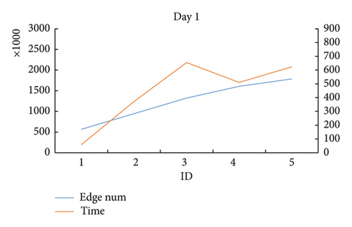
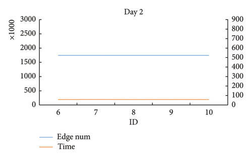
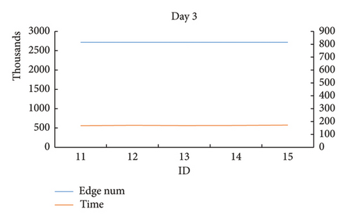
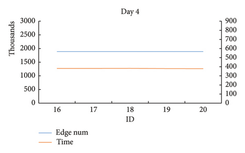
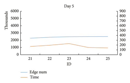
It can be concluded from Figures 16 and 17 that the size of the network structure shows a strong positive correlation with the calculation time of the algorithm. When the scale of the network structure changes with the wind speed threshold and rainfall threshold, the calculation time of dynamic optimization calculation also changes, and there are no obvious abnormal fluctuations. When the wind speed threshold and rainfall threshold exceed specific values, there is no area where UAVs cannot fly and no change in the size of the network structure, and the corresponding calculation time tends to be stable. It turns out that the solving efficiency and stability of the dynamic optimization algorithm are strongly related to the size of the network structure, and the size of the network structure is strongly related to the wind speed threshold and rainfall threshold. Therefore, the performance of the proposed algorithm can be affected by adjusting the wind speed threshold and rainfall threshold. A feasible and safer solution can be found more quickly by lowering the wind speed threshold and rainfall threshold. The relationship between the specific sizes of these thresholds and the size of the network structure can be obtained through advanced data preprocessing operations.
6. Conclusion
UAVs conform to the development trend of the times and have gradually been widely valued, applied, and studied in logistics distribution services. Since UAVs will be affected by different safety factors such as rainfall and wind speed at different times and spaces in practical applications, this paper studies the optimization problem of UAV group distribution routes under a time-varying weather network. The corresponding mathematical model of the problem is established. In addition, this paper proposed a multistage dynamic optimization algorithm for seeking the optimal solution due to the issue having the characteristics of a large-scale and variable space–time network and a safe take-off time interval limitation between UAVs. Finally, based on the actual case data, this paper verifies the accuracy of the mathematical model and the algorithm’s effectiveness, proving the algorithm’s stability and the particular application value it possesses.
The proposed work is for planners who make UAV delivery plans. It does not require high timeliness and only requires repeated attempts and modifications to finally output the plan within a few hours. However, this also has two limitations. First, the model does not consider the impact of uncertain changes in future weather data on the feasibility of the flight route. Second, the algorithm is not suitable for quickly calculating a new version of the adjustment plan under recent changes in data. In the future, the author will carry out more in-depth research based on this paper. Looking ahead, prospects for this research include developing advanced predictive models that can dynamically adjust to uncertain and changing weather conditions and enhancing the UAV distribution route planning under such variability. Additionally, the creation of more sophisticated algorithms capable of rapid reoptimization could significantly improve responsiveness to real-time data updates, making the planning process more agile and better suited for time-critical applications. Another avenue for exploration could be the integration of artificial intelligence and machine learning techniques to further refine the decision-making process, potentially allowing for more accurate weather predictions and adaptive route adjustments. Finally, there is potential for expanding the applicability of the model to other areas of UAV operation, such as emergency response or surveillance, where the ability to swiftly adapt to changing conditions is paramount.
Conflicts of Interest
The authors declare no conflicts of interest.
Author Contributions
Wanchen Jie (conceptualization, methodology, writing–original draft, writing–review and editing): mainly responsible for the conception and design of the study, data acquisition, data analysis and interpretation, and drafting the first draft. She was also instrumental in revising the manuscript for important content.
Cheng Pei (data curation, software, formal analysis, visualization, investigation): made significant contributions to the study’s methodological design and implementation, experimental design, data collection, and interpretation of experimental results. He assisted in drafting the manuscript and also maintained good communication with the editorial office as the corresponding author.
Hong Yan (funding acquisition, project administration, supervision): as senior author and research supervisor, participated in the conceptualization of the initial ideas and supervised the execution of the project. He provided guidance throughout the research process and provided funding and resources needed for the research.
Weitong Lin (resources, validation): provided specific technical expertise in statistical analysis and contributed to the interpretation of the data. In particular, he critically revised the Results and Discussion sections of the manuscript.
Funding
This work was supported by Youth Project of the National Natural Science Foundation of China (71901192) and Talent Person Recruitment Project of Zhejiang Shuren University (KXJ0121604).
Open Research
Data Availability Statement
This experiment is based on the desensitized predicted meteorological data from the British Meteorological Office. The data include location coordinate information, weather time, wind speed, and rainfall. Some of the most important weather datasets produced by the Met Office are now available for free on Amazon Web Services. The GitHub repository (https://github.com/MetOffice/aws-earth-examples) contains example code of how to access these datasets.


