Software Defect Prediction Based on Fuzzy Cost Broad Learning System
Abstract
Software defect prediction (SDP) is an effective approach to ensure software reliability. Machine learning models have been widely employed in SDP, but they ignore the impact of class imbalance, noise and outliers on the prediction performance. This study proposes a fuzzy cost broad learning system (FC-BLS). FC-BLS not only handles class imbalance problems but also considers the specific sample distribution to address noise and outliers in software defect datasets. Our approach draws fully on the idea of the cost matrix and fuzzy membership functions. It introduces them to BLS, where the cost matrix prioritises the training errors on the minority samples. Hence, the classification hyperplane position is more reasonable, and fuzzy membership functions calculate the membership degree of the sample in a feature mapping space to remove the prediction error caused by noise and outlier samples. Then, the optimisation problem is constructed based on the idea that the minority class and normal instances have relatively high costs. By contrast, the majority class and noise and outlier instances have relatively small costs. This study conducted experiments on nine NASA SDP datasets, and the experimental findings demonstrated the effectiveness of the proposed methodology on most datasets.
1. Introduction
As software engineering continues to develop, research on software defects has gradually become a prominent topic in the field of software reliability [1], making software defect prediction (SDP) one of the fastest-growing and most significant technologies. The SDP technology is designed to predict modules in software systems that are susceptible to defects, thereby allocating testing resources more effectively [2]. Consequently, an effective SDP can lead to cost savings in testing, enhance software quality [3] and positively affect human beings and society [4].
In our previous studies [5, 6], we investigated the phenomenon of class overlap, where defective and nondefective samples exhibited similarities in metric values, and assessed its influence on SDP performance. Additionally, we addressed class imbalance in both within-project and cross-project scenarios by proposing a method called STr-NN, with experimental results demonstrating its effectiveness. Moreover, studying the influence of classification techniques on SDP performance is crucial. Therefore, a novel classification technique suitable for SDP is required.
Currently, machine learning, such as nearest neighbour [7], support vector machine (SVM) [8], neural network [9], logistic regression [10], ensemble methods [11, 12] and extreme learning machine (ELM) [13], is the primary classification technology in traditional SDP [14, 15]. The primary processes included data collection, data processing, model training and model evaluation. Moreover, many variants of machine learning models have been used to improve the accuracy of SDP. For example, Zada et al. [16] combined the war strategy optimisation (WSO) algorithm and kernel extreme learning machine (KELM) for SDP to optimise classifier hyperparameters and consequently elevate defect detection efficiency within software components. However, owing to the nonlinear separability of SDP data, traditional classification algorithms often struggle to adequately represent high-dimensional and sparse software defect data, leading to underfitting. Therefore, many deep learning methods have been utilised in SDP. Unlike conventional machine learning, deep learning possesses the ability to automatically learn and extract discriminative features from data, leading to the creation of a more accurate SDP model. For instance, Šikić et al. [17] utilised a convolutional graph neural network (GCNN) as the underlying framework to obtain characteristics from an Abstract Syntax Tree to improve the classification performance. Chakraborty and Chakraborty [18] presented a deep feedforward neural network with an internal hierarchy, namely the Hellinger net, and it utilised a stochastic gradient descent backpropagation algorithm for training the model.
Despite the excellent capability of deep learning methods to represent data features, most methods exhibit a significant number of parameters and complex structures. The training process of these models usually entails layer-wise unsupervised pre-training and overall supervised fine-tuning, making the model optimisation process cumbersome. Moreover, deep learning models involve solving highly nonconvex optimisation problems, making it challenging to conduct a theoretical analysis of deep architectures. Currently, most efforts are focused on tuning parameters or adding more layers to enhance accuracy. To alleviate the challenges above, Chen and Liu [19] proposed a broad learning system (BLS) that extends neurones in a broad manner, rather than being confined to deep stacked layers. The output weights are then computed using a pseudoinverse. Compared to popular deep learning models, BLS can handle large-scale data and can be applied to incremental learning models without retraining the entire model when adding new nodes.
In conclusion, BLS was utilised as the fundamental classifier for SDP owing to its structural simplicity, few training parameters and rapid training. Nevertheless, conventional BLS cannot address the effects of class imbalances, outliers and noise that may be present in datasets. Class imbalance can cause a BLS to overlook potentially more valuable minority classes, owing to its widespread application. Noise and outliers were also present in the software defect data. Certain training points were affected by noise, resulting in data corruption. In addition, BLS may overfit the outliers, thereby affecting the classification results for normal data. Conventional BLS relies primarily on the distinguishability of different sample classes, sometimes overlooking variations in sample quantities across different classes and the special sample distribution in the feature space.
- 1.
We propose a new variant of the BLS, namely, FC-BLS. This model improves the loss function of BLS by employing cost matrix strategies and fuzzy membership functions to address class imbalances and simultaneously mitigate outliers and noise.
- 2.
The cost matrix is leveraged to solve the class imbalance. The cost matrix prioritises the training errors on the minority samples, making the classification hyperplane position more reasonable. Higher costs are assigned to defective modules to emphasise the importance of minority classes in solving class imbalance problems.
- 3.
A fuzzy membership function addresses noise and outliers. The fuzzy membership function considers the specific sample distribution in feature space. It calculates the class centres of all samples in the same class, the radius of all samples and the distance from the samples to the class centres using clustering and K neighbours. Thus a fuzzy membership function is designed, in which a higher degree of membership indicates a stronger influence of that data point on the model.
The remainder of this paper is organised as follows. Section 2 provides prior knowledge relevant to SDP work. Section 3 presents a comprehensive description of the proposed method. The experimental setup is outlined in Section 4. Section 5 presents the experimental results and analyses. Finally, Section 6 concludes the study.
2. Related Work
2.1. Class Imbalanced Learning for Defect Prediction
Various approaches have been proposed at the data and algorithm levels to tackle class imbalance issue in the SDP [20]. Data-level methods employ re-sampling techniques, which are the preprocessing techniques, and adjust the data distribution to address imbalanced datasets, including oversampling [21, 22], and undersampling techniques [23] to tackle the problem. Stradowski [15] aimed to analyse the state-of-the-art SDP approach by machine learning technology and to identify the new trends in this field. In the case of oversampling, instances from minority classes are duplicated. However, distinguishing whether the replicated instances are beneficial or redundant is challenging, which can render oversampling results unreliable. Oversampling may lead to multiple duplicate samples in the dataset, which may appear overfitting [24]. Chawla et al. [22] proposed the SMOTE, which yields synthetic instances for the minority class to preprocess imbalanced data. Many researchers have proposed different variants of the SMOTE to address class imbalance problems. Torgo et al. [21] proposed an oversampling technique called SmoteR for solving regression problems. Douzas, Bacao and Last [25] presented K-means SMOTE to balance samples. Improved oversampling techniques were also proposed. Yedida and Menzies [26] introduced a fuzzy oversampling method to enhance the efficacy of deep learning on imbalanced datasets. Arun and Lakshmi [27] introduced a multicluster-based oversampling method to address the class imbalance and smaller disjuncts effectively. Wang, Liu and Bai [28] introduced an enhanced defect prediction approach that incorporates oversampling techniques to effectively mitigate class imbalance, class overlap and noise issues. These sophisticated oversampling techniques, while enhancing the diversity and representativeness of synthetic samples, continue to face challenges in determining the optimal number of synthetic instances and ensuring their alignment with the underlying data distribution, potentially limiting their applicability in SDP. Unlike oversampling approaches, undersampling techniques attain balance by reducing the number of instances in the majority class. However, it can be challenging to determine whether the deleted instances are redundant or beneficial, which results in the loss of instance information [29]. Khoshgoftar et al. [30, 31] employed a random undersampling (RUS) technique for imbalanced data. Furthermore, some researchers have suggested methods that combine undersampling and oversampling to mitigate imbalanced sample issues [32, 33].
At the algorithmic level, ensemble learning and cost-sensitive (CS) learning are frequently employed to tackle class imbalance. Bagging and boosting in ensemble learning have proven effective [34]. Wang and Yao [35] analysed the proposed ensemble method, DNC (Dynamic Adabort.NC), and found it to outperform ROS, RUS and SMOTE. Tang et al. [36] employed bagging ensemble learning in conjunction with the adaptive variable sparrow search algorithm ELM to mitigate dataset imbalance; however, the parameter selection process of this algorithm resulted in increased time overhead. CS learning allocates a significant penalty for misclassifying samples from the minority class while assigning a comparatively lower cost to misclassifying samples from the majority class. Khoshgotaar et al. [37] introduced a cost-boosting approach incorporating CS learning into SDP. Zheng [38] studied the efficacy of CS-boosting algorithms for augmenting neural networks. Arar and Ayan [39] conducted research on CS neural networks. Jin [40] considered intersample relationships and subsequently utilised CS learning to enhance distance metric learning to achieve sample balance. In summary, the CS algorithm can set the cost weights of different categories to adjust the model’s attention to different categories, making it more flexible and improving its generalisation performance.
2.2. BLS
The BLS can overcome the challenge of prolonged training processes in deep learning by expanding the width of the neural network. Moreover, BLS can reduce the time required to construct a network model. The input data are initially mapped into mapped nodes via BLS and subsequently enhanced to the enhancement nodes. Then, all the nodes are jointly input into the hidden layer. Finally, we use the pseudoinverse to calculate the weight that connects the hidden and output layers. In cases where the nodes are insufficient, the BLS eliminates the need to initiate the learning process from scratch. Instead, it simply adjusts the weights related to the added nodes to facilitate rapid retraining. Since its proposal, BLS has found extensive applications in diverse fields, including human activity recognition [41], feature extraction using the K-means clustering algorithm [42], multimodal information fusion in BLS [43], image classification [44], artificial intelligence [45] and imbalanced data classification [46]. This demonstrates that BLS exhibits robustness, generalisation ability and scalability.
3. Proposed Model
In this section, the FC-BLS introduces the cost matrix and fuzzy membership function into the BLS respectively to reduce the influence of class imbalance, noise and outliers on the prediction accuracy. The procedure for prediction using FC-BLS is depicted in Figure 1.
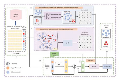
FC-BLS mainly consists of three parts: (1) BLS model: the fundamental classifier of FC-BLS, enhancing the prediction process under its simplistic structure and low training parameters; (2) cost matrix: making the minority class obtain a more significant cost, and adding it to the BLS, hence increasing the sensitivity of the classifier towards the minority class and solving the issue of effective classification of imbalanced samples; (3) fuzzy membership function: considering the sample’s distribution in feature space, as well as the influence of noise and outliers, calculating the membership degree of the sample in the feature mapping space, and adding it to the BLS to eliminate the prediction error caused by noise and outlier samples, which significantly improve BLS, the classification effectiveness and generalisation ability.
3.1. BLS Model
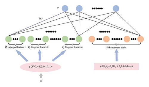
BLS uses both n groups of mapped nodes and m groups of enhancement nodes as inputs to the hidden layer, and each group of mapped and enhancement nodes contains N and M neural nodes, respectively, and b is the dimensionality of the output data. The BLS model structure is depicted in Figure 2.
Here, λ is the regularisation parameter.
3.2. Design of Cost Matrix
3.3. Design of Fuzzy Membership Functions
In equations (12) and (13), we made σ > 0, δ > 0 and to avoid si = 0 and ηi = 0.
3.4. FC-BLS Model
Here, Q = TC, the membership degree matrix T = diag(ti), i = 1, 2, …, L and the cost matrix C = diag(cii), i = 1, 2, …, L
3.5. Computational Complexity Analysis
4. Experimental Setup
This section introduces the software defect datasets and performance evaluation metrics employed in this experiment. Finally, the experimental setup and procedures are described.
4.1. Software Defect Dataset
All experimental datasets were based on NASA datasets. Table 1 provides the characteristics of the datasets. Notably, owing to the imbalance rates ranging from 2.1% to 35.2% across all datasets, each dataset exhibited class imbalance problem.
| Datasets | Number of instances | Number of metrics | Defective (%) |
|---|---|---|---|
| CM1 | 327 | 37 | 12.8 |
| KC3 | 194 | 39 | 18.6 |
| MC2 | 125 | 39 | 35.2 |
| MW1 | 253 | 37 | 10.7 |
| PC1 | 705 | 37 | 8.7 |
| PC2 | 745 | 36 | 2.1 |
| PC3 | 1077 | 37 | 12.4 |
| PC4 | 1287 | 37 | 13.8 |
| PC5 | 1711 | 38 | 27.5 |
4.2. Performance Indicators
In the scenario of imbalanced SDP datasets, we utilised the F-measure, AUC and Recall as performance indicators. These indicators also assess whether the proposed method effectively balances the majority and minority classes. Table 2 shows the confusion matrix and the Recall, Precision and F-measure defined using the confusion matrix. The Recall is the proportion of samples that correctly predicted to be defective among all defective samples. The F-measure is the weighted harmonic average of the Precision and Recall. The AUC is often utilised to gauge the model’s ability to balance performance between two classes [47]. The higher the value of the F-measure, AUC and recall, the better the classification effect of the FC-BLS.
| Predicted as defective | Predicted as nondefective | |
|---|---|---|
| Actual defective | TP | FN |
| Actual nondefective | FP | TN |
| Recall | TP/TP + FN | |
| Precision | TP/TP + FP | |
| F-measure | 2∗recall∗precision/recall + precision | |
4.3. Experimental Design
The experimental design is described in this section. We conducted experiments using a system equipped with 64 GB of RAM, an NVIDIA GPU (model 8server), CUDA Version 11.4, driver Version 470.182 and NVIDIA-SMI Version 470.182. We utilised Anaconda Version 3 and TensorFlow as the backend for the Keras library. Additionally, we used Numpy as a linear algebra library; Pandas and Sklearn for data interpretation; Imblearn, Scipy and Seaborn for sampling methods; and Matplotlib for data visualisation. We conducted the SDP experiments on nine NASA datasets. First, each NASA dataset was randomly divided into a 75:25 ratio, with the training dataset accounting for 75% of the test dataset accounting for 25%. Then, we performed 10-fold cross-validation to choose the optimal parameter configuration for FC-BLS model performance, the range of values for the number of mapped and enhancement nodes are {15, 20, …, 35}, the regularisation parameter λ took values in the range {2−5, 2−4, …, 24}. Finally, we compared the FC-BLS with other cutting-edge methods using performance indicators.
5. Experimental Results and Analysis
In the comparative experiments, we compared FC-BLS with KNN [7], SVM [8], CNN [9], ELM [13], BLS [19] and Hellinger net [18], and the proposed method was the best among all three evaluation metrics. We used the average of 10 experiments as the final experimental result. Section 5.1 analyses the experimental results using evaluation metrics, and Section 5.2 is a parameter analysis of the FC-BLS, investigating the relationship between different parameter and model performance. In addition, we present the analytical and experimental data in the form of charts for a more intuitive representation.
5.1. Experiment Analysis
The Recall, AUC and F-measure for the different classifiers over the nine NASA datasets are listed in Table 3. The most favourable outcomes are emphasised in bold.
| Dataset | Measure | CNN | KNN | ELM | SVM | Hellinger net | BLS | FC-BLS (proposed) |
|---|---|---|---|---|---|---|---|---|
| CM1 | F-measure | 0.818 | 0.867 | 0.777 | 0.826 | 0.865 | 0.857 | 0.894 |
| AUC | 0.672 | 0.389 | 0.381 | 0.473 | 0.706 | 0.591 | 0.713 | |
| Recall | 0.800 | 0.848 | 0.731 | 0.872 | 0.660 | 0.858 | 0.876 | |
| KC3 | F-measure | 0.772 | 0.794 | 0.760 | 0.833 | 0.832 | 0.763 | 0.858 |
| AUC | 0.574 | 0.464 | 0.514 | 0.500 | 0.744 | 0.610 | 0.798 | |
| Recall | 0.796 | 0.816 | 0.786 | 0.714 | 0.600 | 0.761 | 0.853 | |
| MC2 | F-measure | 0.672 | 0.658 | 0.672 | 0.877 | 0.730 | 0.760 | 0.897 |
| AUC | 0.730 | 0.350 | 0.365 | 0.500 | 0.673 | 0.745 | 0.884 | |
| Recall | 0.656 | 0.656 | 0.672 | 0.781 | 0.540 | 0.759 | 0.897 | |
| MW1 | F-measure | 0.772 | 0.813 | 0.780 | 0.906 | 0.902 | 0.792 | 0.876 |
| AUC | 0.500 | 0.592 | 0.533 | 0.500 | 0.790 | 0.609 | 0.811 | |
| Recall | 0.844 | 0.766 | 0.805 | 0.828 | 0.650 | 0.777 | 0.867 | |
| PC1 | F-measure | 0.860 | 0.876 | 0.857 | 0.902 | 0.945 | 0.899 | 0.925 |
| AUC | 0.561 | 0.479 | 0.336 | 0.402 | 0.854 | 0.707 | 0.787 | |
| Recall | 0.823 | 0.881 | 0.827 | 0.924 | 0.870 | 0.889 | 0.921 | |
| PC2 | F-measure | 0.988 | 0.971 | 0.976 | 0.989 | 0.980 | 0.983 | 0.991 |
| AUC | 0.500 | 0.434 | 0.508 | 0.500 | 0.660 | 0.537 | 0.665 | |
| Recall | 0.992 | 0.973 | 0.974 | 0.979 | 0.200 | 0.986 | 0.992 | |
| PC3 | F-measure | 0.824 | 0.823 | 0.806 | 0.786 | 0.907 | 0.843 | 0.889 |
| AUC | 0.500 | 0.424 | 0.510 | 0.488 | 0.835 | 0.650 | 0.769 | |
| Recall | 0.880 | 0.807 | 0.855 | 0.851 | 0.700 | 0.842 | 0.881 | |
| PC4 | F-measure | 0.866 | 0.813 | 0.852 | 0.787 | 0.900 | 0.874 | 0.903 |
| AUC | 0.632 | 0.451 | 0.300 | 0.491 | 0.842 | 0.739 | 0.852 | |
| Recall | 0.859 | 0.830 | 0.848 | 0.852 | 0.820 | 0.870 | 0.895 | |
| PC5 | F-measure | 0.621 | 0.692 | 0.636 | 0.624 | 0.825 | 0.670 | 0.829 |
| AUC | 0.500 | 0.433 | 0.475 | 0.483 | 0.700 | 0.620 | 0.707 | |
| Recall | 0.734 | 0.734 | 0.667 | 0.729 | 0.500 | 0.658 | 0.809 | |
| Average | F-measure | 0.799 | 0.812 | 0.791 | 0.837 | 0.876 | 0.827 | 0.896 |
| AUC | 0.517 | 0.402 | 0.392 | 0.434 | 0.680 | 0.581 | 0.699 | |
| Recall | 0.738 | 0.731 | 0.716 | 0.753 | 0.554 | 0.740 | 0.799 | |
- Note: Bold values indicate the best-performing model values.
The FC-BLS employs linear feature mapping, thus making it comparable to the SVM and ELM models that utilise linear kernel functions. From Table 3 and Figures 3, 4, 5, it is evident that the experimental results of FC-BLS outperformed those of SVM and ELM on the nine datasets. Compared with the SVM, FC-BLS exhibited a higher average F-measure, AUC and Recall, with increases of 7.08%, 61.06% and 6.12%, respectively. Compared with the ELM, FC-BLS demonstrated a significantly higher average F-measure, AUC and Recall, with increases of 13.31%, 78.11% and 11.55%, respectively. This is because these two classification methods use only the original data features and cannot address the class imbalance, noise and outliers of the dataset. However, the SVM aims to maximise the classification interval and determine the decision boundary by selecting support vectors. If the data tended to be completely separated by a hyperplane in the feature space, the performance indicators of the SVM were better for datasets MW1 and PC1.
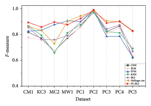

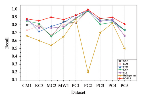
FC-BLS outperformed KNN on all datasets, with a significantly higher average F-measure, AUC and Recall, achieving increases of 13.31%, 78.11% and 11.55%, respectively. KNN classifies the datasets by measuring the distances between different features. However, the average AUC value of KNN is only 0.402, indicating that KNN cannot effectively address the issue of class imbalance. By contrast, FC-BLS yielded significantly superior results.
Compared to CNN, FC-BLS exhibited superior performance across all nine datasets, with notably higher average F-measure, AUC and Recall, achieving increases of 12.11%, 35.18% and 8.23%, respectively. CNN adopts a complex deep learning network structure to determine the optimal parameters and obtain the optimal classification model after a long period of training in multiple iterations. Therefore, CNN obtained the same Recall value on the PC2 dataset as FC-BLS, but CNN was insensitive to a few classes, which did not improve the influence of class imbalance.
The prediction performance of the FC-BLS model surpassed that of the BLS model. FC-BLS exhibited higher average F-measure, AUC and Recall than BLS, with increases of 7.08%, 61.06% and 6.12%, respectively. Therefore, combining the cost matrix and fuzzy membership function is beneficial for improving the classification effect of the SDP.
Compared with Hellinger Net, FC-BLS demonstrated superior performance across all six datasets, with significantly higher average F-measure, AUC and Recall, achieving increases of 2.25%, 2.68% and 44.25%, respectively. The Hellinger net [18] is a deep feedforward neural network with a built-in hierarchy that leverages the robustness of the Hellinger distance, a skew-insensitive distance measure, to address class imbalance effectively. Although Hellinger Net mitigates the issue of class imbalance to some degree, it does not address the challenges posed by noise and outliers in software defect data. However, FC-BLS not only uses the cost matrix to classify imbalanced samples effectively but also considers the specific sample distribution in the feature space and employs the fuzzy membership function to tackle issues related to noise and outliers, which improves the classification effect of SDP.
In summary, FC-BLS outperformed the other comparative methods regarding the three evaluation metrics of F-measure, AUC and Recall on the nine datasets.
5.2. Parametric Analysis
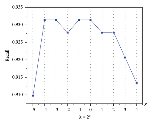
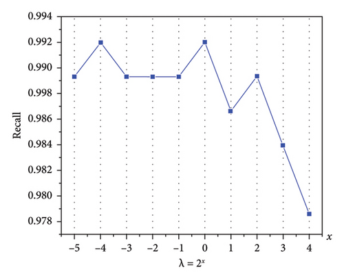
A portion of the weights in FC-BLS was stochastically generated throughout the training procedure. These include the random weights employed in mapping the entry data to the mapping features and utilised in mapping the mapping features to the enhancement nodes. In constructing the optimal model, the experimental outcomes are significantly influenced by the alterations in the quantity of mapped nodes, augmentation nodes and the regularisation parameter λ. The following experiments take three datasets, CM1, PC1 and PC2, as examples, and use Recall as an evaluation metric to analyse the influence of the aforementioned parameters on the prediction efficacy of FC-BLS.
5.2.1. Impact of Mapped Nodes and Enhancement Nodes on Recall
The quantity of mapped and enhancement nodes affected the performance of the FC-BLS model. More mapped nodes result in a higher extraction of a more significant number of features from the mapped features, which is beneficial for improving the Recall. In addition, more enhancement nodes introduce more feature representations and complexity to the FC-BLS, which can enhance the performance and generalisation ability of the model. However, this also requires a more significant amount of computation. Consequently, it is critical to discuss the impact of the quantity of mapped and enhancement nodes on the FC-BLS.
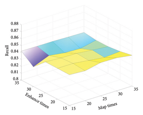
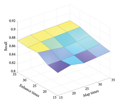
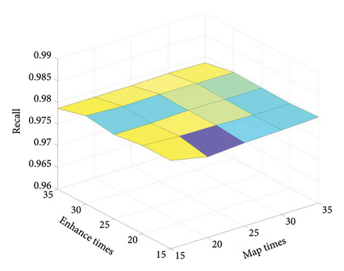
The number of mapped and enhancement nodes take values within a specified range {15, 20, …, 35}, and the regularisation parameter λ = 0.001. The average Recall was obtained after 10 experiments, and the effect of the mapped and enhancement nodes on the Recall is visually depicted in Figure 6. The Recall fluctuates with the quantity of nodes; however, the range between the highest and lowest Recall is minimal, indicating the robust stability of the FC-BLS. On the CM1 dataset, the Recall value is maximum at MapTimes = 25 and EnhanceTimes = 25; on the PC1 dataset, the Recall rises relatively smoothly at MapTimes > 20 and EnhanceTimes > 30, and as the quantity of mapped nodes increases, the computation of FC-BLS increases, the optimal value for MapTimes is 20 and EnhanceTimes is 30; on the PC2 dataset, when MapTimes < 30 and EnhanceTimes < 15, Recall has some fluctuation, but Recall has an overall upward trend. When MapTimes > 30 and EnhanceTimes > 15, the Recall gradually stabilises, and the optimal values of MapTimes and EnhanceTimes are 30 and 15, respectively.
5.2.2. Impact of the Regularisation Parameter λ on Recall
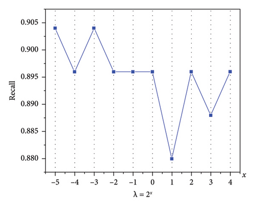
The regularisation parameter is an important BLS hyperparameter that can control the model complexity and avoid overfitting and underfitting phenomena, thus improving the model generalisation ability. If the λ value is excessively small, the model is susceptible to overfitting, whereas an overly large λ value can lead to the underfitting phenomenon. Hence, it is imperative to determine an appropriate value for λ. On the three datasets, λ takes values in the range {2−5, 2−4, …, 24}, and MapTimes = EnhanceTimes = 20. The average Recall is obtained after 10 experiments, and the effect of the regularisation parameter on Recall is depicted in Figure 7. As observed, Recall varies with λ, allowing us to select an optimal value for λ based on these variations.
6. Discussion
Current SDP methods face challenges like class imbalance, noise and outliers, which reduce predictive performance. Traditional models often fail to prioritise minority class samples and are sensitive to noise, leading to distorted decision boundaries. To address these issues, this paper proposes an FC-BLS that uses a cost matrix to emphasise minority class samples and fuzzy membership functions to reduce the impact of noise and outliers. This approach retains the simplicity and fast training of BLSs while improving robustness in complex scenarios. While FC-BLS outperforms traditional methods on multiple NASA datasets, it has limitations. (1) It has only been validated on nine specific datasets, which may limit its generalisability. Its performance is highly sensitive to parameter tuning, increasing training complexity and hindering rapid application to diverse datasets. (2) The performance of FC-BLS is highly sensitive to the number of mapped and enhancement nodes as well as the regularisation parameter λ, with current parameter tuning relying heavily on empirical methods. (3) Although FC-BLS is efficient with large-scale data, its computational complexity may become a bottleneck for extremely large datasets, and it does not effectively handle dynamic or streaming data scenarios, limiting its applicability in real-world software development processes. Future work will focus on expanding datasets, automating parameter tuning, enabling real-time processing and exploring applications in domains like medical diagnosis and financial fraud detection to improve its practical value and contribution to software reliability engineering.
7. Conclusion
We proposed an FC-BLS for SDP, namely the FC-BLS model. We improved the loss function of BLS through constructing a cost matrix and fuzzy membership functions. It improves the class imbalance and considers the specific sample distribution in the feature space to address the noise and outliers in the software defect data. FC-BLS retains the characteristics of the BLS, such as its simple structure and short training time. Incorporation of fuzzy membership functions further enhances the robustness of the model in complex software defect scenarios. We carefully evaluated FC-BLS on nine NASA SDP datasets using three key performance indicators, showing the superior performance of FC-BLS compared to six other methods on most datasets. This study focuses primarily on developing an imbalanced classifier to enhance SDPs on NASA datasets. We may extend this work in the future studies to other SDP scenarios, such as cross-project and semi-supervised scenarios. In the future, we will attempt to utilise the FC-BLS model for data imbalance problems in other fields to prove the generalisation ability of the proposed method.
Conflicts of Interest
The authors declare no conflicts of interest.
Funding
This work was partially supported by grant from the Natural Science Foundation of China (Nos. 62206087, 62276091, 62202223, 61602154), Center for Complexity Science, Henan University of Technology (No. CSKFJJ-2024-7), the Innovative Funds Plan of Henan University of Technology (No. 2022ZKCJ14), Key Laboratory of Grain Information Processing and Control (Henan University of Technology), Ministry of Education (No. KFJJ2024016), Cultivation Programme for Young Backbone Teachers in Henan University of Technology (No. 21420158), General Program of Henan Provincial Natural Science Foundation (No. 242300420279) and National Natural Science Foundation of China Cultivation Project in Henan University of Technology (No. 31490139).
Open Research
Data Availability Statement
The data used to support the findings of this study are included within the article.


