1. Introduction

As industrialization and urbanization progress, the concern regarding urban air pollution has substantially intensified [1, 2]. Consequently, predicting the air quality index has become a crucial focus within the realm of environmental protection. Air quality prediction is regarded as forecasting and estimating concentrations of pollutants in the atmosphere at specific times and locations [3]. This holds significance for public health and safety since exposure to elevated pollutant levels can adversely affect respiratory and cardiovascular health. Air quality prediction models typically integrate data from diverse sources, such as meteorological data, satellite imagery, and ground-level sensors. These models are designed to furnish real-time information on air quality, and forecast air quality levels over an extended duration.

Recent research efforts have focused on enhancing the accuracy and efficiency of air quality prediction models [4–7]. However, traditional prediction models and algorithms often require large amounts of high-quality historical data to achieve optimal performance [8, 9]. The challenge arises from the inconsistency in data availability, as well as the diverse distributions of data from different regions, due to varying factors influencing air quality (e.g., weather, geography, and traffic). These regional and temporal differences lead to suboptimal model performance. Furthermore, directly applying a model trained for a specific task to related tasks often proves ineffective, limiting the reusability of the learned knowledge.

To address these issues, inspired by the success of transfer learning in cross-domain fault diagnosis [10, 11] and time series forecasting [12], we propose a hybrid deep learning network-based adversarial transfer learning approach for air quality forecasting. By leveraging positive transfer techniques, our model is able to learn a globally optimal feature representation, enabling accurate predictions for time series data across diverse air quality parameters from various regions. Experimental results demonstrate that the proposed model not only excels in forecasting accuracy but also exhibits robust generalization capabilities across different contexts.

The structure of the reminder of the present article is organized as follows. Section 2 provides a review of relevant literature and related work. Section 3 presents the details of the proposed innovative adversarial regression prediction approach. Section 4 elaborates on the performance assessment of our approach, including a comparative analysis with other established methods. Finally, in Section 5, conclusions are drawn, accompanied by discussions on potential avenues for future development.

2. Related Works

The forecasting of air quality has emerged as a pivotal research focus recently, and attracted increasing attention in the societies of data mining and machine learning. The majority of extant works address air quality forecasting challenges through the utilization of shallow machine learning models and statistical approaches, encompassing methods such as regression [5], ARIMA [13], HMMs [4], and artificial neural networks [14]. Deleawe et al. conducted a study on forecasting the CO₂ concentration, a crucial indicator of air quality in urban environments, through machine learning techniques [1]. Zhou et al. devised an integrative model that utilizes generalized regression neural network methods and ensemble empirical mode decomposition for predicting PM_2.5 levels one day in advance [14]. Recently, there has been a notable increase in research related to air quality forecasting, propelled by the application of big data analysis and artificial intelligence. Recognizing the dynamic and nonlinear characteristics of time series data associated with air quality, an increasing number of researchers, particularly within the realm of urban computing, are delving into data-driven models for more accurate prediction [15]. There have been a multitude of big data-based approaches proposed for the purpose of air contamination prewarning and management [16]. Hsieh et al. introduced an innovative semi-supervised inference model capable of inferring detailed real-time information about air quality for a whole city [9]. Qi et al. introduced a comprehensive and powerful method called deep air learning (DAL) [7]. This method efficiently addresses interpolation, prediction and feature analysis, all within a single model. Furthermore, the deep convolution network was explored as a means to process the time series characteristic data and capture additional spatial features. Zheng et al. proposed a semi-supervised learning strategy for forecasting air quality [8]. They employed a joint training framework comprising two separate classifiers: an artificial neural network-based spatial classifier, and a linear-chain conditional random field-based temporal classifier. Additionally, they presented a framework for forecasting air quality in real time, which forecasts air quality at a more granular level through data-driven approaches [17]. Li et al. formulated an innovative air quality prediction approach based on spatial-temporal deep learning (STDL), which inherently takes into account spatial and temporal associations [3]. Yasmin et al. proposed an efficient hybrid MLP-LSTM model to forecast the air quality index based on the cluster analysis [18]. Zhang et al. put forward a new deep residuals network for collectively predicting two kinds of crowd flows in a city’s every zone affected by temporal dependencies (period, trend, closeness) and spatial dependencies (adjacent and distant) [19]. Du et al. introduced a novel end-to-end framework for predicting air quality called DAQFF [20]. This framework leverages a hybrid deep learning approach for capturing and learning nonlinear spatiotemporal features from time series data associated with air quality, even in varying weather and traffic scenarios. Liang et al. even introduced an innovative transformer architecture that enables the collective prediction of air quality across various locations in China. This approach offers an unprecedented level of spatial granularity, encompassing thousands of specific locations [21]. Wang et al. introduced a novel PM_2.5 spatiotemporal forecasting framework, in which a mixed graph convolutional network is utilized to extract spatial features, and a second-order residual temporal convolutional network is developed to capture temporal features [22]. Xu et al. presented a dynamic graph neural network with adaptive edge attributes for air quality prediction, which is capable of adaptively learning the correlation between real sites and achieve better time series prediction results [23]. Nevertheless, the majority of these models typically demand sufficient data for training and exhibit limited reusability.

In recent years, there has been a growing emphasis on transfer learning among researchers [24]. The primary goal of transfer learning is to leverage previously acquired knowledge from a source task to effectively overcome the distribution discrepancy, also known as domain shift, observed in different but interconnected target fields or tasks. Domain matching is a crucial aspect of transfer learning, involving optimization for a specific target domain to enhance model efficiency in that domain. Transfer learning can be categorized into domain adaptation (DA) transfer and domain generalization (DG) transfer based on different scenarios. DA typically requires finding some similarities between the source and target domains, and subsequently utilizes these similarities for knowledge transfer [25]. In contrast, DG intends to improve the model’s performance in multiple unknown target domains by training on diverse source domains, enhancing its generalization ability [26]. DG does not require prior information about the target domain or the identification of similarities between the target and source domains, making it applicable to a broader range of fields. As significant techniques in the field of transfer learning, DA and generalization can address the data distribution bias in practical applications, and enhance the model generalizability and robustness. Common transfer learning strategies like fine-tuning and pretraining have achieved good performance in big models and big data, such as GPT [27] and BERT [28]. Representation learning is another critical factor for the success of transfer learning [29]. Theoretically, if the feature representation remains unchanged for different domains, the representation is considered universal and transferrable across varying domains. Various DA algorithms have emerged, broadly categorized into four types: invariant risk minimization [30], kernel-based approaches [31], domain adversarial learning [32] and explicit feature alignment [33]. Domain adversarial learning is a commonly employed technique to achieve invariant features across multiple domains [32]. Based on the idea of generative adversarial networks (GAN) [34], traditional models could reduce the distribution discrepancy automatically by incorporating relevant adversarial learning algorithms. The source and target domain data are treated as two distinct distributions. The deep learning model becomes more robust to the representation of the new unknown domains by generating pseudo samples from target domain data through training a generator, and conducting confrontation training between these pseudo samples and real source domain data. A domain adversarial neural network (DANN) was put forward by Ganin et al. for DA, which employs simultaneous training of generators and discriminators [35]. The discriminator’s main purpose is to differentiate between various domains, while the generator’s training aims to mislead the discriminator into learning cross-domain invariant representations of features. Li et al. utilized adversarial auto-encoders to develop a novel framework for acquiring a generalized cross-domain latent feature representation, enabling DG [36]. The goal is to learn a generalized feature representation for a target domain that has not been previously observed, leveraging the available data from multiple seen source domains. Domain flow generation (DLOW) model was put forward by Gong et al., which facilitates the connection between two distinct domains through creation of a smooth intermediate domain sequence that transition between domains [37]. Besides, Zhao et al. proposed the inclusion of additional entropy regularization in their approach through incorporation of adversarial domain classifier [38]. This involves minimizing the KL divergences between conditional distributions in diverse training domains, promoting the development of domain invariant features in deep learning. Sicillia et al. also proposed GAN-based models, which theoretically guaranteed the generalization limits [39].

In addition to achieving significant results in image classification issues mentioned above, transfer learning has found increasing applications in regression forecasting across various domains, such as service life prediction of gear bearings and batteries, building energy consumption prediction and even related applications in the NLP realm. Du et al. introduced the adaptive recurrent neural network (AdaRNN), utilizing a boosting algorithm on hidden layers to achieve temporal distribution matching [40]. Fang et al. proposed an integrative measure of deep transfer learning for forecasting short-run cross-building energy [41]. They also presented a general framework for multisource ensemble transfer learning, where a recurrent neural network is combined with DANN for forecasting building energy. The reciprocal of maximum mean discrepancy (MMD) is additionally employed as a similarity metric, which aims to enhance the forecasting efficiency [42]. Chen et al. developed an innovative transfer residual life expectancy forecasting methodology for gears in various working scenarios utilizing a framework for health indicator (HI) transfer establishment of gears. This methodology reduces the gap between target and source domains by exploiting MMD in a multiscale convolutional auto-encoder [43]. However, the exploration of adversarial transfer learning approaches for air quality forecasting problems has not been extensively undertaken.

In the present work, we introduce an innovative hybrid framework for predicting air quality based on adversarial transfer learning methods. The primary objective is to address the poor generalization ability of the model by eliminating differences between domains, and performing feature extraction from long time series data automatically. The proposed ensemble framework is designed to extract the information from multisource domain, significantly improving prediction efficiency for unseen target domains. The unique contributions that distinguish the proposed work from existing methods are threefold: (1) An innovative adversarial transfer-based hybrid network is developed, which enables learning of inherent representations from long time-series data of different domains for air quality forecasting. (2) We adopt two kinds of transfer strategies based on the clustering results and then combine different modules for hybrid fusion learning. Apart from efficient acquisition of features from temporal segments via multiple 1D-CNNs, bi-LSTMs are also applied for multivariate time series data predictions. (3) The experimental results demonstrate that the proposed model enabling positive transfer, and exhibits excellent generalization ability which not only shows superior performance on the unseen target domain, but also performs well on the original source domains.

3. Methodology

3.2. Composition of the Model

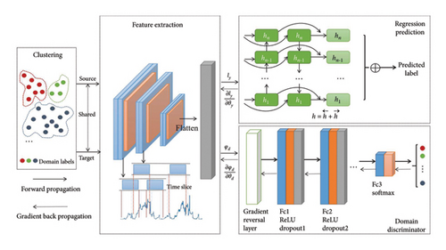
The subsequent section presents a description of the deep learning architecture-based air quality prediction framework, which incorporates transfer learning strategy. The composite model mainly consists of four modules: the clustering module divides different representation domains; the feature extraction module takes charge of acquiring local feature representations along with correlations of temporal data; the temporal prediction module learns long time-series data dependency; the domain classifier achieves source-to-target domain transfer of representations.

In the case of model transfer, the error upper limit was put forward by Ben-David et al. for target domain, which is determined by several key factors as follows:

$$ ()

where h = f°g, ε^t(h), and ε^s(h) refer severally to the losses on the target and source domains, respectively. $$ denotes the overall variation between the two distributions and λ_H represents the complexity of the forecasting hypothesis space H on both domains [44].

To allow transfer to unseen target domain from multisource ones, the above limit becomes:

$$ ()

where $$, the parameter $$ and $$, jointly decide the total divergence among domains [45]. The former parameter makes the multidomain representations approximate the target domain to the greatest extent, while the other one maximizes the differences between various source domains.

In order to enhance the generalizability of our model, it is necessary to ensure that the error upper bound after transfer is minimized. Firstly, we need to divide datasets from multiple stations into various source or target domains according to different strategies for subsequent representational transfer. Data are partitioned into separate domains through k-means clustering, thereby ensuring greatest diversity between domains and determining the lower limit of the model’s transfer capability. The principle of clustering can be formulated as shown below:

$$ ()

1D-CNN layers are used for feature extraction in our model. CNN allows effectively recognition of simple patterns in the data and their subsequent utilization for creating more sophisticated patterns in superior-level layers. CNN exhibits outstanding performance not only in image processing but also proven effective in mining time series data. A convolutional CNN comprises convolutional, activation, as well as pooling layers. In contrast to the traditional two-dimensional CNNs commonly used for image feature extraction, our proposal suggests utilizing multiple one-dimensional filters that are convolved across all time steps of time series data related to air quality. 1D-CNNs have a better performance on temporal features extraction. 1D-CNNs is extremely effective for obtaining feature representations of long time series data from shorter segments. For convolutional layer, its kernel function achieves data partitioning into time segments, and the position of the features in these segments are not highly correlated. The computing process of 1D-CNNs can be formulated as follows:

$$ ()

$$ ()

where $$ and $$ are the filters and bias, ReLU is the activation function. The nonlinear representation $$ is then fed into a flatten layer for conversion of high-level representation into a flattened format. 1D-CNNs have proven to be effective in analyzing audio signals and other signal data that are invariant in length periods, which are also preferably suited for time series analysis from sensors additionally.

Bi-LSTMs and bi-GRUs are applied for learning long temporal dependencies. LSTM maintains an internal state at each time step, which can selectively add or remove information using the input, forget and output gates [46]. Computing process of LSTM unit can be formulated as follows from equations (7) to (12).

$$ ()

$$ ()

$$ ()

$$ ()

$$ ()

$$ ()

where the input gate i_t quantifies the amount of information addition from the input and the prior hidden state, the output gate o_t judges if information from the cell state should be output to the hidden state; the forget gate f_t quantifies the amount of information eliminated from the cell state. LSTM can handle long sequences by allowing the cell state to be passed across multiple time steps without suffering from vanishing or exploding gradients efficaciously.

GRU resembles LSTM in that it regulates the information flow with gates as well [47]. But it merely has an update along with a reset gates. Its computing process is shown below:

$$ ()

$$ ()

$$ ()

$$ ()

where the update gate z_t quantities the extent by which the new hidden state is derived from the prior hidden state and how much is derived from the current input, while the reset gate r_t identifies the extent to which the prior hidden state should be forgotten. GRU is simpler than LSTM and has fewer indices, enabling its faster training and lower probability of overfitting. But its processing of ultra long time series data might be worse than LSTM. The bi-directional RNN achieves global information capture for time-series data, as well as training of two RNNs instead of one RNN on the input sequence. In the input sequence, the initial item is pristine, while the second item is a mirrored replica of the input sequence. This inclusion of additional context can greatly benefit the network, accelerating and enhancing its ability to tackle a wide range of learning problems effectively. So the final output is shown as follow:

$$ ()

where $$ denotes forward output and $$ represents backward output. Concatenation of the two yields the final output. This measure allows the model to learn from both past and future features presentation in time-series data. As a result, the forecast output is derived by considering the contextual information from both the past and future instances.

Fully connected layers are chosen as domain classifier for temporal distribution matching. For two different transfer strategies, they are set as binary classifiers or multiple classifiers respectively. In order to avoid segmented training and achieve better results in domain confrontation, a gradient reversal layer (GRL) is introduced, which serves as an identity transformation in the course of forward propagation. Contrastively, it automatically reverses the gradient direction during the back propagation. The relevant mathematical expression is shown as follows:

$$ ()

$$ ()

$$ ()

$$ ()

where I stands for an identity matrix, and λ_p represents a hyperparameter that dynamically changes with the iteration process. Let L denotes the length of minimum overall batches taking into account the target and source training data; j represent the current quantity of batches; k and n separately represent the current and overall quantities of iterations. The GRL primarily resides between the domain classifier and the feature extractor. As a result, in the course of backpropagation, there is an automatic reversal in gradient of the classifier-induced domain classification loss prior to propagating back to the extractor indices. This effectively leads to an adversarial loss computation, resembling that of GAN, but with simultaneous computation. Figure 1 displays the overall framework diagram of the model. Clearly, the framework comprises these four parts: the domain classifier, as well as each one module for clustering, features extraction and temporal forecasting.

4. Experimental Results and Analysis

In this section, we evaluate the performance of our model through experiments using an urban air quality dataset. Two strategies are employed for effective representation transfer. Three sets of comparative experiments are conducted to analyze and validate the prediction performance and effectiveness of our model. Firstly, our model is contrasted with traditional recurrent deep learning models and composite models that do not adopt transfer strategies. Secondly, we validate the effectiveness of introducing 1D-CNNs as feature extraction layers in our model. Finally, our model is subjected to performance validation on datasets from varying domains to assess whether the knowledge obtained from the transfer process has an auxiliary effect on the prediction of the original dataset. We choose the urban air quality dataset, which includes locational and meteorological data. It consists of six different components of data collected during the Urban Air project undertaken by the Microsoft Research Urban Computing Team. The data components are city data, district data, air quality data, weather prediction data, quality station data, and meteorological data [17]. The dataset covers a 1-year span, specifically from May 1, 2014, to April 30, 2015. Table 1 lists the dataset details. The hourly dataset is utilized to deduce detailed air quality for present and upcoming time periods. It is divided into two clusters based on city distributions: cluster A (19 cities near Beijing) and cluster B (24 cities near Guangzhou). The dataset contains a total of 2,891,393 hourly records from 437 air quality monitoring stations, with data items including various air indicators and geographical environmental indicators.

The dataset is divided into two segments: the training set (districts 1-42) and the testing set (district 43), ensuring different data distribution between sites. To facilitate the model’s learning of hidden relationships in temporal data, we map and concatenate data tables, filter useful attributes, and label each record according to different locations. Enumerate type data is mapped to the corresponding number tables. Labels are assigned based on two different strategies: DA and DG. For DA, Cluster A serves as the source domain, while cluster B is chosen as the target domain. For DG, each city is considered a separate domain. To enhance the model’s learning efficiency, we clean and complete the missing data, normalize all data, and replace missing data with means. For the missing number of location or district, we complete it with the largest number marked by the district. The processor and GPU used for conducting experiments are Intel Xeon (R) and GeForce RTX 3090. All the experiments are implemented in Python 3.8 along with the PyTorch 1.7 framework.

For the time series prediction module, we use bi-GRU and bi-LSTM as the baseline. The feature extraction module consists of three one-dimensional convolution layers model with dropout applied at each layer to improve model performance. For domain classifiers, a binary classification method (pattern) is employed for DA, while a multiclassification method (pattern) is utilized for DG based on the number of districts.

To achieve optimal prediction performance with the proposed transfer learning model, it is essential to determine the various hyperparameters following data preprocessing. To prevent overfitting, we use a dropout policy with a probability of 0.3. Default training parameters are set as follows: the batch size is 32, the epochs size is 100, the learning rate is 1e-3. For testing process, the batch size is 30 and the lookup size is 1. The activation function [tanh] is used in the RNN model including GRU and LSTM, while ReLU is the activation function for the conv1d layers. The Adam algorithm is applied as an optimizer. Both the proposed hybrid model and the models used for comparisons apply identical baseline modules. Three convolution layers are used for feature extraction of air quality time series data. The filter number and the kernel size in each convolution layer are different, which are set as (64, 5), (32, 3), (16, 1), respectively. The bi-directional time series prediction model has 3 layers, with a hidden size of 128 for each layer. In order to enhance training performance, normalization using the min-max function is employed to scale the data to the range of [0, 1]. Moreover, any missing values present in each column (attribute) are substituted with the respective column’s mean value.

To demonstrate the effectiveness of the two proposed transfer strategies, we utilize time series data from observation stations in different regions to train the models. The objective is to predict the air quality of the test district by leveraging the trained models. Various modules are combined for evaluating the forecasting performance, and further details are provided as follows. Module l: Convolutional layers for feature extraction. Module 2: Multilayers bidirectional recurrent network trained on data for regression prediction. The baselines chosen for comparison are GRU and LSTM. Different transfer strategies are utilized for comparison. Nontransfer: Train the models only using source domain data without domain shift. Strategy DA: Binary classifier for DA on hybrid networks that transfer knowledge from the source domain to the given target domain. Strategy DG: Multiple classifiers for DG on hybrid networks that transfer knowledge from multiple source domains to the unknown target domain.

As shown in Table 2, different model combinations yield varying prediction errors. Notably, models incorporating transfer learning strategies exhibit substantial performance improvements over nontransfer models. In particular, DA and DG significantly reduce RMSE and MAE, demonstrating their effectiveness in mitigating distribution shifts between training and test sets. Among these strategies, DA consistently achieves the best performance, with the DA-conv-LSTM model achieving the lowest RMSE (2.8610) and MAE (30.2536). This highlights its superior ability to extract transferable knowledge and adapt to unseen data distributions. Additionally, models utilizing LSTM outperform their GRU counterparts, further underscoring the effectiveness of LSTM in capturing long-term dependencies in air quality forecasting.

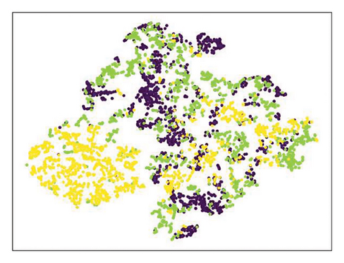
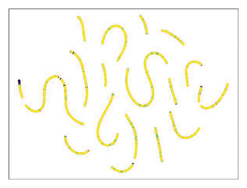
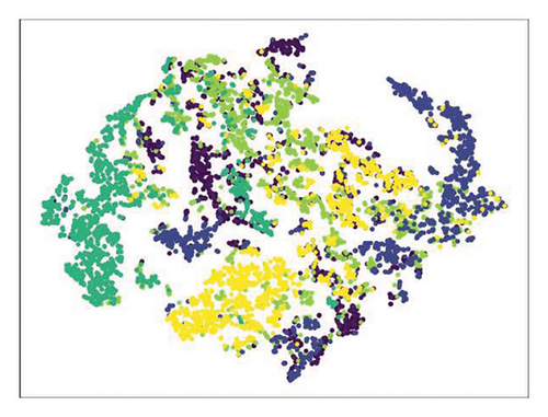
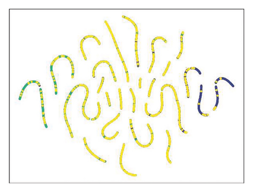
T-distributed stochastic neighbor embedding (T-SNE) is extensively employed to transform high-dimensional original data into a two-dimensional space for better visualization of data distribution [35]. Figures 2 and 3 show the scatter distribution shift of the original data inherent representation in two transfer strategies with T-SNE. For the DA strategy, we select station no. 101 in the source domain, station no. 14904 in the target domain, and station no. 37202 in the test set. It can be observed from the figure that the former one is separated, points of different colors are distributed in different positions. When using the transfer strategy for prediction, points are mixed indicating that there exists a definite domain shift between the source and target domain. For the DG strategy, we select any four source domain stations no. 101 no. 1718 no. 3502 no. 14904 and test set station no. 37202, respectively. It can be seen that it is consistent with the above condition. The primary reason for this is the significant divergence in data distribution across different districts, attributed to their distinct geographical conditions and climates. Consequently, the applicability of the model is limited to specific data, implying that a model trained in one domain typically exhibits poor performance in diverse domains.

Moreover, rather than employing the feature extractor, we directly counter the hidden layer output generated by the recurrent neural network. It can be observed from Table 3 that conducting adversarial transfer on hidden layers directly does not significantly reduce the values of RMSE and MAE, indicating that operating on hidden layers directly is not an effective domain matching strategy. The convolutional layers only learn representations through a fixed size time window (kernel size). Still, the number of parameters in the hidden layer on the time scale is much larger. Conducting adversarial transfer on these hidden layers runs the risk of sacrificing critical internal representation information, consequently escalating the computational complexity of the models.

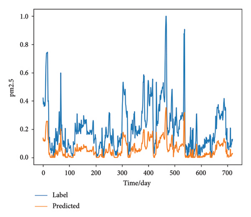
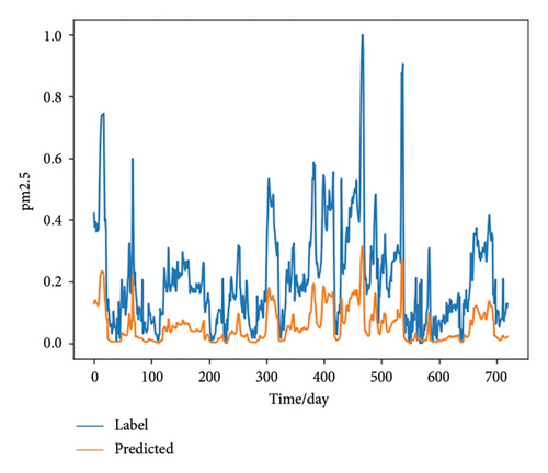
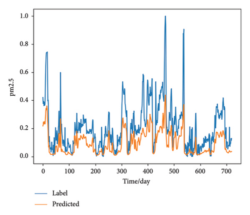
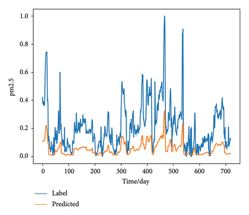
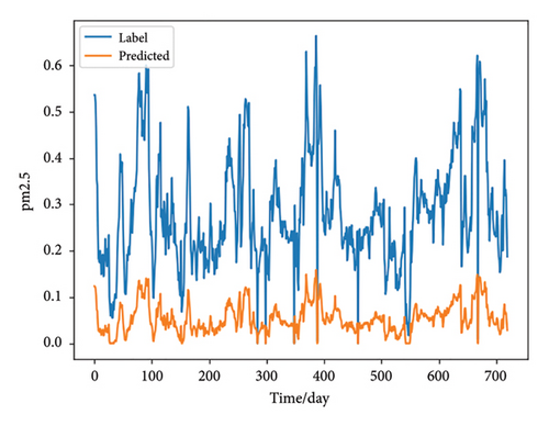
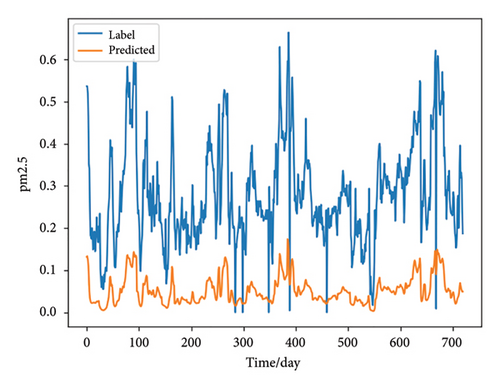
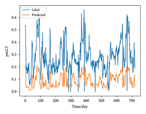
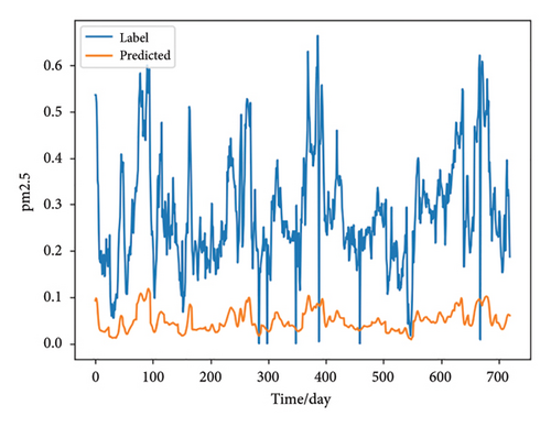
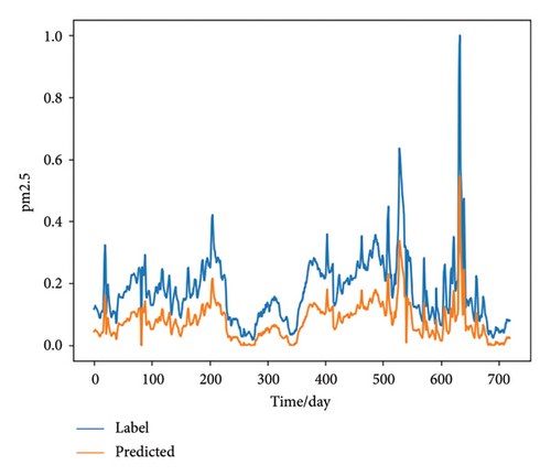
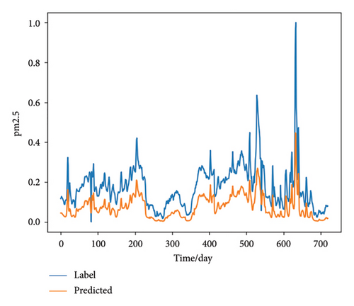
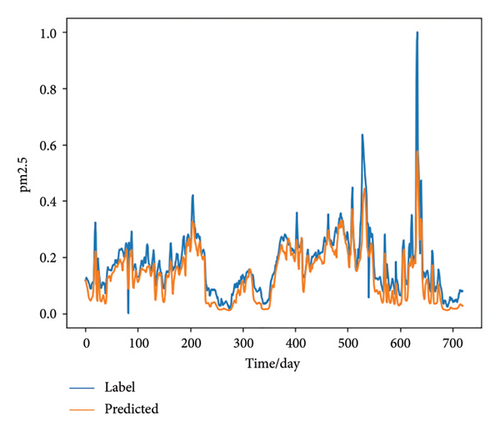
We predict the air quality of three stations in different domains during 2014-5-1 to 2014-6-1, station no.101 in the source domain, station no.14904 in the target domain and station no.37202 in the test domain, respectively. The concentration value of PM_2.5 is used as an indicator to display its changes in the next month. The lookup size is 24∗30, representing per hour for 1 month. Table 4 presents the performance evaluation metrics of various models for three stations. It is evident that the proposed hybrid model (da-conv-LSTM) exhibits superior performance in comparison to the other models. It indicates that the transfer model not only has better predictive performance on the original data but also exhibits good generalization ability.

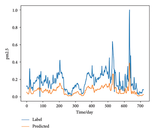
Figures 4, 5, and 6 further illustrate the comparisons between predicted labels and actual labels. The orange line represents the predicted value, while the blue line represents the actual value. The order of the images corresponds to the order of the models in Table 4, represented by the numbers (a)–(d) separately. It can be observed from Figures 4(b), 5(b), and 6(b) that the convolutional layer does not significantly impact the efficiency of the original model, but it can extract features faster and improve the performance of domain classifier. However, the results obtained from the DG strategy are not very impressive. Figures 4(d), 5(d), and 6(d) indicate that the representations learned by the model are too average in this case. For the source station, the error of the DA strategy is lower as seen in Figure 4(c). The predicted labels are very close to the actual labels indicating that the model has not lost the ability to predict the original data after transfer, and the transferred knowledge becomes a better auxiliary factor in improving accuracy. Similarly, for the target station, the same situation is noticeable in Figure 5(c). Despite significant differences in distribution from the source domain, the model exhibits certain predictive ability for target domains. For the test station, the DA-based hybrid model achieved excellent results in Figure 6(c). This demonstrates that the model possesses strong generalization capabilities and can make accurate predictions for data from unknown districts after directed transfer.

5. Conclusion

In this paper, we proposed a novel hybrid model with adversarial transfer methods for air quality forecasting in various stations. The goal was to eliminate domain differences and enhance the model’s generalization. Two kinds of transfer strategies were adopted based on the clustering results to address different transfer conditions. 1D-CNN layers were used to extract temporal features across different stations from time segments. Bi-LSTMs and bi-GRUs were applied for multivariate time series data predictions. Domain classifiers were applied to automatically reduce domain distribution discrepancies through adversarial transfer learning. The model trained with data from source stations can be directly used to assist in the prediction of the target stations. The efficacy of the proposed adversarial transfer based hybrid models was substantiated by experiments. The proposed model not only exhibited superior performance on an unseen target domain but also performed well on the original source domains. Nevertheless, there are several aspects that can be further improved and explored. One limitation is the potential for negative transfer, which can occur when irrelevant source domains introduce detrimental knowledge into the model. The model’s reliance on DG may lead to overly generalized representations, possibly due to limitations in GAN-based methods. Additionally, the model’s dependence on a sufficient number of source domains presents a challenge. If the available source domains are limited or highly biased, it could reduce the model’s ability to effectively generalize to the target domain. In future work, adversarial loss functions could be further refined to penalize harmful source domain information. Furthermore, reducing the reliance on large-scale labeled datasets by utilizing few-shot learning or self-supervised approaches for improved DA would be essential.

Ethics Statement

The authors have nothing to report.

Consent

The authors have nothing to report.

Disclosure

A preprint has previously been published [48].

Conflicts of Interest

The authors declare no conflicts of interest.

Author Contributions

Yanqi Hao: writing – original draft, writing – review and editing, validation, software, and methodology. Chuan Luo: methodology, conceptualization, writing – original draft, and writing – review and editing. Tianrui Li: formal analysis and writing – review and editing. Junbo Zhang: data curation and validation. Hongmei Chen: methodology, conceptualization, and writing – review and editing.

Funding

The current work was supported by the National Natural Science Foundation of China (Nos. 62476182, 62376230).