CSI Acquisition in Internet of Vehicle Network: Federated Edge Learning With Model Pruning and Vector Quantization
Abstract
The conventional machine learning (ML)–based channel state information (CSI) acquisition has overlooked the potential privacy disclosure and estimation overhead problem caused by transmitting pilot datasets during the estimation stage. In this paper, we propose federated edge learning for CSI acquisition to protect the data privacy in the Internet of vehicle network with massive antenna array. To reduce the channel estimation overhead, the joint model pruning and vector quantization algorithm for network gradient parameters is presented to reduce the amount of exchange information between the centralized server and devices. This scheme allows for local fine-tuning to adapt the global model to the channel characteristics of each device. In addition, we also provide theoretical guarantees of convergence and quantization error bound in closed form, respectively. Simulation results demonstrate that the proposed FL-based CSI acquisition with model pruning and vector quantization scheme can efficiently improve the performance of channel estimation while reducing the communication overhead.
1. Introduction
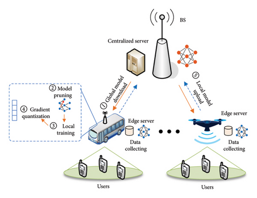
With the rapid development of Internet of things (IoT) and autonomous driving technology, vehicles and unmanned aerial vehicles (UAVs) have become more intelligent and IoT devices will generate a large amount of data, where those data need powerful communication and computer resource to realize the intelligent in-vehicle applications [1, 2]. Additionally, pushing the part of signal processing operation into the edge of networks is a powerful technique to reduce the transmission latency and communication overhead [3–5]. Nevertheless, the computing ability of vehicles or UAV is generally limited, due to the size of the device and power supply [6]. In this case, jointly using the centralized server at the roadside base station (BS) and edge server at the vehicles can efficiently leverage computing and communication resource. In order to make full use of the centralized and edge resource, it is necessary to exchange the information between the centralized server and edge servers. Especially in the context of the massive or extremely large-scale multiple-input multiple-output communication system, BSs are usually equipped with a large number of antennas [7–9]. Therefore, the accurate channel state information (CSI) acquisition becomes important. In current communication systems, the BS is usually equipped with massive or extremely large-scale antenna array, which leads to a large number of communication overhead [10]. It is well known that there exists two types of CSI acquisition mode in the current Internet of vehicle (IoV) communication systems, which are, respectively, called as pilot signaling–based channel estimation and beam training approaches [11, 12].
For the channel estimation with pilot signaling, it will generate lots of estimation overhead in the massive and extremely large-scale antenna array. To address the issue, the works on pilot-based channel estimation algorithm have been developed by utilizing the channel sparsity in angular or polar domain in the past few years, where the compressed sensing theory was exploited to reduce the pilot overhead for the massive or extremal large-scale antenna systems [13, 14]. Unfortunately, channel estimation with compress sensing method has to design the pilot matrix for satisfying the restricted isometry property [15, 16], which leads to the pilots randomization and makes the performance of channel estimation degradation. Alternately, the implicit CSI acquisition with beam training approaches has been proposed for massive frequency division multiplexing communication systems [17, 18].
Recently, machine learning (ML), such as reinforcement learning and graph neural network, has been introduced to uncover the nonlinear relationships in data/signals with lower computational complexity and achieve better performance for parameter inference and be tolerant against the imperfections in the data, which also has been applied into the channel estimation in wireless communication systems [19, 20]. They developed the conditional generative adversarial network framework to uplink-to-downlink mapping of both the CSI and channel covariance matrix, which can efficiently reduce the number of datasets. On the other hand, in the scenarios with some data privacy and sensitive security, e.g., IoV, railway, and bank, the conventional centralized learning algorithms are no longer applicable. Federated learning (FL), acting as a promising distributed ML methodology, was proposed to solve the information island phenomenon, which is able to alleviate privacy risks and the communication overhead required for uploading a large number of user data [21–23]. Therefore, the authors in [24] proposed the FL-based channel estimation algorithm to realize the goal of the global optimal estimation performance by exchanging between the centralize server and distributed server without collecting the original data. Different from the conventional CSI feedback or limited feedback strategies, an interacting federated and transfer learning framework for downlink CSI prediction was presented to solve the isolated data silos and online adaptation problem of CSI acquisition [25].
However, due to the unreliable wireless channel and limited wireless resource in the IoV networks, it is essential to develop effective communication and learning framework to improve the ultimate performance of wireless FL. In order to speed up learning rate and deal with high communication overhead of ML algorithm, several edge learning frameworks, such as federated edge learning, enable devices to compute local stochastic gradients, and transmit them to an edge server for aggregation and updating of a global learning model [26]. Since typical stochastic gradients in learning networks are of high dimensionality, transmission of the gradients parameters over communication networks can result in extensive overhead and a bottleneck for fast edge learning. To tackle this challenge, numerous schemes have been developed to reduce the communication overhead, where gradient compression is a common compression strategy. Specifically, the authors in [27, 28] proposed the scalar quantization scheme with “Quantized SGD” (QSGD) and “signSGD” and divided each dimension into several levels into compressing stochastic gradients so as to reduce the number of exchange parameters. Further, the authors in [29, 30] initially tried to explore vector quantization schemes to reduce the amount of communication symbol, where the edge devices communicate with the codeword index to the edge server rather than conveying the quantized version. Moreover, the adaptive period control schemes for the FL algorithm were presented to adjust the communication period so as to speed up the training while ensuring that the training loss is always minimized [31, 32].
Another aspect is to use the model compression technique to reduce the learning latency for local parameter calculation. To allow the different devices to participate in the model training with different model sizes, an ensemble distillation method for model aggregation was proposed in [33]. Based on the ensemble distillation method, network pruning has been adopted for FL to reduce the local model size [34]. Furthermore, the authors in [35] have proposed the adaptive pruning scheme to pruning the local model parameters by exploiting the similarity between the local model and global model, which can accelerate the convergence and reduce the updating overhead. While, the existing wireless FL investigated the homogeneous model settings where the devices train identical local models and the scale of the global model is restricted by the device with the lowest capability. To overcome the problem, an adaptive model pruning at the edge server by pruning the local model was proposed to adapt their heterogeneous computation capabilities [36]. In [37], the authors have developed the concept of the best sparsification levels to perform the model quantization operation. This approach is able to achieve the goal of minimizing the total energy while reducing the time consumption. Due to the gradients being redundant, the joint model pruning and scalar quantization was developed to reap the benefits of deep neural networks (DNNs) while satisfying the capability of resource-constrained devices [38]. Furthermore, it is noted that the device friendly and communication-efficient FL algorithm with model pruning and quantization can reduce storage, communication, and computation requirements, accelerating the training process in the IoT network [38].
- •
First of all, we propose an FL-based CSI acquisition framework for IoV network with massive antenna array, where the developed offline radio map scheme with FL framework can reconstruct the CSI of each user by collecting the channel feature information at the edge servers. The proposed FL framework provides decentralized learning network, which is suitable for more complex environments and large-scale scenarios compared to the traditional learning-based CSI acquisition techniques.
- •
Then, we propose the joint model pruning and vector quantization approach for the gradient parameters at the edge servers in the FL framework. The amount of exchange information between the centralized server and edge servers is reduced significantly by pruning and quantizing the gradient parameter of edge networks.
- •
Moreover, the impact of the network pruning and vector quantization on the learning performances is mathematically analyzed in closed form, where we analyze the mutual influence on the convergence rate of learning and quantization error bound, respectively.
- •
At last, we leverage the Wireless InSite software to construct the IoV network environment and illustrate the effectiveness of our proposed scheme by collecting datasets to train networks for CSI acquisition. The experiment results demonstrate that the proposed scheme can significantly reduce the model size and improve the communication cost while achieving high learning performance.
The rest of this paper is organized as follows. In Section 2, we introduce the system model with wireless FL. In Section 3, we propose CSI acquisition scheme via the FL framework with model pruning and vector quantization algorithm. In Section 4, the convergence rate and quantization error bound are analyzed, respectively. Then, experimental results are presented to verify the proposed algorithm in Section 5. Finally, Section 6 concludes this paper.
1.1. Notation
In this paper, the upper and lower case bold symbols denote matrices and vectors, respectively. We use (·)T, (·)T, (·)H, and |·| to denote the transpose, conjugate, Hermitian transpose, and absolute value, respectively. is the space of M × N complex-valued matrices and denotes the set. Symbols ⊗ and ⊙ stand for Kronecker and Hadamard product, respectively.
2. System Description
As shown in Figure 1, we consider the hierarchical cloud–edge–terminal communication network. This network consists of one BS and K edge servers (vehicle or UAV), where each server consists of Mk users and the total number of users is M, i.e., ∑Mk = M. In such system, we assume that the BS is equipped with UPA with N = NvNh antennas, where Nv and Nh denote the number of antennas along the vertical and horizontal direction, respectively. The edge servers and users are assumed to be equipped with single antenna. Generally, the acquisition of CSI is needed before each user communicates with BS via the wireless links. As the number of antenna becomes large in the future mobile communication systems, the CSI acquisition has to consume more pilot resource, which will reduce the spectrum efficiency of the communication systems. In this paper, we propose an offline radio map scheme with FL framework to reconstruct the channels of each user by collecting the channel feature information at the edge servers.
2.1. Cloud–Edge Communication Systems
2.2. Modified FL Model
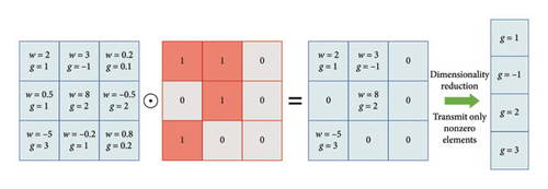
Different from the scalar quantization in the existing works [29], the codebook-based vector quantization can efficiently reduce the feedback overhead. Moreover, due to the sparsity of the model weight, we can attain the low-complexity quantization scheme by pruning model weight to alleviate the local computation overhead. The detailed model pruning and quantization scheme will be presented in the following section.
3. Model Pruning and Gradient Quantization Scheme
In practical wireless communication systems, the scale of the model parameter is huge and the aggregation of gradients would cause large communication signaling overhead and increase model training latency, due to the limited spatial–time–frequency resource. The conventional quantizing schemes may lead to great distortion under the limited bit budget, which will reduce the FL performance.
In this paper, the combination of model pruning and vector quantization scheme enables more efficient transmission of information under the limited bit budget within the FL framework. This motivates the compression of the model before transmission. Firstly, the network pruning can be applied before local training to reduce the model size. Secondly, the gradient vector quantization strategy is designed before uploading local model to further reduce the number of parameters that needs to be transmitted. Therefore, our goal is to design an encoding–decoding scheme, which reduces the communication signaling overhead and mitigates the effect of quantization errors on the ability of the centralized server so as to accurately recover the updated model.
3.1. Model Pruning
To improve the communication and computation efficiency for wireless FL, this paper develops a novel learning framework to adaptively generate submodels for edges to train. Moreover, to suppress the adverse effects of the local model in the learning performance, we leverage the gradients of the pruned model for interaction information.
3.2. Gradient Quantization
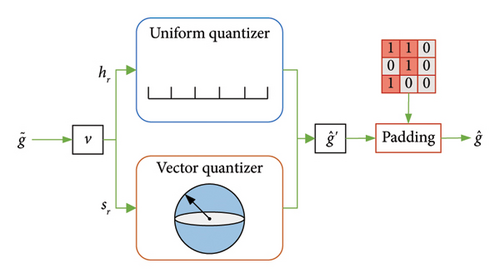
Unlike the conventional scalar quantization method, the advantage of vector quantization is the implementation complexity and model flexibility. Therefore, we propose the vector quantization to quantize the gradients evaluated over the pruned model to help reduce the uplink overhead in this paper.
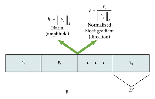
For high-dimension vector , we can partition this into multiple low-dimension vectors so as to reduce the quantization error. Specifically, we first partition high-dimension gradient vector into M segments with length D′, where each segment is quantized individually, i.e., . Therefore, vector vi can be deemed as the ith block gradient and is applied into zero padding if not exact division. Further, denote the normalized block gradient by si = vi/‖vi‖ and norm of block gradient by hi = ‖vi‖, respectively. Intuitively, si and hi represent the magnitude and direction of the normalized block gradient, respectively.
-
Algorithm 1: FL with model pruning and vector quantization.
- 1.
Initialize: Collect information of users at edge nodes and initialize global model.
- 2.
The global model broadcasts the utilized information to all edge nodes.
- 3.
For global iteration n = 1, …, N
- 4.
For each node k = 1, …, K
-
Compute weight value Ik,d, according to (8);
-
Compute gradient at the edge node based on dataset;
-
Obtain the reduce-dimension gradient ;
-
Feed back gradient to center node;
- 5.
End for
- 6.
The center node padding 0 elements into weight value
- 7.
Obtain global model via gradient cluster at center node
- 8.
The center node broadcasts information to all edge nodes
- 9.
End for
4. Performance Analysis
4.1. Quantization Error Bound
In order to represent the gradients , we utilize a finite number of bits inherently to induce the distortion and define the recovered vector as . Then, the moments of the quantization error satisfy the following lemmas.
Lemma 1. Let be a codebook designed by the line packing with resolution W and dimensionality D′. The average distortion [30] of normalized block gradient can be bounded as
Lemma 2. The distortion for quantizing the norm of block gradient vector h can be upper-bounded as
Theorem 1. The quantization error vector satisfies
Proof 1. Please refer to the proof in Appendix A.
It is observed from Theorem 1 that the quantization error decreases, as model pruning rate ρ increases. The reason is that it reduces the number of gradient blocks that needs to be quantified. Moreover, quantization error can also be decreased, as the codebook resolution W and the number of quantization intervals T grow. Further, as the length of the block D′ decreases, degrades accordingly in that pairwise distances between codewords enlarge but the number of gradient blocks will increase.
4.2. FL Convergence Analysis
Given a model pruning and quantization scheme for the stochastic gradient, we focus on the convergence of the learning algorithm, which is usually affected by the proposed model pruning and gradient quantization approach. Therefore, the convergence rate of the learning algorithm under will be theoretically investigated in this section.
Assumption 1 (L-smooth). The nonconvex loss function of the neural network F(·) is L-Lipschitz smooth, which can be written as
Assumption 2 (bounded stochastic gradients and model). The second moments of the stochastic gradients and weights are bounded, which can be guaranteed by l2-regularization and are also assumed in other works, such as [29, 30]. It can be expressed as
Note that l2 regularization effectively constrains the range of weight values by adding a penalty term to the loss function that is proportional to the sum of the squares of the weights, ensuring the stability of both stochastic gradients and weight boundaries. This aids the model in learning smoother and more stable solutions during the training process and results in better generalization performance on test data.
Assumption 3 (unbiased gradient). The locally estimated stochastic gradient is unbiased, which can be written as
Lemma 3. If Assumption 2 is valid, the model error of the kth device under the pruning ratio ρk satisfies
Theorem 2 (learning convergence rate). According to the model pruning and quantization method designed in this paper, on the premise of satisfying Assumptions 1–3, the learning convergence rate is expressed as
Proof 2. Please refer to the proof in Appendix B.
5. Simulation Results
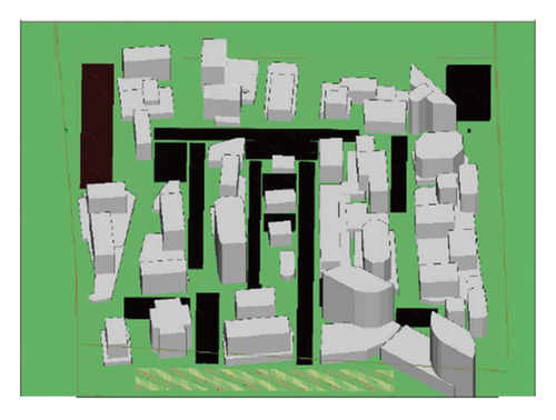
We conducted experiments on a simulated environment, where the number of edge server is set to K = 10 and one BS participates in the model training. The number of antennas at the BS is N = 256, where the number of antennas along the vertical and horizontal directions is set to Nv = 8 and Nh = 32, respectively. Each edge server collects 200 users’ channel characteristics as training samples and 100 users’ channel characteristics as testing samples. The users are evenly distributed in the coverage area of the BS. The information of the direct and reflection paths with the highest signal received power NL = 5 is stored at each sample. In this paper, Wireless InSite software [18] is used to collect datasets corresponding to channel acquisition models, where the ray tracing method is used to collect the effective path information of the users, as shown in Figure 5.
Furthermore, the proposed network architecture is a CNN with 9 layers. The first layer is the input layer, and {2, 4, 6} layers are the convolutional layers with NSF = 16, 32, 64 filters, respectively. Each filter employs a 3 × 3 kernel for 2-D spatial feature extraction. {3, 5, 7} layers are the activation layers. The eighth layer is fully connected layer and the last layer is output regression layer. The number of training iterations is 50, and the mini-batch size is 64. The Adam optimizer is leveraged to calculate the gradient of the loss function and update the parameters, and the learning rate is set to 0.01.
- 1.
Quantized stochastic gradient descent–based model pruning (QSGDMP) scheme: This scheme uploads QSGD quantization parameters with the model pruning strategy.
- 2.
TOPK: Each user only uploads the maximum K weight values.
- 3.
Vector quantized stochastic gradient descent (VQSGD) scheme: Each user uploads the parameters by exploiting only the vector quantization without model pruning.
- 4.
SGD: In this scheme, each user uploads the whole stochastic gradient descent information.
Figure 6 shows the curves of the MSE vs. the number of iterations for the different schemes. Except for the SGD scheme, we set the other four schemes to transmit the same number of bits for comparison. It is observed that the performance of SGD scheme is better than other schemes because the number of bits is sufficient can be transmitted, and SGD scheme requires a lot of communication overhead. The performance of the proposed scheme can be close to that of SGD and better than that of other schemes; the reason is that the center server shares and clusters the all user’s information. Moreover, the VQSGD algorithm is significantly worse than that of proposed algorithm, which means that improvements of learning performance is the introduction of model pruning.
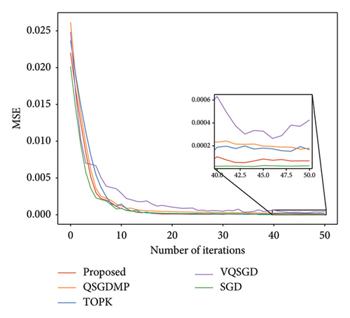
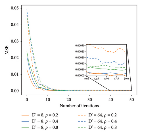
Figure 7 reports the curves of MSE vs. the number of iterations, where number of bits allocated to each block is fixed and the effects on block length D′ and pruning rate ρ are evaluated. It can be observed that as block length D′ increases, the performance of FL will be degraded. The reason is accordingly that the quantization error for the stochastic gradients enlarges. Furthermore, when the quantization error is relatively small, model pruning error plays a dominant role. In particular, the increase of the model pruning rate will lead to NMSE degradation. On the other hand, when the quantization error is large, quantization error plays a dominant role, and the increase of the model pruning rate will reduce the quantization error and the learning performance will be improved. Therefore, the model pruning rate needs to be set properly.
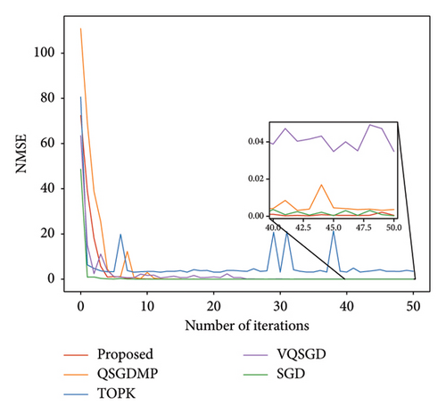
Furthermore, Figure 8 depicts the NMSE vs. the number of iterations for the different schemes. Compared to MSE in Figure 6, the gap of the proposed scheme of NMSE is obvious for the other schemes, since the NMSE is related to the number of test samples of each server k and MSE is related to the total number of test samples. Besides, the proposed scheme is more smooth for the NMSE performance, since the NMSE metric uses the number of test samples of each server applying the practical scenario.
6. Conclusion
In this paper, we proposed a FL framework for the CSI acquisition for IoV with massive antenna array. With the consideration of both the user privacy and wireless communication capacity limitation, we proposed the network pruning and vector quantization schemes applying into the wireless FL IoV system so as to reduce the model size. To evaluate the learning performance of the FL with network pruning and vector quantization, the convergence rate and quantization error bound have been mathematically analyzed, respectively. Finally, based on the Wireless InSite software, the effectiveness of the proposed algorithm has been demonstrated by the experimental results.
Conflicts of Interest
The authors declare no conflicts of interest.
Funding
This work was supported in part by the Natural Science Foundation of Henan (No. 252300421516), in part by the Scientific Research Team Plan of Zhengzhou University of Aeronautics (23ZHTD01005), in part by Key Projects for Joint Fund of Henan Province Science and Technology Research and Development Plan (225200810033), in part by Henan Center for Outstanding Overseas Scientists (GZS2022011), in part by Henan Province Collaborative Innovation Center of Aeronautics and Astronautics Electronic Information Technology, in part by the National Natural Science Foundation of China under grant no. 62371180, in part by the Anhui Provincial Natural Science Foundation under grant no. 2008085QF281, and in part by the Fundamental Research Funds for the Central Universities of China under grant no. JZ2024HGTG0311.
Acknowledgments
This work was supported in part by the Natural Science Foundation of Henan (No. 252300421516), in part by the Scientific Research Team Plan of Zhengzhou University of Aeronautics (23ZHTD01005), in part by Key Projects for Joint fund of Henan Province Science and Technology Research and Development Plan (225200810033), in part by Henan Center for Outstanding Overseas Scientists (GZS2022011), in part by Henan Province Collaborative Innovation Center of Aeronautics and Astronautics Electronic Information Technology, in part by the National Natural Science Foundation of China under grant no. 62371180, in part by the Anhui Provincial Natural Science Foundation under grant no. 2008085QF281, and in part by the Fundamental Research Funds for the Central Universities of China under grant no. JZ2024HGTG0311.
Appendix A: Proof of Theorem 1
Appendix B: Proof of Theorem 2
Open Research
Data Availability Statement
Research data are not shared.


