Fusion Network Model Based on Broad Learning System for Multidimensional Time-Series Forecasting
Abstract
Multidimensional time-series prediction is significant in various fields, such as human production and life, weather forecasting, and artificial intelligence. However, a single model can only focus on specific features of time-series data, making it unable to consider both linear and nonlinear components simultaneously. In this study, we propose a fusion network that combines the advantages of deep and broad networks for multidimensional time-series prediction tasks. The complex multidimensional time-series data are divided into nonlinear and time-series data. Restricted Boltzmann machine and mapping functions are used for feature learning and generating mapping nodes at the mapping layer. The echo state network and gate recurrent unit are applied in the enhancement layer. The proposed model has been validated on PM2.5 and wind turbine power datasets, proving superior performance in multistep prediction tasks compared to the baseline models.
1. Introduction
Time-series prediction refers to predicting future data based on historical patterns and trends in time-series data [1, 2]. Time-series prediction is widely utilized across multiple domains, such as the energy industry, where it can predict load demand, perfect power generation planning, and regulate electricity prices [3]. In the financial field, it can be used for stock market price prediction [4], foreign exchange market exchange rate fluctuations prediction, and interest rate trend prediction. Multivariate time series refers to multiple real numerical variables or descriptive attributes corresponding to the same moment. In multivariate time-series prediction tasks, the relationship between multiple data dimensions is no longer limited to the correlation between variables and time but also has certain connections between variables [5]. By predicting multivariate variables, we can better understand the relationships between variables, supply comprehensive data analysis and decision-making support, perfect resource planning, identify risks and take measures, and realize the modeling and control of complex systems and other needs. The application scenarios of multivariate time-series prediction include weather data prediction, industrial production decision-making, and the artificial intelligence field. With the accumulation of data and the development of technology, multivariate time-series prediction will continue to play a vital role in predicting the future and perfecting enhancing decision optimization.
Time-series forecasting models can be mainly categorized into traditional statistical regression, shallow networks, deep networks, and broad networks. With the increasing size and dimension of time-series data, traditional means of statistical analysis have been difficult to meet the demand [6]. Shallow networks have shifted from handling linear data in temporal forecasting tasks compared to traditional statistical regression models toward nonlinear data. Deep networks and broad networks build upon shallow networks by constructing network structures in depth and broad directions to adapt to the requirements of different time-series forecasting tasks [7]. Research has been conducted on prediction methods for multivariate time series. Mou et al. [8] proposed a time-domain enhancement-based long short-term memory model (T-LSTM). Based on the LSTM model, the intrinsic correlation between traffic flow and time series is fully utilized, which improves the accuracy of prediction. Multidimensional recurrent neural networks (MDRNN) is a variant based on improvements to recurrent neural networks (RNN) and is a neural network model used for processing multidimensional sequential data [9]. Unlike traditional RNNs, MDRNNs can effectively process input data with multiple dimensions. Conventional deep learning models such as LSTM and gated recurrent unit (GRU) have a particular ability to learn long-term dependencies in time-series data [10, 11]. They can alleviate issues like gradient vanishing or exploding. However, they still have limitations when handling multidimensional data with high-dimensional complex features. These limitations include long training and inference times due to high computational complexity, increased memory consumption caused by storing many intermediate states when dealing with long sequences, and weak modeling abilities for short-term dependency relationships. More flexible and powerful models are needed to capture the complexity of multidimensional time series.
Broad learning networks and their variants map and enhance multidimensional data to learn more time-series features, obtaining output weights through pseudoinverse fast solutions [12]. Philip Chen and Liu [13] proposed a broad learning system (BLS) that combines augmentation nodes with an input layer, making it possible to expand the network laterally by increasing the number of nodes in the hidden layer of the BLS. Owing to the absence of backpropagation and gradient descent, BLS typically exhibits faster training times than conventional deep learning models. Chen et al. [14] proposed a BLS-RVM algorithm combining BLS and random vector machine (RVM) regression to improve the prediction of the remaining lifetime of lithium-ion batteries. However, the performance of these methods is not yet satisfactory. Multivariate time series often show nonlinearity, temporal characteristics, and interdependencies among variables. First, existing prediction methods for multivariate time series often only consider the nonlinear relationships of the data and treat multiple variables at the same timestamp as inputs for prediction when constructing the network. Although this approach, to some extent, captures the correlations among different variables, it overlooks the temporal characteristics of the multivariate time series, where the relationships and trends between variables change over time. Besides, broad learning has a performance advantage over deep network learning due to its incremental learning approach, which addresses the issues of time-consuming training and high hardware requirements [15]. However, in practical applications, it is frequently observed that a solitary broad learning network may not yield the most optimal outcomes. Consequently, the integration of complementary methodologies or a synergistic ensemble of techniques can significantly enhance predictive accuracy [16]. Modifying the broad learning network is necessary considering the difficulties faced in multidimensional time-series prediction.
- 1.
To address these limitations, this study introduces a novel prediction model for multidimensional time-series data, which is grounded in the architecture of the broad learning network. A feature extraction method is proposed for multidimensional time-series data within the broad learning framework, and echo state networks and GRU are introduced into the learning process [17, 18]. This is important in improving the accuracy and efficiency of time-series prediction.
- 2.
Aiming at the problems that deep learning is susceptible to local optimum and gradient-related problems, the width learning system can make up for the shortcomings of deep learning to a certain extent, making it more efficient in dealing with new data and network node adjustment and providing a flexible and powerful width framework for multidimensional time-series prediction models.
- 3.
The incremental algorithm is used to optimize the network structure, adding nodes in the hidden layer to construct the network in the direction of “width,” without reconstructing the model, only need to modify and expand the original weights to get the new model parameters, and also be able to extract abstract and rich features.
The remainder of the paper is structured as follows. Section 2 reviews the current state of research in time-series forecasting, specifically focusing on multidimensional time-series forecasting. In Section 3, we provide a detailed description of the network structure and algorithm of the proposed Mix-BLS model. Section 4 presents a comprehensive experimental comparison and analysis of the proposed model against the control model across two distinct datasets. Finally, Section 5 summarizes the key findings of this study and suggests directions for future research.
2. Related Works
2.1. Time-Series Forecasting Methods
Time-series forecasting models can be divided into traditional statistical regression, shallow networks, deep networks, and broad networks. The traditional statistical regression techniques encompass models such as autoregressive model (AR) [19], moving average model (MA) and autoregressive moving average models (ARMA) [20, 21]. The autoregressive integral moving average model (ARIMA) [22–24] is an extension of the ARMA [25]. The AR is more suitable for stationary time series, while the ARIMA [26] is used for nonstationary time-series data. The model combines the AR, MA, and difference method [27]. The traditional statistical regression approach boasts a straightforward structure, underpinned by a rigorous theoretical derivation, endowing it with high interpretability. This characteristic renders it particularly effective for the analysis of online linear data and for the execution of short-term forecasting tasks, often yielding superior outcomes. Concurrently, traditional statistical regression techniques methods exhibit notable limitations. Their efficacy is contingent upon the judicious selection of model parameters and necessitates a high degree of data linearity. This reliance on linear assumptions complicates the accurate fitting of intricate nonlinear datasets. Therefore, for current time-series forecasting problems, the application scenarios of traditional statistical regression methods are relatively limited.
In response to the limitations of traditional statistical regression methods, a machine learning-based forecasting approach has been introduced, mainly including artificial neural networks and support vector machine (SVM), which belong to shallow networks. The artificial neural networks [28] are renowned for their robust learning capabilities. As a quintessential machine learning model, the backpropagation neural network is adept at modeling simple time-series data. SVM is proposed from the best classification surface in the case of linear separability [29]. The machine learning-based prediction model [30] benefits from a well-established theoretical foundation, a straightforward algorithmic structure, and inherent self-learning and adaptability capabilities, making it suitable for modeling nonlinear data. However, the current volume and high volatility of collected time-series data render these machine learning methods inadequate for effectively fitting nonlinear data tasks.
Currently, prediction models based on deep learning methods are widely used in time-series data prediction, mainly including RNNs, long short-term memory networks, and GRUs [31, 32]. The RNN [33] considers the current moment’s input and the earlier moment’s output information when constructed and has a good modeling ability for nonlinear time-series data. Confronted with extensive time-series datasets, RNNs are prone to encountering issues such as vanishing and exploding gradients, thus extending the long short-term memory network [34]. LSTM is equipped with a series of gating mechanisms that effectively integrate short-term and long-term memory, thereby significantly addressing the issue of vanishing gradients. GRU has been introduced to further refine the parameters of the long short-term memory architecture. The architecture of this model incorporates only update and reset gates, which simplifies the computational process and results in a faster computation speed compared to the LSTM network. Deep learning-based prediction models [35] are adept at uncovering the latent features within data, demonstrating a potent capacity for discerning nonlinear relationships. Despite its powerful learning capabilities, deep learning methods require substantial data to achieve optimal performance. Although the deep learning method has a robust learning ability, this learning ability requires a high amount of data. Insufficient data provision typically leads to suboptimal prediction accuracy. Moreover, the presence of noise within the data can impede the learning process of neural networks. The training converges and even leads to overfitting.
In response to challenges encountered in deep learning, the development of broad learning has emerged as an alternative to traditional deep networks. Unlike the conventional approach of extending network depth, broad learning chooses to complete feature transfer by adding neural nodes laterally to solve the problem [36]. Random vector functional link network (RVFL) [37, 38] is a type of planar neural network where the weights between the input data and the hidden layer are randomly initialized to reduce training time and computational demands. RVFL effectively integrates input data with nonlinear features generated during training and establishes a direct connection to the output layer. Compared with the complex deep neural network, the structure of the random vector function link neural network is simple. Compared with the complex neural network, fewer parameters need to be updated, the weight calculation is convenient, and it also has strong generalization ability. However, random vector function linking neural networks face certain limitations. As big data emerge, directly linking input data to the output layer can hinder the system’s maintainability and accessibility.
The existing methods have their limitations in the time-series data prediction field. Traditional RNNs are often plagued by limitations such as susceptibility to local optima and challenges in maintaining stability. Current methodologies typically involve a singular structure with limited generalization capabilities. Concurrently, the field of deep learning is encountering its own set of developmental challenges. The predictive capabilities of models are significantly constrained by dataset-related factors, including data volume and the degree of nonlinearity, which can critically impact both computational efficiency and model accuracy. Furthermore, these models are typically vulnerable to noise interference, which can diminish accuracy and, in severe cases, lead to overfitting.
2.2. Multidimensional Time-Series Forecasting Methods
Multivariate time-series data inherently have strong complexity, nonlinearity, and temporal characteristics. Multivariate time series constantly change, and their data size is generally large. The dimensions of multivariate time series are highly correlated, and it is essential to consider the situation of each dimension comprehensively to obtain more meaningful results. Separating the dimensions can lead to the loss of valuable information. Wang et al. [39] adopted a new template matching method to adaptively extract specific periodic features and reassemble one-dimensional time series into natural structured data of multiple sequences. To reassemble one-dimensional time series into naturally structured multidimensional data, added processing and operations are needed for the original data. This reassembling process may introduce added noise or result in information loss, thereby affecting the accuracy of prediction results. Using a multivariate LSTM network to handle expanded sequences may increase the complexity of the network. Complex network structures can lead to increased time costs for training and inference, as well as higher demands for computational resources.
The structure of multivariate time series is extremely complex. On the one hand, multivariate time series originate from various application domains in real life. The sampling methods and measurement standards differ between different sequences and even among dimensions of the same sequence. Additionally, multivariate time series show frequent fluctuations, noise interference, and nonstationarity. Fan et al. [40] proposed an integrated model combining ARIMA and LSTM. The ARIMA model is used to filter the linear trend in the production time-series data and pass the residual values to the LSTM model. However, this manual approach of handling linear trends may not be flexible or correct enough. For complex or nonlinear trends, the ARIMA model may not effectively capture them, thus affecting the overall predictive ability of the model. Karasu et al. [41] proposed a new prediction model based on support vector regression (SVR) and wrapper-based feature selection method. This method involves multiple parameters such as SMA, EMA, KAMA, etc., which require more computational resources and time to adjust and may increase the risk of overfitting or underfitting. Additionally, multiple-objective optimization techniques are needed to handle the feature selection problem, leading to relatively longer training time. When dealing with large-scale data, slow computation speed may also be met.
Traditional statistical regression methods have complete theoretical derivation processes and procedural modeling steps, making them easy to understand. However, they heavily rely on the judicious selection of parameter models and necessitate a high degree of data linearity, which can render the fitting of intricate nonlinear datasets a formidable task. Shallow networks have a certain degree of self-learning and adaptive capability. However, in the era of big data, shallow networks show limited nonlinear expressive power and cannot capture long-term dependencies in time-series data. Existing time-series networks, to some extent, can capture the correlations between different variables but overlook the temporal nature of multivariate time series. This means that the relationships and trends between variables can change over time. Conventional one-dimensional time-series models have excellent capability to learn temporal dependencies. However, they cannot capture relationships among multiple correlated variables or consider the influence of other potential variables on the current variable. This limitation may result in less correct and complete predictions. But multivariate time-series models simultaneously consider the nonlinearity among multiple variables and the temporal nature of the data. This helps reveal the correlation patterns and influencing factors among different variables. Compared to traditional one-dimensional time-series models that only consider a single variable, multivariate time-series models need to consider the influence of other potential variables on the current variable.
With increased data dimensions, model training and prediction complexity also increase, requiring higher computational capabilities. Therefore, more computational resources and storage space are needed. Although deep neural networks have powerful learning capabilities, they need much data for best performance. Insufficient data can lead to subpar prediction accuracy [42]. Additionally, the presence of noise in the data can affect the learning process of deep neural networks, resulting in training convergence issues or even overfitting. Existing deep neural network time-series models are designed with complex structures, employing sophisticated optimization algorithms and iterative processes to construct and adjust the network [43]. They also involve numerous hyperparameters and require ample training data to achieve high accuracy. Compared to deep neural network models, which often consume a significant amount of time during training, the advantage of incremental learning in broad networks can simplify parameter adjustment and reconstruction processes, significantly saving computational resources and showing promising applications. A single model can only focus on specific features of time-series data, inevitably losing some information when predicting time-series data. Therefore, exploring the combination of models to carry out prediction tasks has become a hot research topic. Wu et al. [44] proposed a broad fuzzy cognitive map system (BFCMS) to address the multidimensional time-series classification problem. However, there was no discussion or solution on how to optimize the BFCMS by removing some redundant nodes to forget some toxic data. Xiong et al. [45] proposed a dynamic adaptive graph convolutional transformer integrated with a broad learning system (DAGCT-BLS) to enhance the prediction accuracy of multidimensional chaotic time series. Due to the integration of multiple deep learning techniques, this model may require substantial computational resources. Su et al. [46] proposed a multihead attentional broad learning system (Multi-Attn BLS) that integrates BLS with a multihead attentional mechanism to effectively extract key spatiotemporal features from chaotic time series, resulting in high prediction performance. However, the effectiveness of this method has not been validated for multistep or long-term predictions. Zhu et al. [47] proposed a multidimensional information fusion and BLS (MIFBLS)-based model for identifying pipeline radiation threat conditions to improve the security of energy pipelines. However, the experimental validation was primarily executed using datasets derived from natural gas pipelines, and the model’s capacity to generalize was not further evaluated across a broader spectrum of pipeline types or under varied environmental conditions. Yuan et al. [48] proposed a joint spatiotemporal feature learning framework for multivariate TSP, consisting of a mixture of multiple sparse autoencoders (SAE) and multiple higher-order fuzzy C-means (HFCM) modules to model the spatiotemporal dynamics of these feature sequences. However, STFCM has many parameters, which makes it difficult to select the appropriate combination of these parameters through grid search. Therefore, more correct predictions can be achieved only by comprehensively considering the nonlinearity and temporal nature of multivariate time series, especially when multiple variables show complex interdependencies and patterns over time.
3. Fusion Network Model Based on BLS
3.1. Structure Design of Fusion Network
Multidimensional time-series data are inherently complex, exhibiting nonlinearity, temporal dynamics, frequent fluctuations, noise interference, and nonstationarity, which attributes present substantial challenges for forecasting models. Utilizing a BLS framework for multidimensional time-series forecasting can streamline the parameter tuning and model reconstruction process, thereby reducing training duration and enhancing predictive accuracy. Traditional time-series models and deep learning networks can effectively handle multidimensional time-series data’s nonlinear and temporal components. Therefore, fusing deep networks introduces a novel approach for predicting multifaceted time-series data in the broad system framework, simultaneously considering the nonlinear and temporal aspects of time-series feature information. The network structure is illustrated in Figure 1.
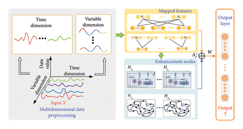
The main focus of the proposed fusion network in this article is to address the nonlinear and temporal issues in multidimensional time-series prediction simultaneously. The multidimensional time-series data are classified into temporal and nonlinear features, with solid-colored lines indicating temporal features in the data, that is, data for each variable over a range of time, and miscellaneous-colored lines indicating nonlinear features, that is, data for different variables at the same point in time. The network is structured into an input layer, mapping layer, enhancement layer, and output layer.
3.1.1. Input Layer
The input layer performs a first feature transformation on the multidimensional time-series data. Assuming there are f groups of mapping nodes and e groups of enhancement nodes, the original multidimensional time series X is divided into nonlinear data and temporal data , which are then inputted to the mapping layer. Nonlinear data XN refer to the data from different sequences in the multidimensional time series, where variables show certain correlations. Temporal data XT, on the other hand, represent attribute data corresponding to consecutive moments in time, where variables have correlations with time. When inputting temporal data, the label data from previous moments and the current moment are also included as feature inputs to the mapping layer of the network.
3.1.2. Mapping Layer
3.1.3. Enhancement Layer
The echo state network reservoir pool consists of numerous sparsely connected neurons. By adjusting the characteristics of the reservoir pool weights, it can learn the nonlinear mapping of input data, thereby extracting complex nonlinear features and generating enhancement nodes. Additionally, the reservoir pool possesses short-term memory capabilities. On the other hand, GRU is capable of learning the long-term and short-term dependencies in temporal data, preserving important feature information from the sequential mapping data to generate enhancement nodes while mitigating the impact of the vanishing gradient problem.
3.1.4. Output Layer
3.2. Learning Method of Fusion Network
Based on the design of the fusion network structure, research is conducted on the training and learning methods of the network.
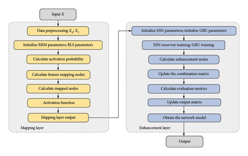
Algorithm 1 details the construction and learning processes of the fusion network. Additionally, the training process of this network is illustrated in Figure 2.
-
Algorithm 1: Training process of fusion network.
-
Input: training samples X;
-
Output:W
-
Input data preprocessing: nonlinear data XN; time-series data XT
-
for 1 ≤ k ≤ f; 1 ≤ l ≤ e; 1 ≤ i ≤ f do
-
Initialization v1 = X0, e, ε, T. Random Wvh, ak, bl, (Wi, βi).
-
Calculate ;
-
Update Wvh, ak, bl, (Wi, βi);
-
Calculate ZN = Φi(XNWvh + ai); ZT = Φi(XTWi + βi)
-
end
-
Set the feature mapping group ZT+N = [Zt1, Zt2, …, Ztf|Zn1, Zn2, …, Znf];
-
for 1 ≤ j ≤ e do
-
Initialization N, rho, cr, lr, α; Random , Win, Wz, Wr;
-
Calculate ;
-
Calculate ;
-
end
-
Set the enhancement nodes group ;
-
Set the hidden layer output matrix ;
-
Calculate
-
Set and calculate with equation (11);
-
The incremental algorithm:
-
Random , Win, Wz, Wr;
-
Calculate ;
-
Set ;
-
e = e + 1;
-
end
-
set W = W′
Multidimensional time series continuously change over time, and they typically have a large data size. Each time point in a multidimensional time series corresponds to multiple variables, resulting in a high-dimensional structure. In contrast to deep learning models, which rely on iterative processes for weight updates and are susceptible to challenges such as local optima and gradient-related issues, the broad learning framework circumvents these pitfalls. Additionally, the broad learning framework extends the network in a broad direction by increasing fusion nodes and feature nodes, which helps alleviate the problem of long training time caused by a deep network architecture. For predicting multidimensional time series, the fusion network adopts a BLS framework that incorporates traditional time-series models and deep learning network models to handle nonlinear and temporal data, respectively. This method heightens the model’s capacity for nonlinear representation and its efficacy in capturing prolonged dependencies within time-series data, leveraging the benefits of both broad learning and deep learning methodologies.
4. Experiment and Result
To validate the effectiveness of the proposed method, this study conducted experiments using two datasets. The experiments were executed on a 64 -bit Windows 10 system equipped with an AMD Ryzen 7 4800H processor and 16 GB of RAM. The implementation was carried out using the Python programming language, with PyCharm serving as the development environment.
4.1. Datasets
The datasets employed in this study are the Fangshan air quality data and wind turbine power data, both of which were sourced from real-world environments.
4.1.1. Fangshan Air Quality Dataset
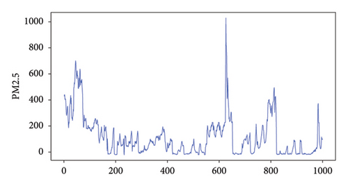
A city’s air quality directly affects the residents’ well-being and health. Governing atmospheric pollution, improving air quality, strengthening scientific prevention and control of air pollution, and promoting green development are the current trends in social development. This study uses the Fangshan air quality dataset from Beijing, which includes seven variables: CO, NO2, O3, SO2, PM10, AQI, and PM2.5. The Fangshan air quality datasets are collected from real environments, which are fully natural environments and are highly realistic and representative. The data are collected at hourly intervals. PM2.5 concentration is an essential factor influencing the number of days with good air quality, making its prediction highly significant. The proposed model’s predictive performance is evaluated by forecasting the changes in PM2.5 concentration. The original PM2.5 data are shown in Figure 3. The first 18,000 data points are used as the training set, while the last 6000 data points are used as the testing set. The input includes the previous six variables, and the output is the next variable, with a moving step size of three, for example, using multidimensional variable data from time (t − 3) to (t − 1) to predict the PM2.5 concentration data from time t to (t + 3), and so on for further predictions.
4.1.2. Wind Turbine Power Dataset
With the global urgency to reduce carbon emissions and achieve carbon neutrality, wind power plays a significant role as a low-carbon energy source in conducting these goals. Wind power forecasting aids power system operators in accurately understanding future wind power generation, supplying crucial information for power system operation and scheduling. This, in turn, eases better planning and optimization of energy dispatch, avoiding unnecessary energy waste. Wind power forecasting promotes and adopts clean energy, reaching low-carbon environmental objectives and establishing a sustainable future energy system.
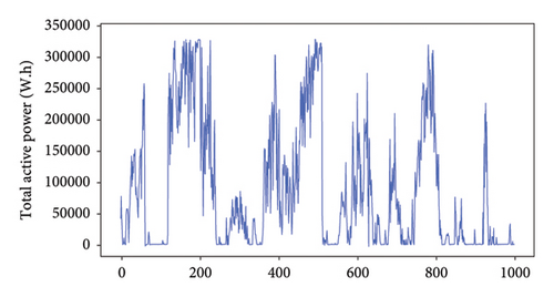
This experiment uses the Wind Farm dataset from the EDP Open Data portal, specifically the power dataset of wind turbine T11 in 2016, to validate the proposed model’s performance. Given that the dataset is influenced by human factors, accounting for these elements can enhance the model’s ability to discern underlying patterns and features, thereby improving its predictive accuracy and robustness. And it is publicly available, which increases the reproducibility and comparability of the results, and facilitates the validation and expansion of this research by other researchers. The dataset consists of six variables: average wind speed, average pressure, average humidity, average wind speed within a given time interval, average wind relative direction, and total active power. The measurements are taken at a 30-min interval. Figure 4 presents the raw total active power data, revealing significant fluctuations in wind turbine power. The first 15,000 data points are used as the training set, while the remaining 2475 data points serve as the testing set. The prediction task involves using the first five variables to predict the next variable with a moving step size of three. For instance, predicting the raw total active power data from time (t − 3) to (t − 1) using multidimensional variable data and continuing this pattern for future predictions.
4.2. Experimental Results
Symmetric mean absolute percentage error (SMAPE) measures the average absolute percentage deviation between predicted and actual values. A smaller SMAPE indicates higher prediction accuracy. Mean absolute percentage error (MAPE) quantifies the average absolute percentage deviation of individual data points from their arithmetic mean, providing a measure of forecasting accuracy. A lower MAPE indicates better predictive ability of the model. Relative squared error (RSE) is the ratio of the mean-squared error (MSE) to the average variance between predicted and actual values. A smaller RSE indicates a better predictive ability of the model. Relative root-mean-square error (RRMSE) is a statistical metric used to evaluate the predictive accuracy of a model. A smaller RRMSE value signifies higher prediction accuracy of the model. The correlation coefficient, denoted as R, quantifies the linear association between predicted and actual values. An R-value nearing 1 signifies a robust linear relationship.
In this experiment, eight models were evaluated on two datasets separately, using multistep prediction with a moving step size of 3. For the Fangshan dataset, the first six variables were used to predict the last variable. The training set consisted of the first 18,000 data points, while the remaining 6000 data points were gave as the test set. The original data are shown in Figure 3. As for the wind turbine power dataset, the first five variables were used to predict the last variable. The training set included the first 15,000 data points, with the remaining 2475 data points assigned as the test set. The original data are depicted in Figure 4. Each experiment had different levels of data complexity, requiring optimization within different parameter ranges. Different datasets were assigned distinct parameter ranges based on their data fluctuations and magnitudes. The parameter settings for the comparative models used in the experiments are presented in Table 1. The comparative models kept the same parameter configurations.
| Model | Parameter settings |
|---|---|
| ESN | resSize = 600, rho = 0.8, cr = 0.2, leaking_rate = 0.2, reg = 0.1 |
| GRU | epochs = 20, hidden_size = 320, batch_size = 75, reg = 0.001 |
| LSTM | epochs = 20, hidden_size = 320, batch_size = 75, reg = 0.001 |
| Mix-BLS | maptimes = 2–5, enhencetimes = 1–20, resSize = 600, rho = 0.8, cr = 0.2, leaking_rate = 0.2, reg = 0.001, RMSE = 0.01 |
- Note: Among them, the parameter resSize represents the number of reservoir neurons; the parameter rho is the spectral radius, the parameter cr represents the connectivity ratio, the parameter leaking_rate represents the leakage rate, and the parameter W represents the ESN reservoir connection weights. The parameter reg is the regularization lambda.
The predicted PM2.5 concentration results on the Fangshan dataset are shown in Figure 5, while the predicted effects on the wind turbine power dataset are shown in Figure 6. For clarity, the proposed method is represented as Mix-BLS. In the figures, actual data are represented in black, while the red line denotes the predictions made by the Mix-BLS model. Forecasts from other models are distinguished by various colors.
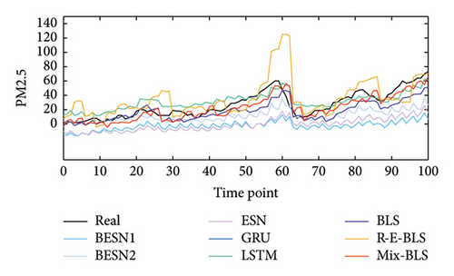
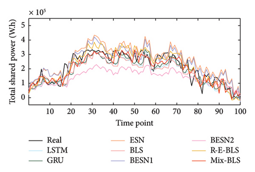
From the prediction result graphs, the Mix-BLS model can fit the changing trends of the real data well on both datasets compared to the comparative models. In Figure 5, during the first 30 time points with relatively mild trend changes, BLS, BESN-2, and Mix-BLS demonstrate more accurate prediction accuracy than other models, indicating the excellent predictive performance of the broad fusion network in multidimensional time-series prediction tasks. From the 30th to the 60th time points, the overall trend of the data shows a complex nonstationary sequence. R-E-BLS and Mix-BLS in the broad fusion network show remarkable learning capabilities, with significantly better prediction results than the comparative models. In the last 40 time points, the data trend displays strong volatility as nonstationary data. At this stage, the Mix-BLS model not only captures the underlying patterns of the data but also achieves smaller prediction errors. In Figure 6, the Mix-BLS model demonstrates its robustness in predicting wind turbine power data across a larger order of magnitude. It accurately fits the real data for the initial 30 time points. Notably, between the 70th and 100th time points, where the data exhibit more pronounced fluctuations, the Mix-BLS model not only maintains a significant accuracy advantage over the comparative model but also outperforms it. Conversely, during the period from the 30th to the 70th time points, where the trend changes are less pronounced, the Mix-BLS model still exhibits higher prediction accuracy than the comparative model. Compared to R-E-BLS, Mix-BLS demonstrates lower prediction errors and can manage complex multidimensional time-series prediction tasks requiring higher accuracy. Overall, from the perspective of prediction results, only Mix-BLS excels in conducting the multifaceted time-series prediction task.
Boxplots can reflect the central tendency and dispersion range of a set or multiple sets of continuous quantitative data distributions. Boxplots of the prediction results for the PM2.5 data and wind turbine power dataset are shown in Figures 7 and 8, respectively.
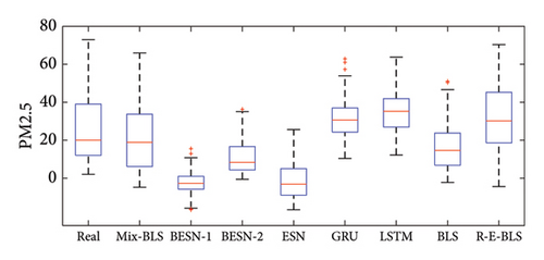
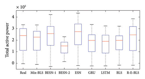
Boxplots can be used to compare the predictive performance of models from multiple dimensions. In a boxplot, the median of the dataset is denoted by a red line, while the edges of the box represent the upper and lower quartiles, and the whiskers represent the maximum and minimum values. The height of the box reflects the extent of data fluctuation to some degree. From the boxplots, it can be observed that the wind turbine power dataset exhibits more noticeable volatility compared to the PM2.5 dataset, as indicated by the height of the boxes, with a larger range between the maximum and minimum values and a higher median represented by the red line compared to the PM2.5 data. Figure 7 reveals that the BESN-1 model exhibits the smallest box plot, suggesting minimal variability in its predictions, which leads to a more concentrated representation of the information. However, this model’s predictions do not align closely with the data. The Mix-BLS model and the R-E-BLS model have boxes that are close to the real data. However, the Mix-BLS model’s predictions for the PM2.5 dataset exhibit the greatest alignment with the variability observed in the real-world data when contrasted against the other comparative models. In terms of data distribution and median values, the Mix-BLS model performed the best among all comparisons and had the best predictive ability. Figure 8 illustrates that the extreme values of predictions by Mix-BLS, LSTM, and BLS are near the actual data. However, the lower quartile of the LSTM predictions and the upper quartile of the BLS predictions are noticeably more distant from the actual data compared to the Mix-BLS model. Secondly, both R-E-BLS and Mix-BLS closely resemble the appearance of the real data in the boxplot. However, the spread between the highest and lowest values for the R-E-BLS model surpasses that observed in the real data. Accuracy and reliability in wind power prediction are crucial for the wind energy industry’s operation, management, and decision-making. Therefore, overall, only Mix-BLS meets the requirements.
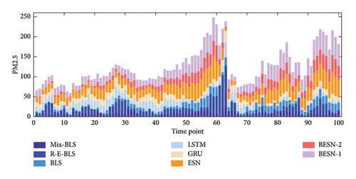
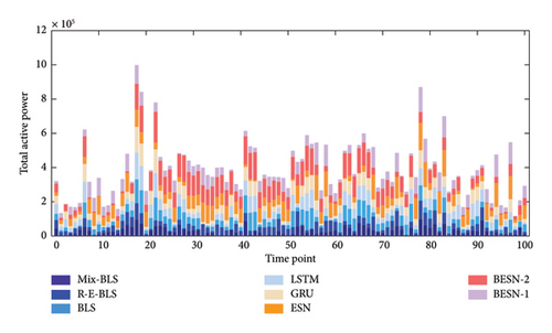
The absolute error stacking plots for the other model predictions on the two datasets are shown in Figures 9 and 10 to compare the prediction results of different models visually. These figures demonstrate that the Mix-BLS model consistently exhibits lower absolute errors compared to the other models at the same time points, reflecting superior prediction accuracy. Specifically, the absolute error of the Mix-BLS model is markedly lower than that of both the ESN and BESN-1 networks. This proves that a single ESN network has insufficient capability when dealing with complex multidimensional time-series prediction tasks and capturing the intricate patterns of real data. Furthermore, in the wind turbine power dataset, which exhibits considerable data fluctuations, the comparative models generally show larger absolute errors owing to the complexity of the multidimensional time series. In contrast, the Mix-BLS model consistently maintains the smallest absolute error. The Mix-BLS model proves stable prediction performance on datasets with more noticeable gradual changes in data trends.
Scatterplots allow for a more visual characterization of changes in the data. The absolute error scatterplots for the prediction results of the two datasets are presented in Figures 11 and 12, respectively. Different colors distinguish the various models; the horizontal axis represents the time steps, while the vertical axis indicates the true values of the absolute prediction errors corresponding to each time step.
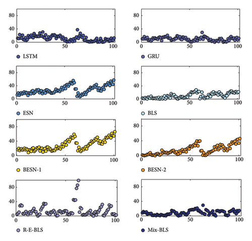
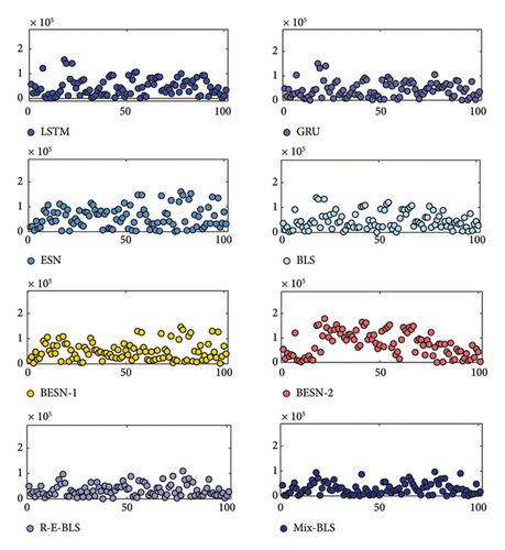
In Figure 11, the absolute errors of the prediction results for different models are predominantly concentrated below 40. The four models—LSTM, ESN, BESN-1, and BESN-2—exhibit a higher frequency of error fluctuations at the corresponding time steps compared to Mix-BLS. Additionally, the simple deep networks and broad networks demonstrate instability in multistep prediction tasks. Regarding prediction accuracy, the overall distribution of absolute errors from Mix-BLS is closer to zero, with reduced volatility in the error scatter, thereby offering a significant advantage in both stability and predictive performance. It is clear from Figure 12 that compared to the absolute error scatterplot in Figure 11, the order of magnitude of the error is larger because the order of magnitude of the real data on power loads is approximately in the hundreds of thousands. In the multistep prediction task of the wind turbine power dataset, the absolute error scatter of Mix-BLS is also more concentrated than that of the comparison model, and the overall distribution in the graph is closer to 0, which shows that Mix-BLS also performs stably and has excellent prediction accuracy in the face of more complex wind turbine power data.
In the experiments for predicting two multidimensional time-series datasets, single neural networks (including LSTM, ESN, GRU, and BLS) and broad fusion networks (including BESN-1, BESN-2, and R-E-BLS) were compared to better prove the predictive capabilities of the models. The prediction indicators for each model are shown in Table 2.
| Dataset | Model | SMAPE | MAPE | RSE | RRMSE | R | Time (s) |
|---|---|---|---|---|---|---|---|
| Fangshan air dataset | BESN-1 | 0.8089 | 1.4172 | 1.6605 | 2.5921 | 0.5866 | 18.5188 |
| BESN-2 | 0.2880 | 0.5934 | 0.6923 | 1.0204 | 0.7215 | 32.0712 | |
| ESN | 0.5770 | 0.9958 | 1.0724 | 1.5722 | 0.6631 | 13.9234 | |
| GRU | 0.3101 | 1.5526 | 0.6651 | 0.4826 | 0.7250 | 105.1334 | |
| LSTM | 0.3281 | 1.7615 | 0.7609 | 0.4928 | 0.7167 | 123.3598 | |
| BLS | 0.2939 | 1.3385 | 0.5357 | 0.5625 | 0.7226 | 11.0955 | |
| R-E-BLS | 0.2339 | 0.6397 | 0.5142 | 0.7210 | 0.7618 | 23.9234 | |
| Mix-BLS | 0.2817 | 0.5471 | 0.2396 | 0.4137 | 0.9035 | 22.1821 | |
| Wind turbine power dataset | BESN-1 | 0.4500 | 15.6391 | 0.5616 | 0.4202 | 0.8393 | 17.0139 |
| BESN-2 | 0.4621 | 10.9893 | 0.4503 | 0.6330 | 0.7650 | 37.6798 | |
| ESN | 0.4499 | 15.1139 | 0.5776 | 0.4187 | 0.8450 | 14.4588 | |
| GRU | 0.3993 | 6.5436 | 0.2885 | 0.4475 | 0.8490 | 95.0971 | |
| LSTM | 0.4152 | 6.6124 | 0.3282 | 0.5173 | 0.8403 | 113.4004 | |
| BLS | 0.4065 | 9.4641 | 0.2879 | 0.4460 | 0.8480 | 12.0503 | |
| R-E-BLS | 0.4232 | 8.8057 | 0.1732 | 0.2906 | 0.9266 | 33.9358 | |
| Mix-BLS | 0.4036 | 6.9252 | 0.1620 | 0.2971 | 0.9242 | 28.3342 | |
- Note: The bold values mean the results of the proposed method in this paper.
Table 2 shows that on the Fangshan dataset, Mix-BLS reduces 0.53% and 0.30% in SMAPE compared to BESN-1 and ESN, respectively. In terms of MAPE, it decreases by 1.01% and 1.21% compared to GRU and LSTM, respectively. Furthermore, it shows 0.61, 0.15, and 0.31 reductions in RRMSE compared to BESN-2, BLS, and R-E-BLS, respectively. The highest value achieved in the R indicator is 0.90. It also requires less training time. On the wind turbine power dataset, Mix-BLS demonstrates reductions of 8.7139%, 4.0641%, and 8.1887% in MAPE compared to BESN-1, BESN-2, and ESN, respectively. It also shows 0.1265, 0.1662, 0.1259, and 0.0112 reductions in RSE compared to GRU, LSTM, BLS, and R-E-BLS, respectively. Mix-BLS exhibits higher prediction accuracy than the comparative models, achieving desirable values in five indicators: SMAPE, MAPE, RRMSE, R, Time etc. The model error is smaller, and the predicted values are more correct. Furthermore, the broad learning architecture facilitates rapid updates of the network’s weight and bias parameters, leading to marked enhancements in the model’s predictive accuracy and a reduction in the duration required for training. Although the training duration of the Mix-BLS model may not be the most expedited, it attains the superior prediction accuracy by trading a modest increment in time for a significant enhancement in precision. Mix-BLS is an improvement over BLS by changing the mapping and enhancement layers. By comparing Mix-BLS with broad fusion networks, it proves better performance, indicating that the Mix-BLS network possesses the advantages of a broad network and exhibits superior predictive capabilities.
5. Discussion and Conclusions
Multivariate time-series data are highly complex, containing nonlinear and temporal components. Traditional time-series models can effectively handle the nonlinear aspects of multivariate time-series data, while deep learning networks can flexibly handle the time component, but with the increase in the number of network layers and the number of nodes in the hidden layer, it will bring the problems of slow training speed and easy to fall into the local extreme value. Compared with deep networks, broad networks can simplify the parameter tuning and reconstruction process and use pseudo-inverse solutions to update the weights quickly. It has the advantages of incremental learning, fast training speed, and generalized approximation ability, but a single broad network may not achieve the best results. Compared to a single neural network using a generalized learning framework, a fusion network can map complex multivariate time-series data to high-dimensional data through feature mapping and augmentation. This allows for the extraction of more time-series features to train the model. To this end, this paper proposes the Mix-BLS model to decompose complex multivariate time-series data into nonlinear and temporal data, combining the advantages of depth and breadth. The algorithm uses RBM and mapping functions at the mapping layer for feature learning and generation of mapping nodes. The enhancement layer uses echo state networks and gated loop units to process the data.
Experimental verification of the model’s performance was conducted on the Fangshan dataset and the wind turbine power dataset. The fusion network proved significant advantages over comparative models, including single neural networks (such as LSTM, ESN, GRU, and BLS) and broad fusion networks (such as BESN-1, BESN-2, and R-E-BLS). This advantage was particularly evident in the metrics of prediction accuracy. The Mix-BLS model reduced numerical values in model prediction error indicators and achieved a higher degree of fit with real data, achieving the desired prediction effect. The weight and bias parameters in the network of the broad learning architecture are updated faster, resulting in faster prediction speed compared to the comparative models. With shorter training time, the model’s prediction performance is greatly improved. By combining the characteristics of linear prediction models and nonlinear prediction models within a broad framework, the fusion network integrates the advantages of deep learning and traditional time-series models. This enhances the applicability of time-series prediction and achieves higher accuracy. Moreover, it can prove stable prediction performance in complex multidimensional time series with varying patterns.
While the current research has yielded promising results, the broad network exhibits certain limitations in the prediction of multidimensional time-series tasks, warranting further investigation, refinement in subsequent studies, and imbalanced learning [50, 51]. The Mix-BLS model does not fully consider the spatiotemporal characteristics of the data. In future research, a scalable model based on graph neural networks could be designed to enhance the understanding of deep relationships in multivariate time-series data, thereby expanding its applicability in practical applications [52]. In scenarios where the network encounters data loss or is constrained by limited data availability [53, 54], the optimization of network performance presents a promising avenue for future investigation. Furthermore, the stochastic nature of weight initialization in broad networks, encompassing connections between the input layer and feature mapping nodes, as well as between mapping and augmentation nodes, necessitates the development of more rational and interpretable initialization strategies. Such strategies are vital to mitigate the potential accumulation of random errors. Future research avenues could encompass the exploration of data-driven initialization techniques and the application of optimization algorithms to ascertain optimal weights.
Conflicts of Interest
The authors declare no conflicts of interest.
Funding
This study received funding from the National Key Research and Development Program of China (2022YFF1101103), MOE (Ministry of Education in China) Project of Humanities and Social Sciences (22YJCZH006), and National Natural Science Foundation of China (62203020, 62173007).
Open Research
Data Availability Statement
The data that support the findings of this study are available from the corresponding author upon reasonable request.


