Automatic Identification and Counting of South African Animal Species in Camera Traps Using Deep Learning
Abstract
In the area of ecology, counting animals to estimate population size and types of species is important for the wildlife conservation. This includes analysing massive volumes of image, video or audio/acoustic data and traditional counting techniques. Automating the process of identifying, classifying and counting animals would be helpful to researchers as it will phase out the tedious human–labour tasks of manual counting and labelling. The intention of this work is to address manual identification and counting methods of images by implementing an automated solution using computer vision and deep learning. This study applies a classification model to classify species and trains an object detection model using deep convolutional neural networks to automatically identify and determine the count of four mammal species in 3304 images extracted from camera traps. The image classification model reports a classification accuracy of 98%, and the YOLOv8 object detection model automatically detects buffalo, elephant, rhino and zebra school mean average precision of 50 of 89% and mean average precision of 50–95 of 72.2% and provides an accurate count over all animal classes. Furthermore, it performs well across various image scenarios such as blurriness, day, night and images displaying multiple species compared to the RT-DETR model. The results of the study display that the application of computer vision and deep learning methods on data-scarce and data-enriched scenarios, respectively, can conserve biologists and ecologists an enormous amount of time used on time-consuming human tasks methods of analysis and counting. The high-performing deep learning models developed capable of accurately classifying and localising multiple species can be integrated into the existing conservation workflows to process large volumes of camera trap images in real time. This integration can significantly reduce the manual labour required for labelling and counting, improve the consistency and speed of wildlife surveys and enable timely decision-making in habitat protection, population assessment and antipoaching initiatives. Additionally, these automated identification techniques can contribute towards enhancing wildlife conservation and future studies.
1. Introduction
Camera traps are commonly used in ecological studies to analyse animal behaviour and calculate densities, relative abundance or habitation in single and multispecies research [1]. Images obtained from camera traps have become increasingly significant and necessary in ecological management studies due to their ability to closely monitor animal activity and behaviour [2]. South Africa has an extensive and diverse biodiversity and a long history of wildlife conservation management. Monitoring biodiversity and ecosystems is important for South Africa—a biological diverse nation with various mammal species that are endangered by anthropogenic activities including poaching, hunting and climate change. Like other African nations, South Africa lacks sufficient information on the conservation of various species, and 17% of the mammal species are endangered and threatened with extinction [3].
In response to addressing the above challenges, the network called Snapshot Safari (https://www.snapshotsafari.org) was formed. Snapshot Safari is an extensive international trap network that was created to explore and track the biodiversity and ecology processes of animals in eastern and southern Africa [3]. Snapshot Safari is one of the biggest camera trapping networks in the globe. However, there is little information available on the conservation status of several species, and some South African regions lack core biodiversity data required to evaluate the success of ongoing conservation [4], with systematic long-term monitoring patterns of various species and populations essential for making informed decisions. However, the amount of data collected by camera traps has increased much to a point that it requires technical capacity to analyse such enormous datasets. Due to the enormous amount of image data produced by camera traps, the application of artificial intelligence (AI) for analysing images using machine learning (ML)/deep learning (DL) has received a lot of interest recently.
The study aims to contribute to the ML/DL (a computer science division) research domain by developing a species identification model [5] for biodiversity monitoring in South Africa. The objectives of this work are to conduct an investigation on image classification models for biodiversity using DL in, develop an automated image classification model for biodiversity monitoring using DL methods and evaluate the performance of the DL models. The investigation on developing a species identification model will contribute to the subject matter and the body of knowledge. Implementing the latest state-of-the-art image classification and detection methods in biodiversity monitoring as a strategy to tackle the issues that result from employing traditional ways of extracting information through human–labour is both a creative and an imperative effort [6]. Traditional methods for animal species detection and counting, such as manual observation and labelling, are often time-consuming, labour-intensive and prone to human error, especially when dealing with large volumes of camera trap images or video footage. Manual counting can suffer from inconsistencies due to observer fatigue, varying expertise levels and subjective biases. Additionally, manual approaches are not scalable to the increasing size of ecological datasets generated by automated monitoring systems [6, 7]. With the disadvantages led by traditional ways [7], the study will approach the concerns of wildlife conservation (area of application) using DL mechanisms [8]. As a result, this constitutes the research’s primary contribution of developing a DL model to identify, count and classify animal species in camera trap images to be employed for wildlife conservation.
ML, a subset of AI, can accomplish tasks without explicit programming for the related solution [9, 10]. Alternatively, it gains knowledge from prior instances of the same task through a series of processes referred to as training. Computer vision (CV) is a discipline within computer science, which focuses on collecting information from images and videos [11–13]. In the engineering domain, its aim is to automate operations analogous to those performed by the human visual system [5]. As a result, CV primarily involves creating artificial systems designed to address specific visual challenges, and as such, it employs techniques related to image processing and analysis [11]. Moreover, it is closely related to other fields such as ML and image recognition.
DL, a branch of AI and ML that includes training artificial neural networks (ANNs) to learn patterns from massive datasets [14]. DL is an expansion of frequently used ANNs, which are mathematical models influenced by the learning algorithms observed in biological neural networks, such as the central nervous system found in animals, specifically their brain [15]. DL mechanisms for image processing include the extensive architectures such as convolutional neural networks (CNNs) [9]. CNNs are significant mechanisms in DL, especially in the domain of CV. CNNs are particularly engineered to analyse grid-like data, such as imagery data, by harnessing the strength of convolutional layers and providing capabilities that conventional ways cannot provide [10].
CNNs present a category of neural networks mainly recognised for their efficiency in handling image and video data [15]. The first notable practical of CNNs appeared with the development of LeNet [15] or recognising handwritten digits. However, regardless of these early achievements, the extensive adoption of CNNs did not gain momentum until significant advancements in parallel computing systems converged with different new methods for effective training. After a period, a pivotal moment occurred in the year 2012 when Krizhevsky et al. [16] made a significant contribution to the well-known ImageNet Large Scale Visual Recognition Challenge (ILSVRC). Their introduced CNNs, referred to as AlexNet secured victory in the competition by lowering the classification error rate from 26% to 15%. Subsequently, in the following years, various architectures continued to advance, including renowned ones such as EfficientNet [17], visual geometry group network (VGGnet) [18] and residual network (ResNet-50) [19].
The motivation of this work was driven by the recent growth and interest in monitoring wildlife biodiversity or population monitoring for maintaining ecological balance, protecting endangered species and ensuring long-term sustainability for South Africa’s biodiversity and natural resources [8]. To achieve this, image classification and object detection will be performed to identify and count animals from imagery data acquired from camera traps, addressing the problem that arises with traditional methods used for biodiversity monitoring. Moreover, this will minimise the dangers that lie with ecological imbalances, as it will help in avoiding human–wildlife conflict and overpopulation of some species or depletion of food resources. By implementing an effective monitoring system, conservationists and authorities can make informed decisions regarding habitat protection, population control measures and conflict resolution strategies. In addition, management of animal species guarantees the monitoring and equilibrium of species within the ecosystem.
2. Related Literature
Pardo et al. [3] have studied 31 areas in South Africa with the aid of the Snapshot Safari—South Africa network, 21 of these areas are permanent grids for continuous monitoring. In total, 1408 cameras have been deployed for grids at fixed positions, while 83 have been installed at roaming locations. The use of camera traps has become vital in conservation management. Camera traps are essential for wildlife conservation in South Africa, as they enable researchers and conservationists to gather important data on the presence, abundance and behaviour of species in their natural habitats [6, 20]. Although there are many advantages of camera traps [21], managing the amount of human–labour needed to process, analyse and study large volumes of data is difficult. Norouzzadeh et al. [22] stated that the significance of possessing comprehensive and current knowledge about the location and behaviour of animals in the natural environment could enhance the ability to study and conserve ecosystems.
CV techniques have advanced lately, especially in the creation of You Only Look Once (YOLO) versions [23–26]. These versions combine localisation and target classification, which significantly increases detection performance [27, 28]. As a result, thanks to developments in CV technology, the field of wildlife detection is quickly becoming more data-rich and has been used to automatically identify a wide range of wildlife species [22, 29–31]. In a similar manner, different DL approaches such CNNs [22], ResNets [19], RetinaNets [32], and Faster R-CNNs [33] have proven to be highly accurate in object localisation and can be used as a dependable and consistent model for automated wildlife detection. When using DL models, researchers often trade interpretability for higher performance, as these models rely on increased abstraction through deeper architectures and end-to-end training. For example, deep ResNets, which can exceed 200 layers, have achieved state-of-the-art results across various complex tasks. However, their depth and integration make them inherently difficult to interpret. This has led to growing interest in finding a balance between model accuracy and interpretability. To address this, Zhou et al. [34] introduced class activation mapping (CAM)—a technique designed to highlight the regions of an image that a specific type of CNN (one without fully connected layers) uses for classification. CAM prioritises model transparency by simplifying the architecture slightly, thereby making it easier to understand the decision-making process at the cost of some performance.
Recently, there has been a significant academic interest in end-to-end transformer-based detectors (DETRs) primarily due to their simplified design and removal of manual elements [35–41]. However, their intensive computational demands limit their applicability for object detection. To overcome this computational bottleneck, the real-time detection transformer (RT-DETR) [42] was introduced. RT-DETR offers adaptable speed adjustments to suit different real-time situations without requiring retraining, courtesy of the DETR’s architecture. This makes the RT-DETR a groundbreaking real-time end-to-end object detection model that is a high-level performer in object detection.
3. Materials and Methods
3.1. Dataset
The study uses various South African Wildlife datasets acquired from open-source repositories such as the LILA repository (https://lila.science/datasets) and Kaggle (https://www.kaggle.com/datasets/biancaferreira/african-wildlife). The camera trap datasets such as the Snapshot Kruger, Snapshot Mountain Zebra, Snapshot Camdeboo and Wild Animals Facing Extinction are provided by the LILA repository and the African Wildlife Dataset from Kaggle. With a focus on four individual species such as buffalo, elephant, rhino and zebra, this work used a total of 3304 images from all the datasets, with each class consisting of 826 images and 826 text files. In the final dataset, the text files use YOLO annotation format, necessitating the construction of an object detection model. Figure 1 shows the overview of the image dataset employed in this study.
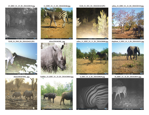
In this work, the data underwent random splitting that divided the dataset into three sets, namely training (70%), validation (20%) and testing (10%) for use during the experimental phase. To maintain consistent statistical allocation when splitting the data, K-fold cross-validation was implemented. Cross-validation, a data resampling technique, used to evaluate the generalisation performance of ML/DL models and to avoid overfitting [22]. In this work, the k-value was set to 5 because image classification models (especially CNNs) are computationally expensive to train. Training the model 5 times (once per fold) is often computationally feasible [16, 18, 22, 23]. The dataset summary after the data splitting phase for image classification and object detection models has the outcome of the animal classes for the respective data subsets as shown in Table 1. The total sum of images for each set includes 2312 images for training, 660 images for validation and 332 images for the test set. The dataset was partitioned in a manner that would test the prediction capabilities model in complex scenarios that include more than one animal class shown in the image.
| Dataset summary | |||
|---|---|---|---|
| Image classification and object detection | |||
| Class | Train | Validation | Test |
| Buffalo | 578 | 165 | 83 |
| Elephant | 578 | 165 | 83 |
| Rhino | 578 | 165 | 83 |
| Zebra | 578 | 165 | 83 |
| Total | 2312 | 660 | 332 |
3.1.1. Methods
In this study, the first phase was conducted by employing various data augmentation techniques to prepare data for experimentation and prediction using the proposed CNN architectures. These CNN architectures are tailored to execute image identification tasks through the fine-tuning of parameters and integration with state-of-the-art regularisation techniques. The study used three distinct CNN architectures, namely EfficientNet-B3, VGG-16 and ResNet-50, for the image classification and YOLOv8 and a transformer-based RT-DETR Large for object detection. Moreover, the gradient-weighted class activation mapping (Grad-CAM) was used to improve the model interpretability.
3.1.2. Data Augmentation
Image augmentation is a method that artificially creates diverse variations of input images, effectively encompassing a wide spectrum of potential alterations [43]. By incorporating augmentation, the model will be exposed to a broad array of transformations during the training stage, allowing it to learn and recognise objects in different forms and shapes [44]. Furthermore, this method enhances the model’s capabilities for generalisation, allowing it to make accurate predictions even on unobserved images belonging to the target classes [45].
The critical step in building an optimal model for species identification lies in the preprocessing phase. Using augmentation, the model was fed with a variety of transformations so that it learns features in various forms during the training phase [44]. This approach assisted in enhancing the generalisation ability of the models to predict unseen images of target classes [45]. Furthermore, it aided in minimising the risk of overfitting. Two augmentation toolkits were used, given that classification tasks were performed using both Keras and PyTorch. Augmentation was performed using the Torchvision library [43] in python for data manipulation to enhance model training of EfficientNet-B3 and ResNet-50 architectures, while the Keras was used to augment data for the VGG-16 architecture. The reason behind using the Torchvision library in PyTorch is that it augments and manipulates data for training the EfficientNet-B3 and ResNet-50 models, ensuring efficient integration with the training pipeline and compatibility with the architecture requirements. In parallel, Keras’ ImageDataGenerator was utilised to perform augmentation for the VGG-16 model, offering a straightforward and flexible approach consistent with the Keras environment. This dual-toolkit approach was selected to maximise model performance while maintaining compatibility and efficiency within each framework’s workflow.
3.2. Image Classification
This research aims to identify animal species harnessing extensive DL methods to tackle the challenge of processing vast amounts of data to enhance conservation management. Conducting image classification experiments by integrating transfer learning with CNNs enhances performance in a different and unaccustomed task by leveraging previously acquired knowledge from related tasks. This technique has proven to be exceptionally beneficial in the context of species image analysis, tackling the issues that arise with using limited data and computational resources. However, it is worth taking note that in several studies [9, 16, 30, 33], the configuration of transfer learning has been applied to address problems outside the species identification spectrum, thus making it a reliable approach.
3.2.1. EfficientNet-B3 Architecture
In the domain of deep convolutional neural network (DCNN) architecture, EfficientNet holds a distinguished position [16], owing to its cutting-edge achievements in the fields of image recognition and classification. EfficientNet [17] is a family of CNNs that has drawn notice for its effectiveness and superior performance in image classification applications. EfficientNet [17] is a family of CNNs that has drawn notice for its effectiveness and superior performance in image classification applications characterised with escalating levels of depth, width and resolution; each model in the EfficientNet series includes starting from EfficientNet-B0 to EfficientNet-B7, which signifies a distinct scale of the model architecture [46]. In summary, the EfficientNet models offer a variety of choices with various levels of precision and computational demands. Depending on the application requirements and resource availability, users can select the suitable model.
In this work, EfficientNet-B3 was the variant selected and employed from the EfficientNet range. The reason behind using this specific version of EfficientNet is due to the balanced combination of computational efficiency and accuracy [17]. EfficientNet-B3 introduces a crucial advancement through the employment of a compound scaling technique, which dynamically adjusts the model’s architecture by increasing both depth (quantity of layers) and width (quantity of filters) in proportion to the resolution of the input image [47]. Due to this adaptability, the model can process a variety of image dimensions efficiently, which in turn improves performance and effectiveness for a wide range of image processing tasks. Figure 2 illustrates the design of the EfficientNet-B3 model.
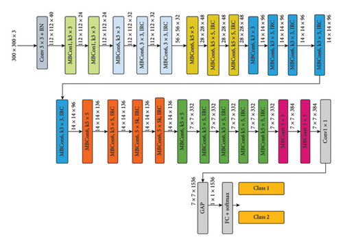
The network’s first layer, which is the initial CNN layer, considers an input image with a three-dimensional structure and a size of 300 × 300 pixels. The EfficientNet-B3’s design (illustrated in Figure 2) consists of several CNN layers. There are layers of flattening, dropout (using a dropout rate of 0.3), and a dense layer used for predictions after the training phase. There are ∼11 million parameters in the model in total.
3.2.2. VGG-16 Architecture
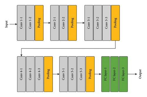
In this study, researchers employed a pretrained VGG-16 CNN model [18]. This model was fine-tuned by freezing certain layers to mitigate overfitting. Granted that the dataset employed in this study is too small. The VGG-16 model consists of 16 convolutional layers. As shown in Figure 3, the input image for this network possesses a dimensionality of (224 × 224 × 3) and consists of 16 convolutional layers with a fixed-size filters of (3 × 3) and 5 max-pooling layers with a size of (3 × 3) throughout the entire network. At the top, the network integrates two fully connected layers together with a softmax output layer. The VGG-16 model is employed in this study based on that it is considered as an extensive network, encompassing approximately 138 million parameters [18, 22]. Its framework comprises multiple stacks of convolutional layers to develop DCNNs that excel at gathering hidden features. Furthermore, VGG-16 was selected for its simplicity and well-established performance in image classification tasks. Its uniform architecture of stacked convolutional layers makes it a suitable benchmark for comparison. The architecture of the VGG-16 network is illustrated in Figure 3.
3.2.3. ResNet Architecture
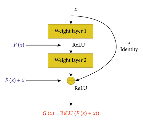
The current configurations of the neural network designs construct layers to approximate some mapping function from an input image to a target specified as H(x) [19]. Fundamentally, it approximates the residual of this function that can be considered as F(x) = H(x) − x. To recover the original function, one simply adds the residual back to in a form of input: F(x) + x. Fundamentally, these layers are referred to as residual blocks are given a task to estimate the residuals and then re-insert the immediate input to reconstruct the actual target function.
As shown in Figure 4, the architecture of this block features a skip connection within the network. This skip connection incorporates adding the input of stacked layers to the output of the same stack of layers. It is imperative to note that F(x) and x may not have the same dimensionality, requiring a linear projection to match the dimensions of the original input x. This concept of residual learning has led to the enhancements of different ResNet-based models, which vary in the quantity of layers and compositions of building blocks. These networks employ residual blocks, whereby each possesses a skip connection incorporated within their framework. Notable examples include ResNet-34 and ResNet-50 networks, which employ distinct types of residual blocks. However, this work will employ the ResNet-50 model from the extensive ResNet architecture range due to its balance of accuracy and computational efficiency [19, 22, 29, 30]. The following section discusses the object detectors proposed in this study.
3.2.4. Grad-CAM
To enhance the interpretability of the classifiers used in this study, we employed Grad-CAM [63]. Grad-CAM is a method that generates class-discriminate localisation heatmaps by employing the gradients of the target class streaming into the last convolutional layer to generate a weighted combination of feature maps. The resulting heatmap for a given class c is calculated as , where Ak depicts the kth activation map and represents the importance weight for that feature map, derived from the gradient . This method was crucial in identifying the regions within input images that contributed most to the model’s decision-making process.
3.3. Object Detection
As stated in Section 3.1.1, the study will conduct experiments by performing image classification and object detection tasks. In this section, researchers delve into the framework of the object detector proposed in this study. In the domain of DCNNs, YOLO is a widely established object detection algorithm. YOLO comprises multiple iterations, with each successive version building on the previous version and the RT-DETR’s extensive design that was built on the multilayer decoder of the DETR equips it to address object detection tasks. In this study, researchers focused on the use of particularly YOLOv8 and RT-DETR large models as the selected object detectors. The details of the selected object detectors are elaborated in the section below.
3.3.1. The YOLOv8 Algorithm
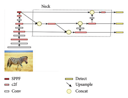
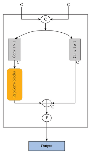
YOLOv8 [49] shows an advanced version of the YOLO framework. It is developed through the integration of foundational approaches offered in YOLOv4 [26]. It incorporates components such as the cross-stage partial (CSP) approach from Wang et al. [50], the fusion of path aggregation network (PAN) [51] and feature pyramid network (FPN) [52] which is widely referred to as the PAN-FPN, as well as the spatial pyramid pooling fast (SPPF) module. YOLOv8 encompasses distinct-scale models grounded on scaling coefficients, a feature inspired by YOLOv5 to accommodate diverse requirements of different tasks. While maintaining the fundamental concepts of YOLOv5, the YOLOv8 integrates the coarse-to-fine (C2F) module [53] that is inspired by the efficient layer aggregation network (ELAN) concept in the architecture of YOLOv7 [54]. Components that make up the architecture of the YOLOv8 include the input, backbone, neck and the output. The Yolov8 was used in this study for its balance of speed and accuracy, making it well-suited for real-time applications. It incorporates improvements in feature extraction and bounding box regression, as well as support for anchor-free detection and adaptive training strategies. The architecture of the YOLOv8 network is illustrated in Figure 5.
3.3.2. The RT-DETR Large Algorithm
RT-DETR comprises a backbone, an efficient hybrid encoder and a transformer decoder with supplementary prediction heads [35]. Figure 6 provides an illustration of the RT-DETR architecture. The RT-DETR architecture involves input features from the final three backbone stages [42] into the encoder. The hybrid encoder converts features at various scales into a series of image features by using cross-scale feature fusion and intrascale feature interaction [41]. Subsequently, the uncertainty-minimal query selection is used to choose a set number of features to serve as initial object queries for the decoder [41, 42, 55]. Lastly, the decoder repeatedly refines object queries to generate bounding boxes and classes with the help of supplementary prediction heads. The RT-DETR was selected based on its representation of a shift towards transformer-based object detection, offering a fully end-to-end detection pipeline without the need for hand-crafted components such as anchor boxes or nonmaximum suppression.
3.4. Computational Resources
Both classification and object detection models were coded using Python programming language. Table 2 shows the hardware and environment parameters.
| Parameters | Configuration |
|---|---|
| CPU | 13th Gen Intel Core (TM) i7-13700F |
| Operating system | Windows 11 |
| Python Version | 3.11.4 |
| Torch | 2.0.1 |
3.5. Model Evaluation
A DL model undergoes an evaluation process to assess its algorithmic performance. The selection of performance metrices varies depending on the task performed and dataset used. In the context of classification tasks, metrics such as accuracy, precision, recall (sensitivity) and F1-score will be employed. Meanwhile, for the object detection task, researchers will use evaluation metrices such as precision, recall, intersection over union (IoU) and mean average precision (mAP).
Accuracy is outlined as the proportion of correct predictions out of the total predictions made [56]. However, high accuracy results do not guarantee that the model is optimal, particularly when conducting experiments on imbalanced datasets. To guarantee model performance, researchers will employ various other metrices like precision, recall and F1-score.
The use of a confusion matrix is a well-known approach to assess the performance of individual classes within classification models. It allows for a detailed comparison of the quantity of correctly and incorrectly predicted instances for every class in the model. Furthermore, in the confusion matrix, the rows symbolise the predicted class instances, whereas the columns symbolise the actual class for those instances. Table 3 shows the confusion matrix structure.
| Prediction results | |||
|---|---|---|---|
| Positive (PP) | Negative (PN) | ||
| Actual observation | Positive (P) | True positive (TP) | False negative (FN) |
| Negative (N) | False positive (FP) | True negative (TN) | |
True positives (TPs) describe correctly predicted instances of the positive class, whereby the predicted result aligns with the actual positive class. In a similar manner, true negatives (TNs) denote instances that were correctly predicted of the negative class. Then, false positives (FPs) correspond to instances that were incorrectly predicted as belonging to the positive class, meaning the predicted result is different from the expected outcome. Lastly, like the FPs, false negatives (FNs) are instances that were inaccurately predicted as part of the negative class [58].
This section details the research methodologies, delineating the steps required to achieve the research goals. The study utilised the South African Wildlife image dataset sourced from Kaggle, containing four unique mammal species. Data augmentation techniques were applied to prepare the images, and distinct CNN architectures such as the EfficientNet-B3, VGG-16, and ResNet-50 models were employed for the classification task. The performance outcomes from the experiments were assessed in the following section using a confusion matrix for classification models and assessment metrics like precision, recall, IoU, and mAP for object detection tasks which were performed using YOLOv8 and RT-DETR Large models.
4. Results
During experimentation, the issue of working with a small dataset was eminent, so it required techniques that will assist classifiers with knowledge and equip models with the fundamental mechanisms to carry out the related tasks. Prior to training, image samples were pre-processed through the employment of distinct data augmentation tool to encourage variety of image perspectives for DL techniques. During model training, the transfer learning approach was implemented to aid in providing necessary assistance by allowing models to serve as established feature extractors through the replacements of final layers. This improves the model’s capability within reduced training time. The results of image classification and object detection tasks are presented in the subsequent chapters.
4.1. Image Classification
Several hyperparameters were fine-tuned to construct an optimal model, these included batch size, number of epochs, learning rate, dropout, and optimiser. The dropout layers used in the experimentation incorporated values of 0.3, 0.4, and 0.5. With EfficientNet-B3 results accomplished using a dropout of 0.3 across the CNN layers, VGG-16 architecture used a dropout of 0.5 following convolutional layers and 0.3 following FC layer, and ResNet-50, employed 0.4 across CNN layers. For PyTorch model architectures, which included EfficientNet-B3 and ResNet-50, the Cross-Entropy Loss [60] and Negative Log-Likelihood function [33] were used to compile their architectures, respectively. EfficientNet-B3 used stochastic gradient descent (SGD) optimiser [61] and ResNet-50 employed the ADAM optimiser [62], while VGG-16 was compiled with categorical cross-entropy loss function and RMSprop was employed as the optimiser. The learning rate of 0.0001 was used for all models. The batch size was 50 for all models. Moreover, the hyperparameter permutations of CNN classifiers performed in this study are outlined in Table 4. Subsequently, the results are displayed using the learning curve, classification report and confusion matrix.
| Model | Hyperparameter | Configuration |
|---|---|---|
| EfficientNet-B3 | Epoch | 50 |
| Batch size | 50 | |
| Learning rate | 1e − 4 | |
| Optimiser | SGD | |
| Loss function | Cross-entropy loss | |
| VGG-16 | Epoch | 50 |
| Batch size | 50 | |
| Learning rate | 1e − 4 | |
| Optimiser | RMSprop | |
| Loss function | Categorical cross-entropy loss | |
| ResNet-50 | Epoch | 50 |
| Batch size | 50 | |
| Learning rate | 1e − 4 | |
| Optimiser | Adam | |
| Loss function | Negative log-likelihood loss | |
4.1.1. Learning Curve
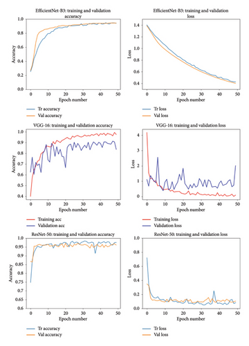
Learning curves in the context of CNNs are visual representations that show how a DL model performs over a period when it is trained on a train set [32]. The training and validation accuracy will be measured to assess the models’ accuracy of accurately predicting instances on the training and validation datasets as well as the number of samples that were classified correctly by the model. The training and validation loss assesses the error between predicted and actual values in the training set as well as the how good does the model generalises to the data points that unseen during training. The loss played a critical role in evaluating the models’ ability to execute accurate predictions on new and unseen data. In this study, the curve against the number of epochs with an object to observe training progress of each model throughout the stated number of epochs was plotted.
Figure 7 depicts the loss and accuracy curves of the diverse CNN classifier models. The graphs show that the training patterns are largely similar across all models, although there are some minor variations. This visualisation offers a comprehensive comparison among different types of CNN classifier models. The accuracy curves do not display much of overfitting since the validation curve aligns with the training curve. Furthermore, an assessment of the loss curves reveals a consistent decline towards a minimal value, with the validation loss curve starting to decrease after the fifth epoch and continuing until the end of the plot. In the case of the overall training and validation processes of the models, the curves maintained a relatively stable learning process.
4.1.2. Classification Report
The EfficientNet-B3 model achieves an accuracy rate of 96.25%, with a precision of 96.26%, a recall of 96.25% and an F1-score of 96.23%. Meanwhile, the VGG-16 model attains an accuracy of 81.88%, a precision of 81.88%, a recall of 86.73% and an F1-score of 83.64%. Additionally, the ResNet-50 model demonstrates an accuracy of 98.13%, a precision of 98.26%, a recall of 98.13% and an F1-score of 98.14%. These models also exhibit notable precision, recall and F1-scores. Detailed results for all classification models across the four animal classes can be found in the classification report outlined in Table 5, offering valuable insights into the efficacy of various CNN architectures for species classification. These performance metrics enable researchers and practitioners to compare and assess model performance, aiding in the selection of the most appropriate architecture for species classification tasks.
| Model | Class (species) | Precision | Recall | F1-score |
|---|---|---|---|---|
| EfficientNet-B3 | Buffalo | 0.95 | 0.93 | 0.94 |
| Elephant | 0.97 | 0.97 | 0.97 | |
| Rhino | 0.97 | 0.95 | 0.96 | |
| Zebra | 0.95 | 1 | 0.98 | |
| Accuracy | 0.96 | |||
| Macro-F1 | 0.96 | 0.96 | 0.96 | |
| Weighted-F1 | 0.96 | 0.96 | 0.96 | |
| VGG-16 | Buffalo | 1 | 0.42 | 0.60 |
| Elephant | 0.86 | 0.90 | 0.88 | |
| Rhino | 0.66 | 0.97 | 0.79 | |
| Zebra | 0.95 | 0.97 | 0.96 | |
| Accuracy | 0.83 | |||
| Macro-F1 | 0.87 | 0.82 | 0.81 | |
| Weighted-F1 | 0.87 | 0.82 | 0.81 | |
| ResNet-50 | Buffalo | 0.99 | 0.95 | 0.97 |
| Elephant | 0.99 | 1 | 1 | |
| Rhino | 0.93 | 1 | 0.96 | |
| Zebra | 1 | 0.97 | 0.99 | |
| Accuracy | 0.98 | |||
| Macro-F1 | 0.98 | 0.98 | 0.98 | |
| Weighted-F1 | 0.98 | 0.98 | 0.98 | |
4.1.3. Confusion Matrix
The confusion matrix serves as a standard method to evaluate the classifier’s performance, representing the accurate predictions of positive samples among the total collected samples [56]. The proposed CNN classifier models notably achieved accurate predictions for most samples within the 160-sample test set from the wildlife dataset. This success can be attributed to the diverse image perspectives facilitated by the transform functions within the augmentation techniques and the extensive transfer learning mechanisms employed. Resulting to enhanced predictions compared to other advanced DL models, the effectiveness demonstrated by CNN classifiers renders them increasingly reliable and robust for multiclass classification of animal species using camera trap images.
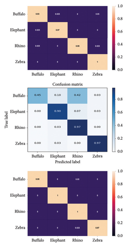
The performance of EfficientNet-B3, VGG-16, and ResNet-50 for the classification task is visually depicted through confusion matrices in Figure 8. EfficientNet-B3 notably exhibits higher accuracy for the Zebra class (Figure 8; EfficientNet-B3: Confusion matrix), followed by the elephant, rhino and buffalo classes, respectively. The few misclassification instances observed in the buffalo, elephant and rhino classes have minimal impact on overall predictions. Notably, the zebra, rhino and elephant species achieved correct predictions of over 90%, while the Buffalo class a 45% correct prediction rate (refer to Figure 8; VGG-16: Confusion matrix). VGG-16 performs well overall, with occasional misclassifications primarily in the Buffalo class, where some samples are predicted as the Rhino species class. On the other hand, ResNet-50 (Figure 8; ResNet-50: Confusion matrix) attains higher accuracy for wildlife animal species like the elephant and rhino, reducing misclassifications among these species and performing commendably on the other species, namely Buffalo and Zebra. Additionally, ResNet-50 significantly enhances classification accuracy across most animal classes, especially considering a substantial number of training samples and a limited number of samples in testing (see Figure 8), surpassing other CNN classifiers. Consequently, ResNet-50 demonstrates robustness in handling species mixing and exhibits superior tree species classification capabilities.
EfficientNet-B3’s performance of 96.25% accuracy on the South African Wildlife dataset is indeed impressive, especially compared to VGG-16. It demonstrates the effectiveness of EfficientNet models in handling large-scale classification tasks with diverse image qualities, including those involving animal species. This highlights the advancements in model architectures like EfficientNet in achieving competitive recognition performance across various domains.
The VGG-16 performed well, whereby both learning curves showed a good fit but with minor inconsistencies. This model performed well on unseen data because of the high validation accuracy and low validation which are vital signs that symbolise good generalisation results. The minor inconsistencies were reflected extensively in the confusion matrix whereby the overall prediction of the four distinct species was good, but there were some misclassifications of species. Misclassifications included minor instances of buffalo samples predicted as elephant or rhino and elephants predicted as rhino. While VGG-16 is effective, it is relatively shallow and parameter-heavy compared to modern architectures like ResNet or EfficientNet. It might fail to abstract enough semantic differences between visually similar animals. However, it did not affect the overall outcome of the predictions. The ResNet-50 architecture was employed in this study for the classification experiments. For the classification task, ResNet-50 performed quite better than the EfficientNet-B3 model. The results of the ResNet-50 model were also shown using the learning curve and confusion matrix to analyse performance for distinct animal species that were predicted.
The ResNet-50 model performed well, indicating that the size of the architecture and the parameters were a good fit for the task with the least misclassifications. The model demonstrated minimal challenges during predictions among the species in the test dataset. Among the four animal species, overall predictions displayed relatively better performance, and this is evident in the models’ performance on the train, validation and test sets shown in Table 6. The models achieved the desired level of accuracy, and ResNet-50 particularly stood out compared to the EfficientNet-B3 and VGG-16 models.
| CNN model performance (accuracy) | |||
|---|---|---|---|
| Model | Training (%) | Validation (%) | Testing (%) |
| EfficientNet-B3 | 96.31 | 94.44 | 96.25 |
| VGG-16 | 95.36 | 83.68 | 82.49 |
| ResNet-50 | 98 | 96.18 | 98 |
The image classification predictions were conducted randomly among the four classes in the test set, and the first prediction which was tested on the EfficientNet-B3 which performed well. The VGG-16 was implemented on a different package and trained faster compared to other architectures. However, with an accuracy of 81.88%, behind the 98.13% of the ResNet-50 and the 96.25% of the EfficientNet-B3 architectures, respectively, it still performed well on the validation and testing datasets. Making the ResNet-50 stand out among all classifiers that were employed for image classification in this study. The following sections illustrate the classification sample predictions and succeeded by the results of object detection models.
4.2. Sample Predictions for Species Classification
4.2.1. EfficientNet-B3
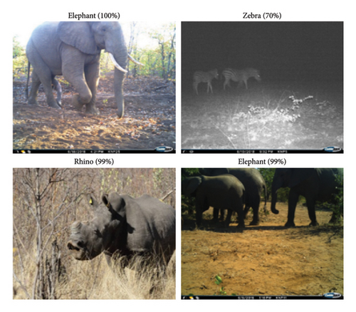
The sample predictions were performed randomly on the test set among the four animal species to determine how the CNN classifiers perform on unseen set of images in terms of correctly classifying the true species. EfficientNet-B3 model trained well and generated good results enabling it to classify animal species. Figure 9 shows the classification outcome of EfficientNet-B3 on the four animal classes.
4.2.2. VGG-16
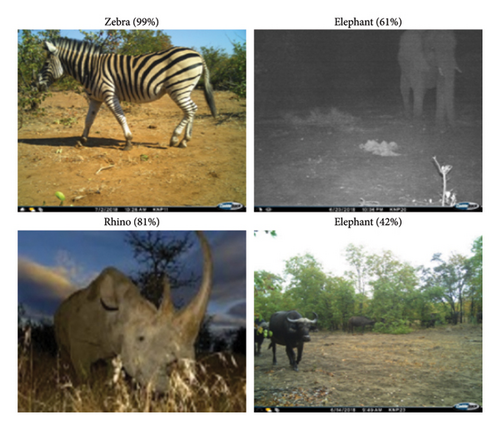
The VGG-16 model trained well granted its varied accuracy on predicting positive observations (recall) on the among the four classes. Nonetheless, the VGG-16 prediction capability was still accurate even on the buffalo class, enabling it to classify animal species. Figure 10 shows the classification outcome of VGG-16 on the various animal classes.
4.2.3. ResNet-50
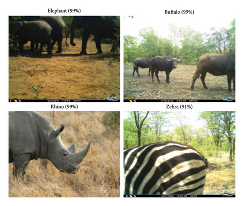
The best overall CNN classifier was the ResNet-50. The ResNet-50 model performed well, indicating a well-structured architecture for the classification task, with only minimal misclassifications. This model had the least challenges during predictions among the species in the test dataset compared to other classifiers. Figure 11 shows the classification result of the ResNet-50 model on the different animal classes.
4.3. Grad-CAM Activation Maps
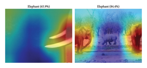
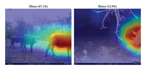
The Grad-CAM visualisations reveal key insights into the limitations of the underperforming models, particularly in their ability to localise and attend to discriminative features during species classification. In the elephant images, while high-confidence predictions (e.g., 96.7%) show focused attention on relevant body parts like the legs and torso, lower-confidence predictions (e.g., 65.9% and 73.9%) highlight a reliance on partial features such as tusks or include diffuse attention across both the animal and the background that led to a misclassification by predicting “elephant” instead of buffalo. Notably, the second-row images (84.4%), the model predicts “elephant” despite a clearly visible rhino in the centre, indicating confusion when multiple species appear within the same frame. Similarly, in the rhino images, one instance is misclassified due to the model focusing on the hindquarters of a buffalo, while another true rhino detection receives a low-confidence score (33.9%) as the model attends more to the background and only a small portion of the rhino’s head. These examples suggest that the model often fails to consistently capture the most informative features, especially under challenging conditions such as occlusion, poor contrast or species co-occurrence. The heatmaps expose the models’ sensitivity to irrelevant regions and partial cues, which contributes to its reduced generalisation performance. Figure 12 highlights the Grad-CAM visualisations.

4.4. Object Detection
This section presents the performance of the object detection model based on the validation and test sets. The following subsections provide a comprehensive evaluation of the object detection model’s performance and sample predictions for each animal class, buffalo, elephant, rhino and zebra.
4.4.1. Bounding Box Analysis
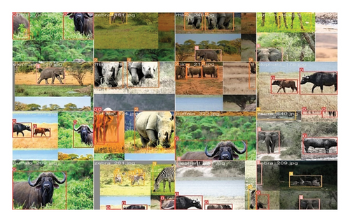
A bounding box aids in defining a precise spatial location for a predicted object. Provided that the study uses YOLO annotation format, this means that an individual predicted object confined within a bounding box is described by five attributes: −x, y, w, h and confidence. The x and y values depict the centre coordinates of the box regarding the position of the cell’s box. In a case where the centre falls outside a cell, that cell will not represent it since it is not responsible for that centre. Each cell is associated with only objects whose centres lie within it. Figure 13 shows the image objects with the corresponding bounding boxes for each animal class.
Here, represents the confidence score in the ith grid of the jth bounding box. Pi,j represents a function that depends on the presence of an object. If there is an object on the ith grid of the jth of the box, then the Pi,j = 1; otherwise Pi,j = 0. The term IoUtruthpred denotes the IoU between the ground-truth box and the predicted bounding box.
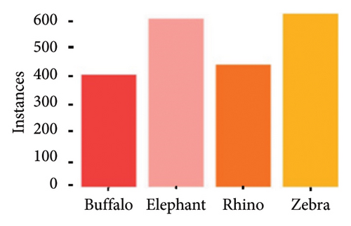
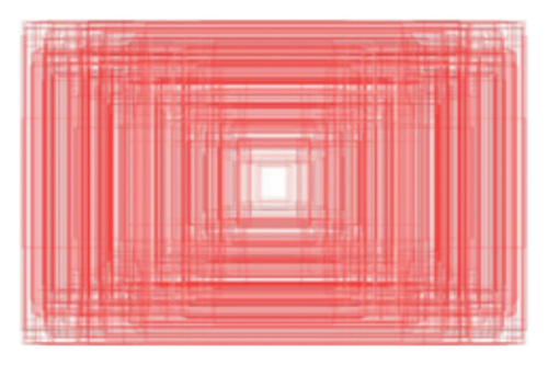
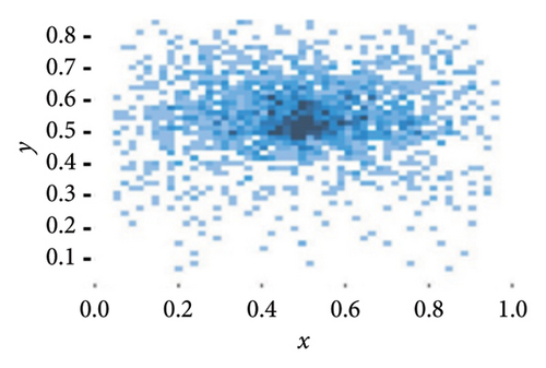
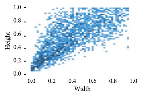
The subfigures in Figure 14 are presented in a left-to-right, top-to-down order. Figure 14(a) illustrates the object distribution in the dataset, revealing that zebras and elephants are the predominant objects. Figure 14(b) shows the sizes of the object bounding boxes, with the centre coordinates of all object boxes fixed at one point. This signifies that the dataset contains a significant number of small-sized objects. Figure 14(c) illustrates the dispersion of centre point coordinates for the object bounding boxes, demonstrating an even concentration of object centres across the image area. Figure 14(d) is a scatter plot depicting the width and height of the object bounding boxes, with the darkest regions in the bottom-left corner, emphasising the predominance of small objects in the dataset.
For object detection, various hyperparameters were configured to construct the YOLOV8 and RT-DETR large detector models. The primary training hyperparameters are consistent across both the original YOLOv8 and RT-DETR large models. Training was performed on the wildlife dataset using these models, employing AdamW [54] as the optimiser with a learning rate of 0.01, an IoU threshold of 0.5, and a confidence score of 0.01. The default settings are maintained for batch size and workers, while the epochs are set to 100 due to the dataset’s scale. Table 7 provides an overview of these main training hyperparameters.
| Object detection model hyperparameters | |
|---|---|
| Hyperparameter | Configuration |
| Epochs | 100 |
| Optimiser | AdamW |
| Learning rate | 0.01 |
| IoU threshold | 0.5 |
| Confidence score | 0.01 |
| Batch size | Default |
4.4.2. Object Detection Evaluation
The study employed YOLOv8 and RT-DETR models for the object detection tasks using the camera trap images from the South African Wildlife Dataset. The selected object detection models underwent a final evaluation on the unseen test set to assess their performance. The YOLOv8 achieved a precision of 0.815, a recall of 0.869, an mAP50 of 89% and an mAP50-95 of 72.2%. The RT-DETR achieved a precision of 0.891, a recall of 0.817, an mAP50 of 84% and a mAP50-95 of 71.4%. The models demonstrated strong performance on the challenging structure of the test set, which allowed single- and multiple-object detection tests to be conducted. However, due to variations in class instances, some classes performed slightly poorly in the test set. This decline in performance was due to the differences between the test set images and those in the training and validation sets. Detailed model performance for each class is outlined in Table 8.
| Precision | Recall | mAP50 (%) | mAP50-95 (%) | ||
|---|---|---|---|---|---|
| YOLOv8 | Testing (all) | 0.815 | 0.869 | 89 | 72.2 |
| Buffalo | 0.933 | 0.629 | 79 | 68.1 | |
| Elephant | 0.675 | 1 | 93.4 | 84.8 | |
| Rhino | 1 | 0.973 | 99.5 | 80.8 | |
| Zebra | 0.651 | 0.875 | 83.9 | 55.1 | |
| RT-DETR | Testing (all) | 0.891 | 0.817 | 84 | 71.4 |
| Buffalo | 0.935 | 0.654 | 0.752 | 63.1 | |
| Elephant | 0.966 | 1 | 0.995 | 91.7 | |
| Rhino | 0.917 | 0.8 | 0.797 | 72.2 | |
| Zebra | 0.756 | 0.812 | 0.831 | 58.6 |
4.4.3. Species Detection and Counting
At this stage, the YOLOv8 and RT-DETR large models underwent adequate training using the training set that equipped them with necessary information and patterns to perform predictions on the test set.
To assess the predictive capabilities, the models were tested across all four classes of animals, including images containing multiple animal species of different classes. This evaluation aimed to determine whether the models exhibit robust detection abilities, even in scenarios where the image contains multiple animals of different species and features. Moreover, the prediction results provided a count for each species detection in the image. Figures 15 and 16 show the detection of the object detectors on images that comprise various animal classes, and this was done to determine the models’ capabilities in detecting and counting animal species.
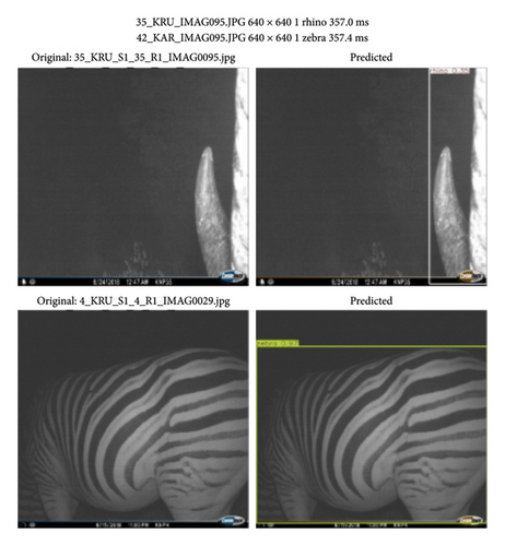
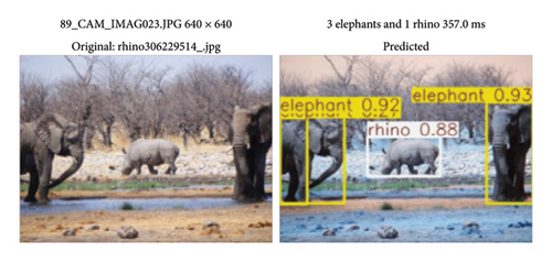
The object detection models show great detection capabilities with accurate species counts, especially on a complex test set that was partitioned in a manner that will require the models to detect multiple species in one image.
The results in Figure 17 illustrate a comparison between YOLOv8 and RT-DETR in detecting wildlife under low-light, nighttime conditions. YOLOv8 successfully detected a buffalo with a confidence score of 84.3% in a grayscale image, demonstrating its ability to handle challenging lighting scenarios and maintain reasonable accuracy. In contrast, RT-DETR failed to detect any animals in a similar nighttime scene, despite the presence of multiple visible subjects. This suggests that YOLOv8 is more robust in extracting features under poor illumination, likely due to its convolution-based architecture being better suited for low-level texture and edge detection. RT-DETR, relying heavily on global context through transformer mechanisms, may struggle in such conditions where contrast is low and object boundaries are less defined. These results highlight a potential limitation of RT-DETR in real-world deployment where nighttime images are common and emphasise the practical strength of YOLOv8 in low-light wildlife monitoring applications.
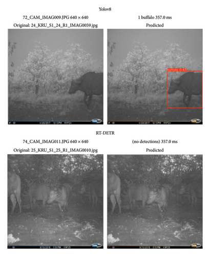
This highlights YOLOv8’s stronger capability to recognise objects in low-contrast, grayscale images typical of nighttime wildlife monitoring. In comparison with the YOLOv8, the RT-DETR large model offers higher precision, making it more suitable for small dataset applications. During the training phase, the current RT-DETR large model trained faster than the YOLOv8 model. However, the RT-DETR large model trained thus far is not optimised for rapid deployment on large-scale datasets. This limitation arises from the study’s focus on only four animal species within the training set that led the model to have a slightly lower recall and mAP, making YOLOv8 the better object detector model. To address this, for deployment in wildlife conservation projects, researchers must expand the training dataset to encompass a broader range of animal species. This expansion will enable us to enhance the recall and mAP of the RT-DETR large model, empowering it to detect a more extensive array of animal species efficiently.
5. Discussion
This work was linked to a study by [33], which used RetinaNet to identify animals in images. In their study, they used 561 images from three species classes, and their proposed model generated an accuracy of 77% on the test and 86% on their best performing animal class of elephant. Norouzzadeh et al. [23] conducted a study on automatic image classification using multitask models and were able to accurately classify images of animals with a classification accuracy of 93.8%. Similar to their research was the study by Gomez et al. [63], which analysed DNNs on the SS dataset. They primarily conducted the task of identifying the species, while Norouzzadeh et al. [23] additionally attempted to count animals, assess their behaviour and determine whether there was presence of the offspring. With focus on the species identification tasks conducted by the two studies [23, 63], the performance of their networks was 92.0% and 57%, respectively.
The previous studies emphasised on the poor image quality that led to a low generalisation by the model. In this study, low quality was not predominant and with the number of images that were used led to a higher mAP in the test set. The proposed object detection models detect and count four animal classes of mammal species. The models were applied on 1504 camera trap images and generated adequate results on the object detection task. The YOLOv8 model yielded a precision of 0.815, a recall of 0.869, an mAP50 of 89% and a mAP50-95 of 72.2% on the test set. The second object detector model that was employed in the study is the RT-DETR large. The RT-DETR large generated a precision of 0.891, a recall of 0.817, an mAP50 of 84% and a mAP50-95 of 71.4%. This means that YOLOv8 consistently demonstrated strong detection capabilities, particularly under challenging conditions such as nighttime imagery, where it was able to accurately detect and localise animals with high confidence. Its convolution-based architecture, optimised for spatial feature extraction and real-time inference, makes it well-suited for detecting objects in low-light environments and cluttered scenes. In contrast, RT-DETR underperformed in similar settings, often failing to detect animals in grayscale or low-contrast images. This limitation is likely due to its transformer-based architecture, which depends heavily on global context and may struggle when object boundaries are unclear, or lighting is poor. Overall, YOLOv8 proved to be more robust and practical for real-world wildlife monitoring tasks, particularly in variable lighting conditions where reliable detection is critical.
Primarily, these findings demonstrate that biologists and ecologists may be able to conserve a significant amount of time by using standard CV techniques and DL in both data-scarce and data-enriched scenarios. Instead of manually searching through vast amounts of images to identify, count, and classify animal species, this significant portion of manual labour that tends to be tedious could be applied towards more crucial scientific endeavours. We granted that the study focused on identifying and counting four animal species in South Africa. For future studies, more animal species in South Africa will be targeted for biodiversity monitoring. Ultimately, the automated counting techniques described in this paper have the potential to significantly enhance both wildlife conservation and future research.
The results acquired from the DL model, opened significant diversifications in accuracy, precision, recall, mAP50, mAP50-95 and F1-scores across different class, because of the hereditary differences in the detection complexities. Furthermore, it is imperative to take note of the choice of parameter selection that was implemented in this study was based on the restricted investigation within the realm of parameters. This restriction was driven by the limitations of the computational resources. An expansion of these resources would allow a more extensive investigation for optimal parameter configurations. For example, this will enable investigations on a broader spectrum of values for key parameters such as batch size and learning, as well as other model accuracy determinants such as dropout rates and the number of epochs. It is worth noting that improving a wider range is not only applicable to hyperparameter permutation but the data as well.
We granted that image data used in this study consisted of 3304 images for both classification and object detection tasks, which was insignificant based on some CNN models in several classes. Moreover, increasing the number of data includes employing more than four animal classes and as well as the incorporation of using video data as part of the dataset. In this manner, the model will be exposed to a wide variety of data and will be able to learn more animal features due to the distinct perspective it provides. Making it a clear indicator that significantly expanding the training and validation data stands a high chance to yield improved model performance.
Dataset repository such as the Labelled Information Library of Alexandria: Biology and Conservation (LILA) is benchmark dataset that provides a variety of images that contain various objects and backgrounds. Moreover, these images capture images found within nature reserves across South Africa which provide real-world research scenarios pertaining to monitoring that will address conservation challenges tailored for a specific nature reserve which has its unique terrain, biomes and resources. Making it suited for research methods to be conducted on South African soil.
6. Conclusion
This paper addresses the challenge of manual counting animals in camera trap images by developing two distinct automated identification solutions, a DL image classification model and an object detection model. The dataset applied in this paper had several minor complexities, given that the collected imagery data provided unsubstantial volumes of images. Additionally, the image data consisted of few low-quality images, and images were some animals were small in blurry conditions. All these issues affected the clearness of the image. Furthermore, some images had several extra animal species within them. Therefore, this dataset presented a challenge that required more complex techniques such as DL, which provided an iterative process, an advanced method of parameter permutation to generate optimal prediction results. However, the difficulty of this approach requires complex computational resources to withstand thousands of distinct image features with hours of training. The goal of the image classification models was to analyse image data by establishing a set of target classes and then use unseen images to train the models for identification. The results from the models were accessible for acquisition and interpretation. For a small experimental testing sample of four classes of mammal species, the classification model produced good prediction results, with 98% accuracy by ResNet-50, the best performing model for the predicted label corresponding to the truth label. Additionally, Grad-CAM visualisations were used to interpret and explain the prediction behaviour of the models. These visualisations provided valuable insights into the regions of interest the models relied on when making decisions, particularly in cases of misclassification. The results revealed that the underperforming models often focused on irrelevant background areas or nondistinctive features, which contributed to incorrect predictions, especially between visually similar species such as buffalo and rhino. This analysis not only supported the quantitative findings but also highlighted the importance of integrating explainability tools in wildlife monitoring workflows to improve model transparency and trustworthiness. The data collected for use in this research were gathered with the goal of performing object detection and image classification of animal species in camera trap images. The dataset consists of four animal classes commonly found in nature reserves around South Africa; these include buffalo, elephant, rhino and zebra. However, the research can be expanded, and the principles used in this study can be conducted on other studies related to wildlife conservation and ecology. In furtherance of that, with this research using four animal classes, conducting research that will include other animal classes will open innovative ideas in conserving wildlife. Moreover, future research efforts should consider the development of different models such as Inception (Google Net), MobileNet and hybrid transformer detection models tailored for various animal classes to optimise the detection performance for specific and multiple class scenarios.
Conflicts of Interest
The authors declare no conflicts of interest.
Author Contributions
The authors confirm contribution to the paper as follows: study conception and design: S.M., M.E. and I.C.O.; data collection: S.M.; analysis and interpretation of results: S.M., M.E. and I.C.O.; draft manuscript preparation: S.M., M.E. and I.C.O. All authors reviewed the results and approved the final version of the manuscript.
Funding
This research was funded by the Northwest University.
Acknowledgements
The authors thank the North-West University (NWU) for their kind financial assistance in the form of a bursary, which made it much easier for the authors to finish the research article. Without the wonderful assistance provided by NWU, this research would not have been possible. Their dedication to encouraging academic success and helping ambitious researchers has made a significant contribution to the project’s successful completion.
Open Research
Data Availability Statement
The data that support the findings of this study are openly available in LILA repository https://lila.science/datasets and Kaggle https://www.kaggle.com/datasets/biancaferreira/african-wildlife/code.


