Topological Sequences Connected With Inverse Graphs of Finite Flexible Weak Inverse Property Quasigroups: An Approach From Polynomials to Machine Learning
Abstract
Research on the confluence of algebra, graph theory, and machine learning has resulted in significant discoveries in mathematics, computer science, and artificial intelligence. Polynomial coefficients can be beneficial in machine learning. They indicate feature significance, nonlinear interactions, and error dynamics. Moreover, they empower models to extrapolate complex real-world data, facilitating tasks like regression, classification, optimized performance, and feature adaptation. The structural characteristics of flexible weak inverse property quasigroups are very close to the conventional group structures, and the class of these nonassociative groups plays an important role in real-time applications. This manuscript studies the relationship between topological sequences T(f) and inverse graphs of finite flexible weak inverse property quasigroups, and it presents a new computational framework with applications ranging from polynomials to machine learning. We define and analyze topological sequences based on the structural properties of quasi-inverse graphs. Polynomial representations are provided, allowing for a thorough algebraic approach of the topological properties of these graphs. In particular, the coefficients of these polynomials have been demonstrated to give important information for improving the predictive and explanatory capacity of machine learning models.
1. Introduction
Machine learning (ML) includes building models that can recognize relationships, associations, and trends in data. This includes the usage of mathematical functions for converting inputs to outputs, which is an effective tool for current analysis. Polynomial functions can be beneficial because of their simplicity as well as their capacity to detect complex situations [1, 2]. The coefficients of these polynomials are important for indicating the dynamics, variability, and usefulness of the ML model. They indicate the weights distributed to each term of the polynomial. They illustrate the effect of one particular input variable on the outcome. Changing these numbers allows the ML model to accurately represent linear and nonlinear high-order correlations, making polynomial functions essential for regression, classification, projection, and functionality transformation [3, 4]. Polynomial models in regression can illustrate nonlinear associations among input and output variables; however, kernel-based techniques leverage polynomial kernels for nonlinear data distribution in high-dimensional scenarios [5]. These algebraic structures constitute the foundation of several ML models since they facilitate a broad spectrum of interactions. This algebraic formula is versatile because the coefficients can be modified to correspond with any position or type of data. The values here are not solely mathematical constants, but also parameters which effect a model’s ability to standardize data.
In various ML applications, polynomial coefficients are employed to transform raw input data into exciting and effective features. For instance, the model input function will clarify a nonlinear relationship by expressing x to the standard basis {1, x, x2, …, xn} in polynomial representation. The degree of the polynomial is determined by its coefficients, and this influences the model’s flexibility. The high-degree model prefers a more sophisticated data model. Polynomial coefficients can represent feature relationships. For example, in a polynomial function, the term cijx1x2 represents the correlation between features x1 and x2, with cij denoting the intensity and direction of this correlation [6, 7]. In ML, the learning algorithm usually aims to optimize polynomial coefficients in order to minimize loss functions. This optimization aligns the model’s predictions to the actual outcomes, ensuring that the coefficients display meaningful relationships in the data. They are present in activation functions, basis functions, and curve fitting networks, which offer new characteristics to improve model performance. Higher order polynomials with many coefficients have a danger of overfitting the training data. Regularization approaches, such as ridge or lasso regression, address this by penalizing big coefficients. Large or small coefficient values in a large degree polynomial might cause calculation instability. Input scaling and the application of orthogonal polynomials resolve this problem. These principles, which range from object transformation to model accuracy optimization, serve as a bridge between mathematical theory and practical implementation. Thus, the logic and utility of polynomial coefficients enable researchers to set resilient, versatile, and interpretable ML models that can tackle a wide range of difficulties in a variety of industries [8–10].
The term “quasigroup” refers to a generalization of group structure that ensures a unique solution of equations and has applications in ML. Mathematical characteristics of quasigroups, such as nonassociativity and the presence of left and right inverses in some cases, make them useful in a wide range of applications where usual group structures may be insufficient. They play a crucial role in nonlinear and nonassociative data relations, as well as unique mapping. These algebraic structures might confront dataset constraints. Their nonassociative functionality facilitates the building of distinct data maps, which will assist in maintaining information by enhancing convenience diversity and data separation in the feature space for better categorization [11, 12]. Flexible weak inverse property quasigroups (FWIPQs) are frequently utilized due to their ability to take into account changes in complex maps and applications based on data. Weak inverse property presents many advantages in reverse items; it is vital for repetition algorithms, data storage, and erroneous correction methods. This approach is even more malleable thanks to its flexible property. This symmetry in flexible binary operations gives strength in quasigroup actions, making it an ideal tool for scenarios with nested or hierarchical settings. These two identities can be used to construct FWIPQs, which are algebraic structures that have special invertible and versatile properties [13, 14]. In ML, these mathematical mechanisms provide an adequate basis for dealing with challenging circumstances and unforeseen behaviors in the model. Their nonassociation ability double functionality gives them the ability to interact that cannot be portrayed via group or ring elements, while functional reversal contributes in learning and recurrent willingness to change. Plus, flexibility enables algebraic algorithms to be implemented in a wide range of ML models, involving monitored learning and graph-based approaches. These, for example, can be advantageous for algorithms, data generation, and convenience strategies because they allow input data to be transformed in innovative and adaptive ways. This is very handy when preserving unique data points, for instance in distribution processes or groups. Their objective is to advance graph-based ML through an exchange between civilizations. Creating this relationship with FWIPQs permits the ML system to gain a greater grasp of the graph’s content and underlying dynamics, allowing for more accurate estimations and detections. Finally, FWIPQ is an elegant algebraic strategy that is sufficient for ML advancement. Their particular qualities make them great for applications that require modeling, adaptable workflows, and flexibility. As research in this particular field continues, it will be applied more frequently, ultimately in a more effective and powerful ML algorithm. Leading algebraic systems enable an accessible and accurate method for studying abstract algebraic concepts and their interactions, making them highly beneficial in modern research [15–17].
Paulo Ribenboim was the very first mathematician to develop the concept of an involutorial graph, underlining how vital it is in figuring out the connections between graph theory and algebra [18]. He wrote that it is a simple graph that can be composed as the vertex set is the elements of the finite group and any two distinct vertices are adjacent if and only if their product is the involution. In ring theory, the involutory Cayley graph can be utilized to study the set of involutory elements in a ring. The involutory Cayley graph of a ring R is made up of vertices that symbolize the elements of R and edges that interconnect pairs of vertices whose difference corresponds to the set of involutory elements [19]. This theoretical framework has rendered it more straightforward to examine the algebraic and combinatorial properties of rings. But in case of inverse graphs of finite groups, the situation is totally different. An inverse graph is a type of simple graph where vertices represent the elements of a mathematical system and edges indicate a certain property based on binary operation of the structure [20–22]. In this graph, two distinct elements are adjacent only when their product is the noninvolution element of the group. This graph becomes especially useful in algebraic systems that include an inverse for each element, such as groups and rings [23, 24]. Inverse graphs represent incarnations and interactions, which makes quickly examining and handling algebraic conditions. These graphs are useful for understanding and assessing symmetry, duality, and structural interaction in algebraic systems. This graph shows the reverse connection between algebraic structures, plays an important role in ML, and can serve as a powerful motivator by taking advantage of symmetry, reversible, and structural properties [25, 26]. It is used to describe reversible behavior in the neural network, normalize the current, and perform graph-based tasks, including prediction and node classification. In the problems associated with optimization, inverse graph solutions indicate two contexts on the site, which help develop cost functions and limitations. They help with convenience technique by identifying the opposite addiction in data and contributing to the cementic ML by defining input–output and hidden space. In learning reinforcement, it represents reversible behavior on state transition diagrams, which improves system learning [27, 28]. In addition, inverse graphs are useful in the cryptographic system, as they help understand the reversible features that reduce encryption and decryption. Quantum ML represents transitions in a unique way and quantum functions which are invertible, and allows for more efficient circuit structure. These graphs improve the structural integrity of the flexible and explanatory ML models and ensure programming skills and theoretical approaches. In short, the versatility of inverse graph in applications such as cryptography, quantum computing, and optimization highlights their importance for advanced ML techniques.
This study of the topological sequences associated with the quasi-inverse graphs for finite FWIPQs appoints a new multidirectional research technique that combines abstract algebra, graph theory, and ML. By using the structural properties of such graphs, the study examines the complex link between algebraic symmetry and topological properties, which provides new insight into the behavior of FWIPQ. A significant contribution is modeling and analysis of these graphs with polynomial coefficient, which provides direct mathematical details on the underlying algebra. The topological sequences allow polynomial functions with geometric properties to quasi-inverse graphs. In addition, this algebraic and topological representation is expanded to the ML area, where they are used to identify patterns and classification of data. Mixing these graphs with ML reveals the efficiency of detecting structural models and predicting algebraic features. The task, which combines theoretical stiffness and practical implementation, provides insight into how topological and algebraic properties can lead to modern ML techniques. The relationship between FWIPQs and their quasi-inverse graphs paves the way to the new algorithm approaches that use structural efficiency and symmetry. Finally, this task provides a solid basis for future research on algebraic systems by identifying the potentially affected scientific domains.
2. Methodology
This study focuses on the class Ξ of FWIPQs, , where λ > 1 represents a positive integer with some conditions. In order to achieve our findings, we rely on polynomial coefficient techniques in ML, graph theoretic tools, and combinatorial approaches. Moreover, we implement vertex and edge partitioning methods, the polynomial approximation approach, analytical processes, and the degree computation method. Furthermore, technologies including MATLAB, 3D SURFACE PLOTTER, and CorelDRAW were used for producing the figures of this research. The following sequence depicts all of the steps involved in our approach:
Structural properties of quasi-inverse graphs of FWIPQs, in the class Ξ ⟶ introduction of some new definitions ⟶ topological sequences T(f) associated with quasi-inverse graphs ⟶ polynomial approximation method ⟶ graphical representations of polynomials and role of polynomial coefficients in ML.
3. Key Findings
- •
Some important structural results of have been computed. For example, quasi-inverse graphs of are always connected, not complete, and have diameter 2.
- •
Degree-based topological sequences T(f) and M-polynomials have been investigated in terms of λ and/or ϕ(λ), where ϕ denotes the Euler’s phi function.
- •
With the help of Lagrange’s interpolation method, we obtain polynomials PT(f)(x) of sequences T(f) under three different conditions applied on λ.
- •
2D and 3D geometrical representations of all polynomials have been provided in a broad manner.
- •
Polynomial coefficients derived from quasi-inverse graphs provide crucial algebraic and topological characteristics for finite FWIPQs.
- •
Polynomial coefficients are useful characteristics for training ML models because they provide precise predictions of FWIPQ properties like invertibility and flexibility.
4. Preliminaries
A mathematical object graph is the combination of two sets Θ, vertex set, and Υ, edge set, which can be denoted by Γ = (Θ, Υ) or simply Γ. Readers can see the book [29] for the basic definitions like finite graph, simple graph, connected graph, and complete graph. For any finite graph Γ, degree of the vertex μ ∈ Θ is the number of edges adjacent to μ and it can be denoted by d(μ). Let Γ be the connected graph, then the distance d(μ1, μ2) between two distinct vertices μ1, μ2 of Θ is the length of the shortest path between them. Moreover, minimum and maximum eccentricities of the graph Γ are taken as radius, rad(Γ), and diameter, diam(Γ), respectively, where ecc(μ1) = Max{d(μ1, μ2) : ∀μ2 ∈ Θ}. A multiplicative function can be taken as Euler’s totient function, where ϕ(λ) indicates the numbers which are less than as well as relatively prime to λ and is the set of positive integers. For example, ϕ(7) = 6.
Example 1. Let C3 be the cyclic group generated by β, then Table 1 indicates 9-order FWIPQ, .
| ⊙ | (e, 0) | (e, 1) | (e, 2) | (β, 0) | (β, 1) | (β, 2) | (β2, 0) | (β2, 1) | (β2, 2) |
| (e, 0) | (e, 0) | (e, 1) | (e, 2) | (β, 0) | (β, 1) | (β, 2) | (β2, 0) | (β2, 1) | (β2, 2) |
| (e, 1) | (e, 1) | (e, 2) | (β, 0) | (β, 1) | (β, 2) | (β2, 0) | (β2, 1) | (β2, 2) | (e, 0) |
| (e, 2) | (e, 2) | (β, 0) | (e, 1) | (β, 2) | (β2, 0) | (β, 1) | (β2, 2) | (e, 0) | (β2, 1) |
| (β, 0) | (β, 0) | (β, 1) | (β, 2) | (β2, 0) | (β2, 1) | (β2, 2) | (e, 0) | (e, 1) | (e, 2) |
| (β, 1) | (β, 1) | (β, 2) | (β2, 0) | (β2, 1) | (β2, 2) | (e, 0) | (e, 1) | (e, 2) | (β, 0) |
| (β, 2) | (β, 2) | (β2, 0) | (β, 1) | (β2, 2) | (e, 0) | (β2, 1) | (e, 2) | (β, 0) | (e, 1) |
| (β2, 0) | (β2, 0) | (β2, 1) | (β2, 2) | (e, 0) | (e, 1) | (e, 2) | (β, 0) | (β, 1) | (β, 2) |
| (β2, 1) | (β2, 1) | (β2, 2) | (e, 0) | (e, 1) | (e, 2) | (β, 0) | (β, 1) | (β, 2) | (β2, 0) |
| (β2, 2) | (β2, 2) | (e, 0) | (β2, 1) | (e, 2) | (β, 0) | (e, 1) | (β, 2) | (β2, 0) | (β, 1) |
Theorem 1 (see [44].)Let Cλ = <β; βλ = e> and be the λ−order cyclic group and 3-order group of residue classes, respectively. Then, the algebraic structure is the FWIPQ under the binary operation ⊙, which can be defined as follows: , where 0 < λ1, λ2 ≤ λ, , T1,2 = T2,1 = β, and Tm,n = e otherwise . We denote this class by Ξ.
Definition 1 (topological index). Let Ω be the collection of finite simple graphs such that Ωi∩Ωj = ∅, when i ≠ j and , where each subcollection Ωi contains only isomorphic graphs and i is taken from the indexing set {1, 2, 3, …}. We say a mapping defined by Ωi ↦ ρi, which is the topological index.
5. Main Results
Our main results are presented in the following sections. In the first section, we look at the structural results of quasi-inverse graphs. The next section covers the role of polynomial coefficients in ML using topological sequences.
Definition 2 (quasi-inverse graph). Let Q be the finite quasigroup. A simple graph ΓQ can be taken as quasi-inverse graph of Q when we have
- a.
All the elements of Q are the vertices of ΓQ.
- b.
Any two distinct vertices μ1, μ2 have an edge μ1μ2 in Υ if (μ1⊙μ2)⊙(μ1⊙μ2) ≠ (e, 0) or μ1⊙μ2 is the noninvolution of Q, where (e, 0) is the identity element of Q.
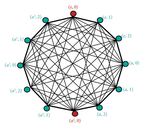
Example 2. For the 4-order cyclic group C4 generated by a, Figure 1 shows the quasi-inverse graph of order 12.
Definition 3 (topological sequence). Let Ω and S be the collection of all finite simple graphs and nonempty subsets of the set of positive integers, respectively. A map defined by |Ωi| ↦ ρi is called topological sequence associated with f.
Definition 4 (approximated curve). A 2D geometrical representation C(f) of PT(f)(x) is known as approximated curve, where polynomial PT(f)(x) can be obtained from the points (|Ωi|, ρi).
5.1. Structural Results of Quasi-Inverse Graphs
Theorem 2. Let be any FWIPQ of the class Ξ. Then prove that I = {(e, 0), (β(λ/2), 0)} is the set of involutions of .
Proof 1. Let be any involution of the quasigroup , where 0 < λ1 ≤ λ. Then,
It implies that 2λ1 = λ. Thus, for even order cyclic group Cλ, we have two involutions {(e, 0), (β(λ/2), 0)}. It completes the proof.
Theorem 3. Let In be the set of noninvolutions of the FWIPQ, with λ > 1. Then, is the connected graph.
Proof 2. Since the binary operation ⊙ between (e, 0) and any noninvolution of is again the same noninvolution, we can say that (e, 0) is adjacent to every element of In. Therefore, we have to only prove that every element of is adjacent to each noninvolution of In. If λ is odd, then there is nothing to prove. In the case of even λ, we have two involutions {(e, 0) and (β(λ/2), 0) by Theorem 2. Now, we consider the product , where . If . It means the right inverse of (β(λ/2), 0) is and can be written as . It is a contradiction to the fact that . Again, if . It gives , a contradiction. Thus, there is a path between any two vertices of the quasi-inverse graph . It completes the proof.
Theorem 4. With the help of same notations, the diameter of quasi-inverse graph is always 2.
Proof 3. By Theorem 3, the quasi-inverse graph is connected, so we are in the position to find it diameter. We consider the following vertex partitions Θ = {(e, 0)} ∪ In ∪ I, where I = (β(λ/2), 0) for even λ and I = ∅ for all λ and In is the set of noninvolutions of . Since every element in In is adjacent to (e, 0) and there is no edge between (e, 0) and the element of I, we have ecc((e, 0)) = 2. Also, for any element of In, we have as is not adjacent to its left or right inverse but adjacent to (e, 0) and element of I. Now we take (β(λ/2), 0) of I, and it follows from the construction and connectivity of quasi-inverse graph that (β(λ/2), 0) is not adjacent to (e, 0) but adjacent to every vertex in In. Hence, ecc((β(λ/2), 0)) = 2. Thus, , as required. It completes the proof.
Theorem 5. Let be the quasi-inverse graph with λ > 1. Then, we have the following assertions:
- a.
is not a complete graph.
- b.
has not isolated vertex.
Theorem 6. Let be the 3λ−order quasi-inverse graph with λ > 1. Then, the sum of degrees of its vertices is bounded above by
- a.
(3λ − 1)2 for odd λ.
- b.
9λ2 − 6λ + 2 for even λ.
Proof 4. Let Θ = {μ1, μ2, …, μ3λ} be the set of vertices of quasi-inverse graph. By the first theorem of graph theory, we have the following:
For odd λ:
For even λ:
It completes the proof.
5.2. Role of Polynomial Coefficients in ML
Theorem 7. Let p and be the positive integer and quasi-inverse graph, respectively, where λ = 4p. Then, we have the following degree-based topological sequences in terms of Euler’s totient function ϕ:
- 1.
T(M1) = 27λ3 − 54λ2 + 39λ − 10 + 6λϕ(λ) − 5ϕ(λ)
- 2.
T(M2) = (81/2)λ4 − 111λ3 + (207/2)λ2 − 33λ + 2 + (9/2)λ2ϕ(λ) − (9/2)λϕ(λ) + ϕ(λ)
- 3.
T(F) = 81λ4 − 222λ3 + (421/2)λ2 − (143/2)λ + 3 + 9λ2ϕ(λ) − 9λϕ(λ) + (3/2)ϕ(λ)
- 4.
- 5.
- 6.
T(RR2) = (ψ3(λ)/ψ4(λ))
- 7.
T(SDD) = (81λ4 − 216λ3 + (421/2)λ2 − (179/2)λ + 11 + 9λ2ϕ(λ) − 15λϕ(λ) + (11/2)ϕ(λ)/9λ2 − 15λ + 6)
- 8.
T(H) = (81λ4 − 213λ3 + 208λ2 − 92λ + 18 + 9λ2ϕ(λ) − 18λϕ(λ) + 9ϕ(λ)/54λ3 − 135λ2 + 111λ − 30)
- 9.
T(I) = (ψ5(λ)/ψ6(λ))
- 10.
T(A) = (ψ7(λ)/ψ8(λ))
Proof 5. Vertex set Θ and edge set Υ of can be partitioned as follows:
These partitions and equation (5) provide the following first Zagreb topological sequence as:
With the help of equation (6), second Zagreb topological sequence can be calculated as follows:
Equation (7) can be used to find the forgotten topological sequence in the form of Euler’s ϕ function as follows:
Following is the calculation of second modified Zagreb topological sequence by equation (4):
Polynomials ψ1(λ) and ψ2(λ) can be seen in Table 2. Equation (5) gives the generalized topological sequence at χ = 2 as follows:
Following lines show, with the help of equation (6), the inverse Randi ć topological sequence at χ = 2:
Table 2 provides the coefficients of polynomials ψ3(λ) and ψ4(λ). Following is the computation of symmetric degree topological sequence by equation (7):
With the help of equation (8), harmonic topological sequence can be calculated as follows:
Equation (9) can be used to find the inverse sum indeg topological sequence in the form of Euler’s ϕ as follows:
Tables 2 and 3 provide the polynomials ψ5(λ) and ψ6(λ), respectively. Following lines show, with the help of equation (10), the augmented Zagreb topological sequence:
Coefficients of ψ7(λ) and ψ8(λ) can be seen in Table 3. Similarly, we can obtain the other results. It completes the proof.
| Power of λ | ψ1(λ) | ψ2(λ) | ψ3(λ) | ψ4(λ) | ψ5(λ) |
|---|---|---|---|---|---|
| λ12 | — | — | — | 118,098 | — |
| λ11 | — | — | — | −1180,980 | — |
| λ10 | — | — | 6561 | 5,393,142 | — |
| λ9 | — | — | −49329 | −14,871,600 | — |
| λ8 | — | — | 167,670 + 729ϕ(λ) | 27,578,070 | — |
| λ7 | — | — | −(340,308 + 5832ϕ(λ)) | −36,231,300 | — |
| λ6 | 243 | 486 | 459,387 + 20,088ϕ(λ) | 34,578,090 | 243 |
| λ5 | −1035 | −2430 | −(434,907 + 38,988ϕ(λ)) | −24,154,200 | −1062 |
| λ4 | 1839 + 27ϕ(λ) | 5022 | 295,850 + 46,701ϕ(λ) | 12,256,920 | 1878 + 27ϕ(λ) |
| λ3 | −(1765 + 108ϕ(λ)) | −5490 | −(144,416 + 35,388ϕ(λ)) | −4406,400 | −(1698 + 81ϕ(λ)) |
| λ2 | 990 + 159ϕ(λ) | 3348 | 48,724 + 16,578ϕ(λ) | 1,065,312 | 813 + 90ϕ(λ) |
| λ1 | −(320 + 102ϕ(λ)) | −1080 | −(10,240 + 4392ϕ(λ)) | −155520 | −(190 + 44ϕ(λ)) |
| λ0 | 48 + 24ϕ(λ) | 144 | 1008 + 504ϕ(λ) | 10,368 | 16 + 8ϕ(λ) |
| Power of λ | ψ6(λ) | ψ7(λ) | ψ8(λ) |
|---|---|---|---|
| λ14 | — | 19,131,876 | — |
| λ13 | — | −250,840,152 | — |
| λ12 | — | 1,513,189,674 + 2,125,764ϕ(λ) | — |
| λ11 | — | −(5,557,829,661 + 23,383,404ϕ(λ)) | — |
| λ10 | — | 13,856,792,634 + 115,854,138ϕ(λ) | — |
| λ9 | — | −(24,741,983,709 + 341,047,341ϕ(λ)) | 1,259,712 |
| λ8 | — | 32,513,539,968 + 662,214,852ϕ(λ) | −13,226,976 |
| λ7 | — | −(31,793,047,398 + 889,435,404ϕ(λ)) | 61,620,912 |
| λ6 | — | 23,091,077,916 + 841,543,020ϕ(λ) | −167,174,280 |
| λ5 | — | −(12,272,191,578 + 558,909,720ϕ(λ)) | 291,057,624 |
| λ4 | — | 4,621,747,734 + 253,470,384ϕ(λ) | −337,247,064 |
| λ3 | 36 | −(1,160,249,805 + 73,363,104ϕ(λ)) | 260,060,760 |
| λ2 | −90 | 171,275,202 + 11,401,344ϕ(λ) | −128,695,392 |
| λ1 | 74 | −(10,436,571 + 382,464ϕ(λ)) | 37,086,336 |
| λ0 | −20 | −(176,128 + 88,064ϕ(λ)) | −4741,632 |
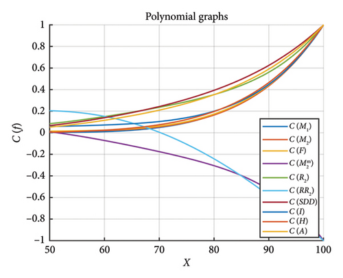
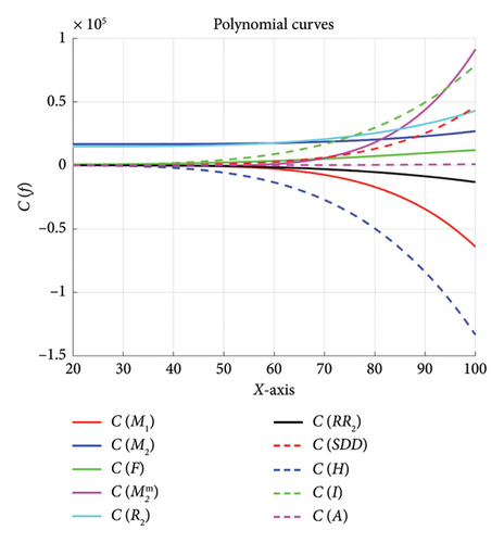
Example 3. Consider the first six values of p to obtain the following polynomials, where Figure 2 indicates their approximated curves.
- 1.
- 2.
- 3.
PT(F)(x) = 1.04762x5 − 176.2857x4 + 11360.5714x3 − 343628.1905x2 + 5256857.1429x − 30629714.2857
- 4.
- 5.
- 6.
- 7.
PT(SDD)(x) = 0.003968x5 − 0.952381x4 + 92.063492x3 − 3749.142857x2 + 67478.730159x − 443001.142857
- 8.
PT(H)(x) = 0.000035x5 − 0.006548x4 + 0.497421x3 − 17.911806x2 + 290.565728x − 1761.263587
- 9.
PT(I)(x) = 0.000065x5 − 0.012659x4 + 0.944373x3 − 32.968503x2 + 584.373185x − 2933.235597
- 10.
PT(A)(x) = 1.1244 × 10−5x5 − 2.5708 × 10−3x4 + 2.3489 × 10−1x3 − 9.0735x2 + 147.978x − 819.352
- •
: Coefficients generate higher order polynomials that record complex fluctuations, and the balance of positive and negative coefficients can exhibit oscillation behavior.
- •
: Indicate a more detailed or delicate pattern and larger coefficients suggest steeper curves or greater effects from higher terms.
- •
PT(F)(x): A minor rise in higher order coefficient relative to may imply refinement or alternative formulation.
- •
: Polynomial has small coefficients, indicating less significant deviations, and it could refer to a standardized or regularized version of .
- •
These polynomials can serve as regression models for data sets of various complexity.
- •
They could be produced from optimization procedures focused on certain loss or objective functions.
- •
have greater coefficients for the higher terms, indicating that these polynomials represent steeper, more dynamic systems.
- •
show lower coefficients for higher terms, indicating weaker or greater local variability.
- •
Higher magnitude coefficients (e.g., 404717.5238x, 705882352.9412x) indicate that these polynomials are more sensitive to input changes.
- •
Coefficients like 10−9, 10−3 indicate that these are intended for accurate, localized forecasts.
- •
Polynomials with large x5, x4, x3 coefficients are likely to produce sharper oscillations.
Table 4 provides the characteristics and likely use cases of the polynomials.
| Polynomial | Characteristics | Likely use case |
|---|---|---|
| Large coefficients; steep gradients. | Complex systems with rapid variations or higher order dynamics. | |
| Similar to but more pronounced coefficients for higher order terms. | More detailed modeling of large-scale trends. | |
| PT(F)(x) | Follows , refined for feature F. | Captures features in highly dynamic systems. |
| Small coefficients; smooth curve. | Regularized or normalized model. | |
| Extremely large coefficients; dramatic variations. | Systems with extreme values or highly sensitive predictions. | |
| Negligible higher order coefficients; focuses on lower order terms. | Residual corrections or fine-tuning models. | |
| PT(SDD)(x) | Intermediate coefficients; balanced between precision and large-scale behavior. | Variability modeling, potentially related to uncertainty estimation. |
| PT(H)(x) | Small coefficients; low sensitivity to higher order variations. | Stable feature modeling (e.g., height). |
| PT(I)(x) | Slightly larger coefficients compared to PT(H)(x). | Similar to PT(H)(x), with slightly more complexity. |
| PT(A)(x) | Moderate coefficients, low-order terms dominate. | Averaging or aggregated effects. |
Theorem 8. Let and p be any FWIPQ of the class Ξ and a positive integer, respectively, where λ = 2(2p + 1). Then, following are the topological sequences associated with :
- 1.
T(M1) = 27λ3 − 54λ2 + 39λ − 10
- 2.
T(M2) = (81/2)λ4 − (243/2)λ3 + (297/2)λ2 − (177/2)λ + 21
- 3.
T(F) = 81λ4 − 243λ3 + 297λ2 − 171λ + 38
- 4.
- 5.
T(R2) = (729/2)λ6 − (3645/2)λ5 + 4050λ4 − 5103λ3 + (7569/2)λ2 − (3069/2)λ + 261
- 6.
T(RR2) = (81λ4 − 189λ3 + 90λ2 + 48λ − 32/1458λ6 − 7776λ5 + 17172λ4 − 20088λ3 + 13122λ2 − 4536λ + 648)
- 7.
T(SDD) = (81λ4 − 216λ3 + 207λ2 − 78λ + 8/9λ2 − 15λ + 6)
- 8.
T(H) = (54λ3 − 99λ2 + 45λ − 2/36λ2 − 66λ + 30)
- 9.
T(I) = (162λ4 − 459λ3 + 504λ2 − 261λ + 54/24λ − 20)
- 10.
T(A) = (ψ9(λ)/ψ10(λ))
Proof 6. We have the partitions of Θ and Υ as follows:
These partitions and equation (5) provide the following first Zagreb topological sequence as:
With the help of equation (6), second Zagreb topological sequence can be calculated as follows:
Equation (7) can be used to find the forgotten topological sequence as follows:
Following is the calculation of second modified Zagreb topological sequence by equation (4):
Equation (5) gives the generalized Randić topological sequence at χ = 2 as follows:
Following lines show, with the help of equation (6), the inverse Randić topological sequence at χ = 2:
Following is the computation of symmetric degree topological sequence by equation (7):
With the help of equation (8), harmonic topological sequence can be calculated as follows:
Equation (9) can be used to find the inverse sum indeg topological sequence as follows:
Following lines show, with the help of equation (10), the augmented Zagreb topological sequence:
Coefficients of ψ9(λ) and ψ10(λ) can be seen in Table 5. Using the same vertex and edge partitions, we can write the other results. It completes the proof.
| Power of λ | ψ9(λ) | ψ10(λ) | ψ11(λ) | ψ12(λ) |
|---|---|---|---|---|
| λ11 | 1,417,176 | — | 472,392 | — |
| λ10 | −14,880,348 | — | −3385,476 | — |
| λ9 | 71,528,022 | — | 11,114,334 | — |
| λ8 | −208,488,897 | — | −22,152,123 | — |
| λ7 | 410,642,055 | — | 29,855,466 | — |
| λ6 | −574,949,907 | 93,312 | −28,571,697 | 31,104 |
| λ5 | 584,199,459 | −699,840 | 19,764,972 | −171,072 |
| λ4 | −430,326,189 | 2,185,056 | −9841,068 | 391,392 |
| λ3 | 224,667,621 | −3635,280 | 3,438,000 | −476,784 |
| λ2 | −78,923,565 | 3,398,976 | −798,288 | 326,160 |
| λ1 | 16,730,307 | −1693,440 | 110,336 | −118,800 |
| λ0 | −1615,734 | 351,232 | −6848 | 18,000 |
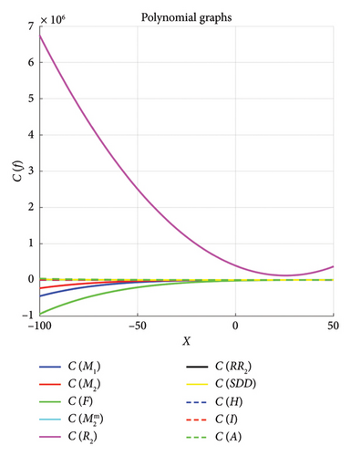
Example 4. Figure 3 shows the approximated curves of the following polynomials when λ = 6, 10, 14, 18, 22, 26.
- 1.
- 2.
- 3.
PT(F)(x) = 2.378 × 10−6x5 − 0.001527x4 + 0.32568x3 − 29.5273x2 + 1241.526x − 17765.779
- 4.
- 5.
- 6.
- 7.
PT(SDD)(x) = −1.249 × 10−7x5 + 0.000078x4 − 0.004303x3 + 0.08997x2 − 0.6047x + 113.675
- 8.
PT(H)(x) = −1.672 × 10−8x5 + 4.859 × 10−6x4 − 5.936 × 10−4x3 + 0.034227x2 − 0.634726x + 29.493637
- 9.
PT(I)(x) = −1.251 × 10−7x5 + 0.000027x4 − 0.002016x3 + 0.086132x2 − 1.5677x + 1033.116
- 10.
PT(A)(x) = −2.783 × 10−7x5 + 2.571 × 10−4x4 − 0.008039x3 + 0.10459x2 − 2.3656x + 1072.457
- •
The balance of coefficients in the terms shows the model’s resilience and generalizability. Small coefficients typically reflect regularity.
- •
During training, these coefficients are optimized to reduce error, making them more crucial to the model’s success.
- •
The coefficients can be used to evaluate the key impacts and relationships modeled.
- •
PT(A)(x): The quadratic term has the most significant effect and may reveal medium-term trends.
- •
PT(I)(x): The addition of big constant terms constrains the model, potentially leading to more broad predictions.
- •
: All coefficients are extremely small, implying that they are smoothed out or simulated in the noise.
- •
PT(F)(x): The negative constant term −17765.779 stops the polynomial from taking all possible values, potentially affecting specific data points.
- •
: Strong quadratic and linear terms characterizing local or immediate patterns predominate.
Role of polynomials in ML can be seen in Table 6.
| Polynomial | Characteristics | Most likely use case |
|---|---|---|
| Higher order terms (x5, x4) have smaller contributions. Dominated by quadratic (x2) and linear (x) terms. Alternating positive and negative coefficients balance the model. | Models general trends or behaviors in metric M1. Useful for analyzing nonlinear patterns in data. | |
| Similar to but with smaller coefficients for higher order terms. Strong influence from quadratic and linear terms. | Captures trends in a related or derivative metric M2. May focus on local or immediate patterns. | |
| PT(F)(x) | Significant quadratic and linear coefficients dominate, while higher order terms are less influential. Large negative constant offsets the function. | Likely represents a complex or aggregated feature F. May emphasize specific dominant patterns in data. |
| All coefficients are small. Dominated by lower order terms (x2, x). | Models adjustments or residuals of M2, possibly capturing fine-tuned corrections. | |
| Large quadratic term dominates, with a very high constant term reflecting baseline effects. | Likely models a robustness metric or R2 statistic, focusing on variance explained by the quadratic relationship. | |
| Smaller coefficients than , with a tempered quadratic term. Contributions from higher order terms are minimal. | Represents an adjusted robustness metric, focusing on refined or smoothed variability. | |
| PT(SDD)(x) | Moderate contributions from quadratic and cubic terms, with a high constant term. | Likely models standard deviation dynamics (SDD), capturing medium-term fluctuations in variability. |
| PT(H)(x) | Very small coefficients for higher order terms. Lower order terms dominate the relationship. | Represents an entropy or randomness metric H, likely focusing on simpler relationships. |
| PT(I)(x) | Strong quadratic and linear terms dominate. Large constant term offsets the model. | Models information I, possibly mutual information or related metrics. Reflects significant clear relationships. |
| PT(A)(x) | Moderate contributions from all terms, with significant influence from the quadratic term. | Likely represents an aggregate metric A, capturing balanced medium-term trends. |
Theorem 9. Let λ > 1 and be the odd positive integer and quasi-inverse graph of an element of the class Ξ, respectively. Then, following are the degree-based sequences:
- 1.
T(M1) = 27λ3 − 36λ2 + 18λ − 3
- 2.
T(M2) = (81/2)λ4 − 81λ3 + (135/2)λ2 − 27λ + 4
- 3.
T(F) = 81λ4 − 162λ3 + 135λ2 − 51λ + 7
- 4.
- 5.
T(R2) = (729/2)λ6 − 1215λ5 + (3645/2)λ4 − 1539λ3 + 747λ2 − 192λ + 20
- 6.
T(RR2) = (729λ6 − 1944λ5 + 1782λ4 − 486λ3 − 189λ2 + 132λ − 20/13122λ8 − 61236λ7 + 123930λ6 − 141912λ5 + 100440λ4 − 44928λ3 + 12384λ2 − 1920λ + 128)
- 7.
T(SDD) = (81λ4 − 135λ3 + 81λ2 − 18λ + 1/9λ2 − 9λ + 2)
- 8.
T(H) = (54λ3 − 63λ2 + 18λ − 1/36λ2 − 42λ + 12)
- 9.
T(I) = (486λ5 − 1215λ4 + 1242λ3 − 657λ2 + 180λ − 20/72λ2 − 84λ + 24)
- 10.
T(A) = (ψ11(λ)/ψ12(λ))
Proof 7. Both sets Θ and Υ can be partitioned as follows:
These partitions and equation (5) provide the following first Zagreb topological sequence as:
With the help of equation (6), second Zagreb topological sequence can be calculated as follows:
Equation (7) can be used to find the forgotten topological sequence as follows:
Following is the calculation of second modified Zagreb topological sequence by equation (4):
Equation (5) gives the generalized Randić topological sequence at χ = 2 as follows:
Following lines show, with the help of equation (6), the inverse Randi ć topological sequence at χ = 2:
Following is the computation of symmetric degree topological sequence by equation (7):
With the help of equation (8), harmonic topological sequence can be calculated as follows:
Equation (9) can be used to find the inverse sum indeg topological sequence as follows:
Following lines show, with the help of equation (10), the augmented Zagreb topological sequence:
Coefficients of ψ11(λ) and ψ12(λ) can be seen in Table 5. Other results can be obtained similarly. It completes the proof.
Example 5.
- a.
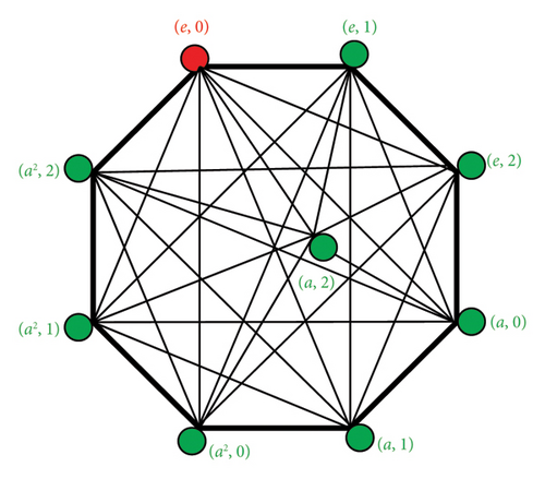
For the nine-order FWIPQ , (Figure 4) shows the nonisomorphic quasi-inverse graph.
- b.
When λ = 3, 5, 7, 9, 11, 13, Figure 5 indicates the approximated curves C(f) of the following fifth-degree polynomials:
- 1.
- 2.
- 3.
PT(F)(x) = −4.889 × 10−6x5 + 1.231 × 10−3x4 − 0.1153x3 + 6.927x2 − 186.67x + 2472.14
- 4.
- 5.
- 6.
- 7.
PT(SDD)(x) = 1.242 × 10−5x5 − 0.001356x4 + 0.07394x3 − 1.8596x2 + 24.881x − 124.04
- 8.
PT(H)(x) = 2.245 × 10−6x5 − 2.539 × 10−3x4 + 0.1289x3 − 3.548x2 + 49.343x − 232.52
- 9.
PT(I)(x) = −1.135 × 10−6x5 + 1.865 × 10−3x4 − 0.1641x3 + 8.4127x2 − 176.523x + 1260.2
- 10.
PT(A)(x) = −7.934 × 10−9x5 + 2.204 × 10−5x4 − 0.002366x3 + 0.1427x2 − 3.3632x + 38.736
- 1.
-
These polynomial coefficients are used in ML to provide weights for feature interactions of varying complexity.
- •
Polynomials such as , and PT(F)(x) include terms x4 and x5, indicating that they represent complex processes with limited effects.
- •
Polynomials like and PT(SDD)(x) contribute considerable monomials 3.409 × 10−5x5 and 1.242 × 10−5x5, respectively, making them ideal for fine-grained adjustments or sensitivity analysis.
- •
and use quadratic terms to explain variance and assess robustness.
- •
PT(I)(x) emphasizes mutual information or interdependence within the models through deep intimate relationships.
- •
, and PT(A)(x) are well-suited for capturing general trends or scaling features across datasets.
- •
-
For the odd positive integer λ, Table 7 gives the implications of polynomials in ML.
- c.
Polynomial Validation
-
Using the aforementioned feature engineering and ML model evaluation approach, we can validate the role of these polynomial coefficients.
-
Approach:
- •
Calculate polynomial values based on provided x values.
- •
Apply them as input features for classification and regression models.
- •
Measure effectiveness to models without polynomial features.
- •
-
Steps:
- •
Determine the PT(f)(x) values for each polynomial and apply them as new input features.
- •
Train models that involve Random Forest, SVM, and neural networks.
- •
Examine accuracy, MSE, and value pairs.
- •
| Polynomial | Characteristics | Most likely use case |
|---|---|---|
| Moderate higher order contributions (x4, x5), strong quadratic and cubic terms. Captures general trends in data. | Trend identification in metrics or feature scaling. | |
| Small x5, moderate x4. Dominance of x2 and x3. Captures localized patterns. | Capturing variations or behavior of M2 for extended trend analysis. | |
| PT(F)(x) | Moderate higher order terms, strong x2 and x3. High constant term indicates baseline offset. | Feature aggregation and representation of derived metrics. |
| Significant x5, strong x4, and dominant x3. Captures fine-grained corrections. | Residual modeling and correction for M2. | |
| Small x5, moderate x4. Strong quadratic and cubic terms. | Robustness analysis, variance explanation in regression models. | |
| Negligible x5, strong x3, and x2 terms. | Refined robustness metric for residual noise analysis. | |
| PT(SDD)(x) | Moderate x5, x4, strong quadratic, and cubic terms. High variability representation. | Capturing variability and periodic dynamics, e.g., time-series data. |
| PT(H)(x) | Small x5, moderate x4. Focused on x2 and x3 for complexity patterns. | Entropy analysis for randomness or structural complexity in datasets. |
| PT(I)(x) | Negligible x5, strong x4, and x3. High constant term reflects baseline. | Mutual information or feature interdependence modeling. |
| PT(A)(x) | Negligible x5, x4. Strong x2 and x3 terms. Captures balanced patterns. | Aggregate metric representation for overall trend analysis. |
Theorem 10. Let be any quasi-inverse graph of FWIPQ with positive integers p and λ > 1. Then following are the M-polynomials of the integral domain :
- a.
when λ = 4p
- b.
when λ = 2(2p + 1)
- c.
when λ is an odd integer.
Proof 8. These polynomials can be obtained, respectively, using partitions provided in Theorems 7, 8, and 9.
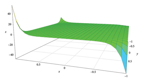
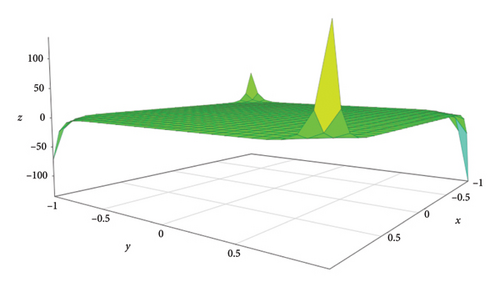
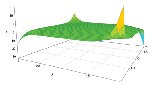
Example 6. 4x10y10 + 32x9y10 + 20x9y9, 32x15y16 + 104x15y15, and 8x7y8 + 24x7y7 are the M-polynomials of the quasi-inverse graphs , , and and their corresponding 3D geometrical representations can be seen in Figures 6, 7, and 8, respectively.
6. Conclusion and Future Directions
This study used polynomials as a foundation tool to analyze complex relationships between topological sequences T(f) and quasi-inverse graphs of finite FWIPQs. We developed and analyzed these graphs to give a framework for geometrically describing the algebraic features of FWIPQs. Connecting polynomials PT(f)(x) serve as a bridge between algebraic structures and topological configurations, allowing for extensive exploration of their interactions.
Furthermore, ML may be used to detect patterns and estimate the characteristics of these topological sequences. This novel approach confirmed the efficacy of ML in algebraic combination contexts and provided fresh insights into the structural dynamics of FWIPQs. The results demonstrate that it is feasible to effectively combine algebraic approaches, graph theory, and computational methods to tackle modern complicated mathematical problems.
Further studies might broaden the methods outlined in this paper to other algebraic structures, such as alternative quasigroups, Moufang quasigroups, and more classes of quasigroups when λ ≠ 4p and λ ≠ 2(2p + 1). This could assist them in finding novel connections between their inverted graphs. Analyzing high-dimensional graph representations and constructing topological invariants and associated polynomials are promising approaches. Advanced ML approaches, such as deep learning and generative models, can help improve prediction and inheritance distribution in algebraic systems. Additionally, applications in cryptography, specifically utilizing the algebraic and topological difficulty of FWIPQs for secure encryption, are a desirable extension. This work’s effects can be multiplied by establishing an efficient algorithm for large-scale calculations. Likewise, interconnected research in network theory, biology, and quantum computation may expand its influence. Together, these instructions seek to cover algebra, topology, and a variety of numerical approaches in depth.
Conflicts of Interest
The authors declare no conflicts of interest.
Funding
The authors extend their appreciation to the Deanship of Scientific Research at Northern Border University, Arar, KSA, for funding this research work through the project number “NBU-FFR-2025-1102-07.”
Acknowledgments
The authors extend their appreciation to the Deanship of Scientific Research at Northern Border University, Arar, KSA, for funding this research work through the project number “NBU-FFR-2025-1102-07.”
Open Research
Data Availability Statement
Data sharing is not applicable to this article as no datasets were generated or analyzed during the current study.


