This present article was written to analyze the variability of the diurnal profiles of the critical foF2 frequencies in the light of solar radiation based on in situ measurements of the ionosonde stations of Dakar (latitude 14.8° N, longitude 342.6° E) and Ouagadougou (latitude 12.5° N, longitude 358.5° E), respectively, for Sunspot Cycles 21 and 22. The objective being to deduce interpretations in terms of propensity to occur on the five profiles B, M, R, D, and P referenced to occurrence between the latitudes of 20° N and 20° S. Thus, on the analyses of conjunctions in phases or in phase shift observed in the variation of the sunspot cycle (VSC) and monthly foF2 frequencies (MFVs), we will note the following: (1) during periods of geomagnetic calm, (a) a propensity for the formation of the R profile during the growth phases of the solar cycle and during the periods from the solstices to the equinoxes and this is due to the conjunction in the growth–growth phase between VSC and MFV; (b) a propensity for the formation of the M profile during the waning phases of the solar cycle and during the periods from the equinoxes to the solstices and this is due to the conjunction in the waning–decaying phase between VSC and MFV; (c) a propensity for the formation of profiles B, D, and P on the one hand during the growth phases of the solar cycle and during the periods from the equinoxes to the solstices and on the other hand during the waning phases of the solar cycle and during the periods from the solstices to the equinoxes and all these are due to the nonconjunction in the phase between VSC and MFV. It therefore appears that out of the 16 possible propensities for profile formations, the R and M profiles are each counted for 12.5%. Profiles B, P, and D each counted 25%. (2) During periods of geomagnetic disturbances, notably by SFEs, CMEs, or ionization losses, a profile can transform into one or other of the other four profiles. Finally, as an importance or application of this study, we note that (a) foF2 contributes more to the good knowledge of the ionosphere; (b) using the diurnal profiles of foF2, we could a priori identify periods of lulls in radio or satellite transmission; (c) by induction, we could count the solar flares during the day; and (d) the proposed mathematical model is a basic tool for analyzing foF2 variability.

1. Introduction

The critical foF2 frequencies present in their diurnal variabilities five types of profiles referenced and named B, M, R, P, and D [1] and which are analyzed in terms of equatorial electrojets (EEJ) [2, 3] and counter-electrojets (CEJ) [4]. Although these interpretations to date are entirely plausible for many authors, one wonders if we could not also refer to other interpretations. Could not another alternative explanation, notably by the rays of the Sun, as this article claims, be completely satisfactory? A sufficiently conceivable alternative, especially since: (a) On the one hand, it is unanimously recognized and accepted by the scientific community that solar radiation is the main factor in ionization of the sublayers of the ionosphere, namely, the F2 sublayer, and (b) on the other hand, this reflection follows our previous work [5, 6] where using a proposed formula for the power of solar radiation, we could also carry out an analysis through a mathematical model. So, to do this, after having indicated the data, the equipment, and the methodology used, we will strive in the Results section and Discussion section to convince on the profiles named B, M, R, P, and D in the light of solar radiation.

2. Data and Materials

The data used are in situ measurements of the critical foF2 frequencies of Solar Cycle 21 at the Dakar ionosonde station (latitude 14.8° N, longitude 342.6° E) and of Cycle 22 at the Ouagadougou ionosonde station (latitude 12.5° N, longitude 358.5° E). Excel 2010 is used for data processing (compilation, graphing). These stations were chosen due to the availability of data from in situ measurements.

3. Methodology

The analysis of the diurnal variability of critical foF2 frequencies in the light of solar radiation started from the observation of the monthly variability of foF2 and that of the sunspot cycle (SC) which depending on the periods (solstices to equinoxes or from equinoxes to solstices) could be in phase conjunction or not. Also, this analysis is also part of the observation of the good correlation existing between the variations of the critical foF2 frequencies and of the F10.7 cm flux of solar radiation and the SC. Thus, the monthly variability curves of foF2 (Ouagadougou and Dakar stations) were obtained by carrying out a statistical compilation of data from in situ measurements. This compilation will be carried out using the Excel 2010 Pivot Table while taking into account the periods of the different phases of the SC. These different phases are phase minimum, rising phase, phase maximum, and falling phase. The periods of the different phases were established according to a spot index or Wolf R index which makes it possible to characterize this type of activity. This Wolf index is given by the following relation:

()

where R_z designates the relative number of spots or Wolf number, g designates the number of groups of spots, f the number of spots, and k a corrective or normalization term which takes into account the sensitivity of the measuring devices and the observer. Thus, from the classification of the phases of the SC according to the number R_z and according to [7], we obtain Table 1 of the phases of the SCs 21 and 22 extracted from the thesis work of [8].

Table 1. Distribution of years of measurements by the phase of the solar cycle [8].

Phases	Number of sunspots	Periods of SC21	Periods of SC22
Minimum	R_Z < 20	1975–1976	1985–1986
Ascending	20 ≤ R_Z ≤ 100	1977–1978	1987
Maximum	R_Z > 100	1979–1982	1988–1991
Descending	100 ≥ R_Z ≥ 20	1983–1984	1992–1994

After that, postulates will be formulated. (a) The phase conjunction observed both during the phases of the solar cycle and the monthly variability of foF2 would explain the propensity for the formation of the reversed R profiles in the growth phases and morning peak M in the decay phases. (b) The phase shift conjunction observed would explain the propensity for the formation of noon bite out B profiles (where the lower part or “hollow” at noon testifies to the vertical rise of the plasma, also called the signature of with the electric field vector of the plasma and the Earth’s magnetic field vector), dome D, and plateau P. (c) The transformations of the M, R, B, D, and P profiles can be plausibly explained by ionization enhancements from solar flare effects (SFE), coronal mass ejections (CME), and solar winds, as well as ionization losses from recombinations and delocalizations.

4. Results and Discussion

4.1. Theory of the EEJ and CEJ

The diurnal variations of the critical foF2 frequencies observed between the latitudes of 20° N and 20° S can be presented in the form of five types of profiles denoted M, R, B, D, and P [1]. As shown in Figure 1, (a) profile B will be called noon bite out, (b) profile M called morning peak, (c) the R profile called reversed, (d) profile D called dome, and finally (e) profile P called plateau.

Details are in the caption following the image — **Figure 1**
Open in figure viewer PowerPoint

Five foF2 profiles [1]. Abscissa axis: hours of the day. Y axis: foF2 (MHz).

The interpretation or analysis of these different diurnal variability profiles is made by certain authors in the light of EEJ and CEJ which testify to the geomagnetic activity generated during the day by ionospheric currents. The EEJ for its part is an ionospheric electric current circulating from West to East with a field vector () centered on a 600-km belt on the geomagnetic equator as shown in Figure 2. The electrojet circulating from West to East () was first named by [9].

The vector product of such a field vector (

) with the magnetic field vector (

) which is horizontal to the Earth’s equator and oriented towards the North causes an increase in ionization at the speed (

). This rise is also called vertical drift and thus contributes through the F2 sublayer to reinforce the ionization in this part as shown in Figure 3. To this end, we note that

()

The CEJs will be explained [4] by the decrease in the horizontal component of the magnetic field which is oriented towards the South. Thus, a reverse movement will then be observed.

Thus, according to [11], the following interpretations follow: (a) Profile B testifies to the presence of an electrojet in the morning of the same intensity as the CEJ observed in the evening; (b) the M profile, the presence of a strong electrojet in the morning and the absence or presence of a weak CEJ in the evening; (c) the R profile of a weak electrojet in the morning and a strong CEJ in the evening; (d) the P profile of the presence of an average electrojet during the day; and (e) finally, profile D, the absence of electrojet and CEJ during the day

The EEJ by the fountain effect theory as shown in Figure 3 also provides an explanation for the equatorial ionization anomaly (EIA). However, in order not to make this present article complex, the problem of the EIA under the spectrum of solar radiation will be addressed later.

As this article is intended, we can also find an explanation in terms of solar radiation for the fact that (a) on the one hand, the power of solar radiation as well as the critical frequencies of foF2 is correlated to the SC like the one shown in Figure 4 [12] and (b) on the other hand, this power would vary depending on the Earth–Sun distance and the angles of incidence [5, 6] plausibly explaining the observed monthly variability of critical foF2 frequencies.

4.2. Analysis Tools Based on Solar Radiation

The monthly variability of foF2, the SC and the continuity equation through the factors that can influence the production and ionization losses are the main tools for analyzing the diurnal profiles of foF2 in the light of solar radiation.

Indeed, and for example, the observation in Figure 5 of the monthly variability of the critical foF2 frequencies of the Solar Cycles 22 of the ionosonde station of Ouagadougou and 21 of Dakar shows the following: high ionization densities of the F2 sublayer at equinoxes and minima in the ionization density at the solstices, although with asymmetries. An asymmetry of ionization peaks at the equinoxes and solstices: (a) asymmetry at the equinoxes called equinoctial asymmetry. This is due to the fact that the power allocated to the Earth–Sun distance decreases from the winter solstice to the spring equinox. On the other hand, it grows from the summer solstice to the autumn equinox [5, 6]; (b) asymmetry at the solstices called winter or seasonal anomaly. This is due to the fact that the power allocated to the Earth–Sun distance and that allocated to the angles of incidence decrease from the spring equinox to the summer solstice. On the other hand, the power allocated to the Earth–Sun distance increases from the autumn equinox to the winter solstice and that allocated to the angles of incidence decreases [5, 6]; (c) the disparities observed between the equinoxes and the solstices called semiannual or semiannual anomaly. This is due to the fact that the power imparted to the angles of incidence is always increasing from the solstices to the equinoxes. On the other hand, this same power imparted to the angles of incidence always decreases from the equinoxes to the solstices [5, 6].

Thus, it appears that the power of solar radiation, the main ionization factor, will be as follows: (a) increasing from the solstices to the equinoxes, for this purpose, from the winter solstice to the spring equinox (December 21–March 21) and from the summer solstice to the autumn equinox (June 21–September 23), and (b) decreasing from the equinoxes to the solstices, for this purpose, from the spring equinox to the summer solstice (March 21–June 21) and from the autumn equinox to the winter solstice (September 23–December 21).

This characteristic in the monthly variability will also a priori be observed in the diurnal variability of the critical foF2 frequencies as shown in Figure 6. Indeed, during the day, two maximum peaks and two minimum peaks will be observed in the ionization density, also with asymmetries. The maximum peaks will be observed, one in midday in the morning around 9 a.m.–10 a.m. “spring equinox” and the other in the afternoon in the evening around 4 p.m.–6 p.m. “autumn equinox.” As for the peaks of the minimums, one will be observed at dawn around 5 a.m. “start of winter solstice,” at noon 12 p.m. “summer solstice,” and the other at dusk 6 p.m.–7 p.m. “end of winter solstice” with an asymmetry almost always in favor of the peak of the midday minimum.

Such profiles will not be observed all the time because we could observe the formation of a single maxima peak or even the absence of formation of maxima peaks as evidenced by the five types of profiles M, R, B, D, and P of diurnal variability of critical foF2 frequencies shown in Figure 1.

Also, this analysis of the interpretation of the diurnal profiles of the critical foF2 frequencies would also take into account the SC as shown in Figure 7 (National Oceanic and Atmospheric Administration (NOAA)) of Cycles 20, 21, and 22. On these different curves of almost symmetrical variability, we will mainly distinguish an ascending phase and a descending phase. The ascending phase (in the broader sense) goes from the beginning of the cycle to the peak of the maximum phase where the power of solar radiation increases more and more. The descending phase (in the broader sense) goes from the maximum peak to the end of the cycle where the power of solar radiation decreases more and more.

So, for this purpose, if it only depended on the SC, (a) for the days during a year of the ascending phase, the ionization would tend to be maximum in the afternoons (autumn equinox). This is true due to the contribution of additional power and therefore increasingly increasing ionization from morning to evening to the radiation by sunspots. This is all the more noticeable in the variation monthly or seasonal foF2 during the ascending phase where we observe an equinoctial asymmetry in favor of the autumn peak as shown in the example of Figure 8 [5, 6].

(b) For days during a year of the descending phase, ionization would tend to be maximum during the mornings (spring equinox). This is true due to the provision of additional power and therefore increasingly decreasing ionization from morning to evening to the radiation by sunspots. This is all the more noticeable because in the monthly or seasonal variation of foF2 during the descending phase, we observe an equinoctial asymmetry in favor of the spring peak as shown in Figure 9 (Ouagadougou C22).

Finally, this analysis of the diurnal foF2 profiles would take from the continuity equation (Equation (3)) through the duality of factors on the one hand which influence the production of ionization such as CMEs, solar flares by these SFEs and on the other hand ionization losses. The continuity equation known as the equation of [13] is as follows:

()

Thus, it translates that the variability in the temporal density of an electric or nonelectric N particle is its production q(t) deducted from the losses generated, among other things, by recombinations l(t) and transport mechanisms with the velocity vector of the particle.

SFEs as shown in Figure 10 (National Aeronautics and Space Administration (NASA)) are energetic “or splashing” luminosity which accompany solar flares and can occur in the mornings or afternoons or throughout the daytime.

These SFEs are perceptible by their signature or magnetic disturbance which appears on the magnetograms in the form of a hook or magnetic peak as shown in Figure 11 [14].

These SFEs provide additional power to the power of solar radiation which will therefore induce more ionization depending on the class (A or B or C or M or X) of these solar flares. From one intensity class lower to the next, the intensity of the radiation is multiplied by a factor of 10 and within the same class, a number ranging from 1 to 9.9 is used to specify the degree of the radiation. Thus, a Class M solar flare is more intense than a Class C flare and a Class C1.6 flare is less intense than a Class C7.4 flare.

The CMEs [15] for their part, as shown in Figure 12, are ejections of enormous quantities of plasma from the solar corona. CMEs cause geomagnetic storms due to their interaction with the Earth’s magnetosphere. These CMEs for some are due to the breakage of the dipolar magnetic field lines of the Sun and for others to the breakage of the unipolar magnetic field lines.

However, the action of SFEs is more instantaneous than that of CMEs or solar winds. Light or solar radiation takes less than 7 min from the Sun to the Earth while fast solar winds have a speed of 700 to 1000 km/s, therefore taking 2–3 days before reaching the Earth. Also taking into account the obliquity (11.43°) of the Earth, the action of the SFEs will be instantly felt more at the level of the Tropics of Cancer (23°26 ^′ N) or Capricorn (23°26 ^′ S) at the equator while the CMEs much more at the level of the North and South poles of the Earth as evidenced by the northern and southern lights. The action of these different factors reinforcing ionization can be symbolized by P_SolarFlare(t) for latitudes from 20° N to 20° S. The ionization losses are symbolized by P_Loss(t).

All these result in fluctuations observed in the variability of the critical foF2 frequencies depending on the days as shown in Figure 13, thus highlighting the duality ΔP(t) between ionization losses P_Loss(t) and ionization enhancement P_SolarFlare(t) which boils down to the following equation [6]:

()

Then, (a) the observed periods of decrease in the daily variability of foF2 would mean that P_Loss(t) power was predominant over P_SolarFlare(t) and (b) the observed periods of increase in the daily variability of foF2 would mean that P_SolarFlare(t) power was predominant over P_Loss(t).

4.3. Interpretation in the Light of Solar Radiation

According to the position of the Earth in its progression around the Sun as shown in Figure 14, the year has been subdivided into four seasons which are winter which will be announced by the winter solstice on December 21, spring announced by the spring equinox on March 21, summer announced by the summer solstice on June 21, and finally autumn by the autumn equinox on September 23.

Thus, depending on the conjunction in the phase or out of phase between the phase of the SC and the monthly variability of foF2, we will note in this period the propensity for the formation of one of the five profiles.

4.3.1. R and M Profiles

1.
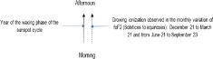
For a day during the growth phase of the solar cycle and from the solstices to the equinoxes, we will note a propensity for the formation of the reversed R profile. This is all the more true because there is a conjunction in the phase (growth–growth) between the SC and monthly foF2 variability.

Propensity for the formation of the reversed R profile

2.
On the other hand, for a day during the decay phase of the solar cycle and from the equinoxes to the solstices, we will note a propensity for the formation of the morning peak M profile. This is all the more true because there is a conjunction in the phase (decay–decay) between the SC and the monthly variability of foF2.

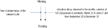
Propensity for the formation of the morning peak M profile

4.3.2. B, D, and P Profiles

1.
For 1 day during the growth phase of the solar cycle and from the equinoxes to the solstices
2.
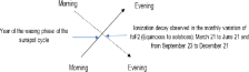
Also, for 1 day during the waning phase of the solar cycle and from the solstices to the equinoxes
3.
We will note in these periods a propensity for the formation of profiles noon bite out B, dome D, and plateau P. This is all the more true because there is a conjunction in phase shift (growth–decrease or decrease–growth) between the SC and the monthly variability of foF2. Thus, we will obtain the following illustrations:

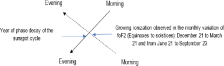
Propensity for the formation of the B, D, and P profiles

In short, we distinguish a total of 16 possible propensities for the formation of diurnal profiles of foF2, which are summarized well in Figure 15 in the Results section. Thus, in percentage terms, the propensity for the formation of profile B will be 25%, P 25%, and D 25% and profile M 12.5% and R 12.5%.

4.3.3. Profile Transformation Mechanisms

Although a certain period of the year corresponds to the propensity for the formation of a given profile, one could obtain instead another profile and this is due to the mechanisms of reinforcement of the ionization by the SFE symbolized by P_SolarFlare(t) or of losses of ionization symbolized as P_Loss(t).

The mechanisms for transforming profile M into R or into B or into D or into P are explained in the Results section in Table 2. Table 3 explains the mechanisms of transforming profile R into either M or into B or into D or either in P.

Table 2. M profile transformation mechanisms.

M to R	The R profile thus shows that the effect of reinforcing ionization by P_SFE(t) was very important at the evening peak. P_SFE(t) ≫ P_Loss(t)
M to B	Profile B thus showing that the P_SFE(t) effect was significant or medium at the evening peak. P_SFE(t) > P_Loss(t)
M to D	If during midday the loss of ionization by the preponderance of the transport mechanisms P_Loss(t) was very significant [P_SFE(t) ≪ P_Loss(t)] followed in the afternoon by the reinforcement by the SFE P_SFE(t) which is equally very important [P_SFE(t) ≫ P_Loss(t)], we will end up with the formation of profile D
M to P	If during midday the loss of ionization by the preponderance of the transport mechanisms was significant or medium [P_SFE(t) < P_Loss(t)] followed in the afternoon by the reinforcement by the SFE and all significant or medium [P_SFE(t) > P_Loss(t)], we will end up with the formation of profile P

Table 3. R profile transformation mechanisms.

R to M	The M profile thus shows that the effect of reinforcing ionization by P_SFE(t) was very important at morning peak. P_SFE(t) ≫ P_tp(t)
R to B	Profile B thus shows that the P_SFE(t) effect was significant or medium at morning peak. P_SFE(t) > P_tp(t)
R to D	If during midday the strengthening by the SFE was very significant [P_SFE(t) ≫ P_tp(t)], followed in the afternoon by the equally very important preponderance of transport mechanisms [P_SFE(t) ≪ P_tp(t)], it results in the formation of profile D
R to P	If during midday the strengthening by the SFE was significant or medium [P_SFE(t) > P_tp(t)], followed in the afternoon by the equally significant or medium preponderance of transport mechanisms [P_SFE(t) < P_tp(t)], it results in the formation of profile P

Finally, for profiles B, D, and P, we could explain the mechanisms in these terms. For 1 day during the growth phase of the solar cycle from the equinoxes to the solstices and for 1 day during the decline phase of the solar cycle and from the solstices to the equinoxes, the expected profile will be Type B.

If profile B is not observed and we observe (c) profile M, then both in the growth and decline phases, the effect P_Solarflare(t) was very important at the morning peak. (d) If during midday the loss of ionization by the preponderance of losses was very significant followed in the afternoons by the strengthening by the SFE or the equally very significant winds, we will end up with the formation of profile D. (e) Finally, if this preponderance was only significant or average, we will end up with the formation of the P profile.

4.4. Importance

The ionosphere is one of the layers of the atmosphere extending from 50 to 650 km or more. This ionospheric layer is a very important plasma due to its usefulness not only in telecommunications (radiocommunication or satellite communication) but also in space weather. Its perfect or in-depth knowledge is necessary and the critical frequencies foE, foD, foF1, and foF2 contribute to this effect. Thus, by knowing the diurnal profiles of foF2, we could on the one hand identify the periods or seasons where the “sky” appears “clearer or not” in terms of radiocommunication and GPS precision, for example. Also, by induction, we could become aware of many phenomena or activities of the Sun such as the SFEs and the CMEs which occur.

5. Mathematical Model

5.1. Components of Solar Radiation Power

At a given point in geographic coordinate space such as its latitude θ and its longitude φ, the power of the main solar radiation ionization factor presents a temporal variation P_s(t). This temporal variation takes place around the quasiconstants which are the component P_s(θ) latitudinal power and longitudinal power P_s(φ). We then note for this purpose that [6]

()

5.2. Temporal Variation of the Power of Solar Radiation

5.2.1. Own Power P₀(t)

The temporal variation of the power of the Sun has four components which are P₀(t), P_a(t), P_Solarflare(t) and P_Loss(t).

The component P₀(t) is called self-power, and it is this which varies according to the angles of incidence and the Earth–solar distance. It is given by the following formula [5, 6]:

()

The temporal variation of this power would allow on the one hand (a) to reproduce, if the weather is monthly, the half-yearly, winter, or seasonal anomalies and the equinoctial asymmetries and on the other hand (b) if the time is expressed in hours to reproduce the diurnal variation as shown in Figure 16 where we have oscillated for illustration P₀(t) around “10” average value corresponding to P_s(φ, θ).

Thus, the own power obtained highlights a diurnal profile presenting during the day (6 a.m.–7 p.m.) a morning peak at 10 a.m. of “10.5” lower than the evening peak observed at 6 p.m. of “12” although with a portion low called “trough” from 1 p.m. to 2 p.m. The gap or the difference between the value of the radiation power at the evening peak P_Pic(R) and the one in the morning P_Pic(M) would therefore make it possible to explain the propensity for the formation of profiles B, D, M, R, and P. The R terms in P_Pic(R) is used in reference to reversed and M in P_Pic(M) to that of morning. Thus, we will have an illustration for the initial gap observed through Figure 16:

()

5.2.2. Power P_a(t) Induced by Sunspot Effect

The component P_a(t) is that which reflects the additional power added to P₀(t) by sunspots. This effect is more remarkable in monthly terms but will be less so in daily terms given the relatively very short time. However, (a) its effect will contribute to increasing the initial gap in favor of the evening peak during the ascending phase.

()

(b) On the other hand, its effect during the descending phase will contribute to raising the morning peak more than that of the evening. Therefore, unless the morning peak is made higher than the evening peak, the gap between the two peaks will therefore decrease.

()

For example, suppose it is a descending phase and the effect of sunspots has increased the morning peak from “10.5” to “11.5,” thus a reduction of the initial deviation from “1.5” to “0.5”. To this end, we can observe a change in profile as shown in Figure 17.

5.2.3. Earth Position Effect P₀(t)

For the sunspot effect, it would also be necessary to take into account the position of the Earth during the year where the gap will fluctuate. Thus, in the ascending phase, we will observe an upward fluctuation from the solstices to the equinoxes taking into account the increase in natural power P₀(t) and this is for the benefit of the evening peak. In addition, a downward fluctuation is observed from the equinoxes to the solstices at the evening peak and would explain the decrease in the gap. However, the evening peak remains slightly higher than the morning peak. Also, a downward fluctuation from the equinoxes to the solstices gives the decrease in P₀(t). This is why we talk about the propensity for the formation of reversed profile “R” to the growth phase of the solar cycle if there is a conjunction in the phase with the monthly variation of foF2. There is a propensity for the formation of profiles B, D, and P if there is no phase or a nonconjunction.

For the descending phase, the same reasoning could apply. Thus, we will have a propensity for the formation of the morning peak M profile during the descending phase and periods from the equinoxes to the solstices. There is a propensity for the formation of profiles B, D, and P during the periods from the solstices to the equinoxes.

5.2.4. Ionization Enhancement Effect P_Solarflare(t) and Ionization Losses P_Loss(t)

The effects of ionization enhancement by solar flares or CMEs P_Solarflare(t) and loss P_Loss(t) by the different processes of recombination and delocalization have been largely explained above. To do this, let us simply take an example to illustrate. During the ascending phase and during the periods from the solstices to the equinoxes where we understand the formation of the reversed profile “R,” you can get another profile. In profile B shown in Figure 17, the solar flares at 10 a.m. or around 10 a.m. were of average or significant power. But in profile morning peak “M” as shown in Figure 18, the eruptions were very powerful.

5.3. Latitudinal and Longitudinal Variation of Solar Radiation Power

Less latitudinal power components P_s(θ) and longitudinal P_s(φ) are quasiconstants because if their variations in amplitude were very significant, they could impact P_s(t) going so far as to break its sinusoidal shape. However, if we take these fluctuations into account, they can justify the equatorial ionization anomalies with regard to the latitudinal power. The longitudinal power justifies the longitudinal profiles of foF2. Indeed, it emerged from the thesis presented by [16] on “Study of the Spatiotemporal Variability of the Equatorial Electrojet Based on Magnetic Data from the CHAMP Satellite” that “Seasonal variations of the longitudinal profiles of the equatorial electrojet (EEJ) were examined on the basis of all the magnetic measurements from the CHAMP satellite over the period 2001–2010. A total of 7537 passages of the satellite at noon across the magnetic equator was analyzed. This analysis showed that in average, the EEJ presents a longitudinal profile of four maxima located, respectively, around the longitudes 170° W, 80° W, 10° W and 100° E.” Figure 19 gives an illustration with ΔF_sat the magnetic field generated by the EEJ at the altitude of the satellite.

5.4. Importance

The proposed mathematical model made it possible to provide clarification on the diurnal variability of the critical foF2 frequencies, as in the previous analyses on the half-yearly or seasonal anomalies. The proposed equations are therefore basic analysis tools for the variability of critical foF2 frequencies and by extension other parameters.

6. Conclusion

At the end of this article relating to the analyses of the variability of the diurnal profiles of the critical foF2 frequencies in the light of solar radiation, it emerges as essential that (a) just as in the monthly variability of foF2, it appears at the equinox’s peaks of maxima in spring and autumn; it also appears in the diurnal variability of maximum peaks observed in the morning and evening. (b) Just as in the monthly variability of foF2, peaks of minima appear at the solstices in winter and summer; it also appears in the diurnal variability of the minimum peaks observed at dawn and dusk. (c) The more or less significant preponderance of one of the peaks over the other by the ionization reinforcements or even the ionization losses will lead to the formation of either type M or type R or type B profiles. (d) If during midday the strengthening by the SFE or the winds was very significant, followed in the afternoon by the equally very significant preponderance of ionization losses or conversely the losses in the morning and the reinforcement in the evening, it resulted in the formation of profile D. (e) Finally, if this preponderance was only significant or average, we will end up with the formation of profile P. It emerges in percentage terms that the propensity for the formation of profiles B will be 25%, P 25%, and D 25% and profiles M 12.5% and R 12.5%. The mathematical model proposed through the equations made it possible to provide substantial clarifications to the analysis. Finally, knowledge of variability diurnal critical foF2 frequencies contributes to knowledge of the ionosphere and further improves weather forecasting.

7. Recommendation

As a recommendation after the analysis of the diurnal profiles of foF2, we propose to analyze the phenomenon of EIA under the spectrum of solar radiation and also to reflect on the impact of the solar spectrum in the longitudinal variability of the critical foF2 frequencies or the total electron content (TEC).

Conflicts of Interest

The authors declare no conflicts of interest.

Funding

We did not receive funding for this manuscript. The financing was under own funds.

Acknowledgments

The authors would like to thank all the material or immaterial contributions, provision of resources, or others which contributed on the one hand to the writing of the article and on the other hand to the submission and acceptance of the article.

Open Research

Data Availability Statement

The data of the in situ measurements were made available to us by the National School of Telecommunications of Brittany and Europe Africa Ionospheric Reference Group.

References

1 Faynot J. M. and Vila P., F region at the magnetic equator, Annales Geophysicae. (1979) 35, 1–9.
Google Scholar
2 Reddy C. A., W. H. Campbell, The equatorial electrojet, Quiet Daily Geomagnetic Fields, 1989, Birkhäuser Basel, Basel, 485–508, https://doi.org/10.1007/978-3-0348-9280-3_11.
10.1007/978-3-0348-9280-3_11
Google Scholar
3 Untiedt J., A model of the equatorial electrojet involving meridional currents, Journal of Geophysical Research. (1967) 72, no. 23, 5799–5810, https://doi.org/10.1029/JZ072i023p05799.
10.1029/JZ072i023p05799
Web of Science® Google Scholar
4 Gouin P. and Mayaud P. N., A propos de l’existence possible d’un contre electrojet aux latitudes magnétiques équatoriales, Annales de Geophysique. (1967) 23, 41–47.
Web of Science® Google Scholar
5 Abdoul-Kader S., Allain G. D., and Salfo K., Contribution to the explanation of the semi-annual anomaly observed in the intertropical zone using the critical frequencies fof2 extracted during the sunspot cycles 20, 21 and 22 at the Ouagadougou station, International Journal of Advanced Research (IJAR). (2023) 11, no. 2, 412–417, https://doi.org/10.21474/IJAR01/16266.
10.21474/IJAR01/16266
Google Scholar
6 Abdoul-kader S., Allain G. D., and Aristide G., New analysis of the seasonal variation of the critical frequencies foF2 by a proposed formula of the power of solar radiation, International Journal of Geophysics. (2023) 2023, 7, https://doi.org/10.1155/2023/4405266, 4405266.
10.1155/2023/4405266
Web of Science® Google Scholar
7 Ouattara F., Contribution to the study of the relationships between the two components of the solar magnetic field and the equatorial ionosphere, 2009, Thesis Cheick Anta DIOP University.
Google Scholar
8 Gnabahou A., Variability and Variation of the Ionosphere in the African Equatorial Region, 2014, [Ph.D. thesis], University of Joseph Ki ZERBO.
Google Scholar
9 Chapman S., The equatorial electrojet as detected from the abnormal electric current distribution above Huancayo, Peru, and elsewhere, Archiv Fuer Meteorologie, Geophysik und Bioklimatologie, Serie A. (1951) 4, no. 1, 368–390, https://doi.org/10.1007/BF02246814, 2-s2.0-33748487087.
10.1007/BF02246814
Google Scholar
10 Kelley M. C., The Earth′s Ionosphere, Plasma Physics and Electrodynamics, 1989, Academic Press.
Google Scholar
11 Vassal J., La variation du champ magnétique et ses relations avec l’électrojetéquatorial au Sénégal oriental, Annales de Géophysique. (1982) 38, 347–355.
Google Scholar
12 Rhode R. A., https://fr.wikipedia.org/wiki/Cycle_solaire#/media/Fichier:Solar-cycle-data.png.
Google Scholar
13 Müller-Wodarg I., The F2-region, the basics: structure, formation. School on the physics of equatorial atmosphere, 2001, The Abdus Salam International Centre for Theoretical Physics.
Google Scholar
14 N’Guessan K., Electromagnetic induction associated with eruptive solar events at low latitudes, 2022, Thesis University Félix Houphouet BOIGNY.
Google Scholar
15 Kaboré S., Segda A. K., Gyébré A. M. F., and Ouattara F., Statistical study of the occurrence of coronal mass ejections (CMEs) from 1996 to 2018 (solar cycles 23–24), Journal of Modern Physics. (2024) 15, no. 12, 2238–2255, https://doi.org/10.4236/jmp.2024.1512091.
10.4236/jmp.2024.1512091
Google Scholar
16 Tuo Z., Study of the spatiotemporal variability of the equatorial electrojet using magnetic data from the CHAMP satellite, 2022, Thesis University Félix Houphouet BOIGNY.
Google Scholar

All articles

Analysis of the Variability of Diurnal Profiles of Critical foF2 Frequencies in the Light of Solar Radiation

Abstract

1. Introduction

2. Data and Materials

3. Methodology