International Journal of Differential Equations

Volume 2025, Issue 1 5543474

Research Article

Open Access

Mathematical Analysis of a Resource-Based Dispersal Model With Gompertz Growth and Optimal Harvesting

Md. Kamrujjaman,

Corresponding Author

Md. Kamrujjaman

[email protected]

orcid.org/0000-0002-4892-745X

Department of Mathematics , University of Dhaka , Dhaka , 1000 , Bangladesh , du.ac.bd

Search for more papers by this author

Sayeda Irin Akter,

Sayeda Irin Akter

Department of Mathematics and Statistics , York University , Toronto , Ontario M3J 1P3, Canada , yorku.ca

Search for more papers by this author

Kamrun Nahar Keya,

Kamrun Nahar Keya

orcid.org/0000-0001-9362-5437

Department of Mathematics and Statistics , Arizona State University , Tempe , Arizona, 85281 , USA , asu.edu

Search for more papers by this author

Md. Haider Ali Biswas,

Md. Haider Ali Biswas

orcid.org/0000-0003-3541-5639

Mathematics Discipline, Science Engineering and Technology School , Khulna University , Khulna , Bangladesh , ku.ac.bd

Search for more papers by this author

Md. Rafiul Islam,

Md. Rafiul Islam

Department of Mathematics and Statistics , University of the Incarnate Word , San Antonio , Texas, USA , uiw.edu

Search for more papers by this author

K. M. Ariful Kabir,

K. M. Ariful Kabir

Department of Mathematics , Bangladesh University of Engineering and Technology , Dhaka , Bangladesh , buet.ac.bd

Search for more papers by this author

Md. Kamrujjaman,

Corresponding Author

Md. Kamrujjaman

[email protected]

orcid.org/0000-0002-4892-745X

Department of Mathematics , University of Dhaka , Dhaka , 1000 , Bangladesh , du.ac.bd

Search for more papers by this author

Sayeda Irin Akter,

Sayeda Irin Akter

Department of Mathematics and Statistics , York University , Toronto , Ontario M3J 1P3, Canada , yorku.ca

Search for more papers by this author

Kamrun Nahar Keya,

Kamrun Nahar Keya

orcid.org/0000-0001-9362-5437

Department of Mathematics and Statistics , Arizona State University , Tempe , Arizona, 85281 , USA , asu.edu

Search for more papers by this author

Md. Haider Ali Biswas,

Md. Haider Ali Biswas

orcid.org/0000-0003-3541-5639

Mathematics Discipline, Science Engineering and Technology School , Khulna University , Khulna , Bangladesh , ku.ac.bd

Search for more papers by this author

Md. Rafiul Islam,

Md. Rafiul Islam

Department of Mathematics and Statistics , University of the Incarnate Word , San Antonio , Texas, USA , uiw.edu

Search for more papers by this author

K. M. Ariful Kabir,

K. M. Ariful Kabir

Department of Mathematics , Bangladesh University of Engineering and Technology , Dhaka , Bangladesh , buet.ac.bd

Search for more papers by this author

First published: 29 March 2025

https://doi.org/10.1155/ijde/5543474

Academic Editor: Sining Zheng

Share a link

Email
Wechat
Bluesky

Abstract

Gompertz dynamics offer significant applications for the growth of invasive species, cancer modeling, optimal harvesting policies, sustainable yield, and maintaining population levels due to its pattern formation in low-density cases. This paper examines a widely applicable nonhomogeneous diffusive Gompertz law with zero Neumann boundary conditions, where all coefficients are smooth periodic functions. The analytical approach explains the ubiquitous stability of a time-periodic solution and seeks the optimal strategy for harvesting under the Gompertz growth law, potentially generalizing the results for many small organisms, including plants and wild populations. The proposed model successfully investigates the dynamics with and without diffusion. Moreover, the spatio-temporal equation more precisely describes the population’s evolutionary processes using a generalized classical reaction-diffusion equation. Finally, we observe several potential applications, outlining the optimal strategies for real-world scenarios and related fields where optimal harvesting is utilized.

1. Introduction

A classical reaction-diffusion equation consisting of a reaction term and a diffusion term arises in numerous fields of science and technology such as in chemistry [1], in ecological invasions [2], in spread of epidemics [3], in tumor growth [4, 5], and in many other areas [6–9]. The area of population dynamics is recognized as the first application of mathematics to biology, exemplified by Malthus’ prediction of unbounded exponential growth and Verhulst’s proposal of the logistic equation. The first models were either differential or first-order difference equations. However, in many cases, we can not neglect either spatial distribution or dependence on the previous history of the population; thus, the passable models would be ordinary/partial differential [10], or fractional differential equations [11, 12].

In ecology, a classical reaction-diffusion equation plays a vital role in the study of different types of dynamics of species [9]. Due to the seasonal and climate issues in ecology, the resource distribution in multiple organisms is one of the main goal to survive the population. Besides foods, proper habitat and community structure are the another major challenge to survive the population maintaining density [13]. To maintain biodiversity in the ecosystems on conservation, the preface of spatio-temporal effects has become essential in recent decades [14–17]. The impulsive and harvesting population models were considered and was studied in [18] to display the scenario of time-dependent and independent facts. In [19], Henson and Cushing studied the consequence of seasonal natural territory amplifications for worm/moth population on a nonlinear model. Harvesting in a seasonal environment is studied in [20]. A general harvesting model with periodic capacity function is presented here, and a analytical ground is developed.

As for spatially distributed populations, if at each point the growth of the population size u was described by a specific law, such as logistic, Gompertz, or some other then, the simplest model follows that (du/dt) = g(u(t)). Here, the growth function can be modified to f(x, u) to involve the space variable, and the diffusion term is added to the right-hand side to describe population movements. Benjamin Gompertz investigated general growth equations, and those were successfully applied to ecological applications such as actual tumor data, which was published in 1825 that has become a foundational essay establishing the concept variously called “Gompertz’s Law” [21]. He fitted it to make a connection between increasing death rate and age. Gompertz discussed the two distinct behaviors of the human life table. 1n some cases, such as countries or range of ages, the function of age decays exponentially. Again as in real-life tables, when age is discrete, it decreases as a geometric series. By the mid −20^th century, in models of population growth, Gompertz’s insight was applied that included mechanistic detail [22, 23]. It is frequently used to describe bird growth [24], fish growth [25], and growth of other animals and also used in plant growth [26]. To describe the number of bacteria in bacterial growth [27, 28] and the volume of cancer cells [29], it is also used.

In recent years, biosynthesis-economic modeling of the absorption of biological resources has gained importance in meeting people’s needs. Sustainable development and renewable resource management have a direct relationship in which ecologists and economists are interested. There have been much research regarding subsistence, global stability, and appeasement harvesting strategy for a single organism. The reaction-diffusion equations are well established and used widely for modeling the spatial effects. They support at least the following three types of ecological phenomena which are very essential:

•
The existence of a lowest patch shape necessary to persist a population
•
The extension of wave fronts corresponding to biological invasions, and
•
The spatial pattern formations in the population distributions in homogeneous environments.

2. Model and Methods

This study considers a nonhomogeneous diffusive single-species Gompertz model incorporated with the zero Neumann boundary conditions and its optimal harvesting policy where all the coefficients are smooth periodic functions. Let us consider the model below:

()

where u(x, t) is the population density, r(x, t) is the intrinsic growth rate, H(x, t) is harvesting rate,

is the carrying capacity of the environment. The domain Ω is a bounded region of

with a small boundary and time t ∈ (0, ∞). The small boundary as a boundary segment where the edge effects are minimal or can be neglected without significantly impacting the overall dynamics of the system. The boundary

has the property of an interior contact ball where α represents the degree of smoothness beyond the twice continuously differentiable state (class C²) of the boundary ∂Ω.

Here, Δ is the Laplace operator in , the constant D > 0 is the diffusive coefficient. , are uniformly bounded from below and from above in where, Λ ≡ Ω × (0, +∞) and (similarly ∂Λ ≡ ∂Ω × (0, +∞)). Table 1 summarizes key symbols and their descriptions used throughout this study.

Table 1. Basic model labels.

Symbol	Description
u	Population density
r	Growth rate
H	Harvesting rate
K	Carrying capacity
t	Time
α	Higher-order smoothness
D	Diffusive coefficient

While we are considering the model (1), then in the absence of growth function f(x, t, u, r, K), the organism has no change on their density level, which yields a uniform population distribution over the domain. Again if r = 0 or, D is very large, the solution of (1) tends to be uniformly distributed. The assumption is reasonable for uniform resources, which means the carrying capacity is not spatially dependent. In the case of nonuniform resource distribution, the model (1) suggests that the movement of the population to the areas with lower per capita available resources is contingent and biologically questionable. The idea of this type of diffusion in (1) was first considered in [8, 17] motivated by choice of optimal harvesting strategies. It is also noted that other diffusion types, specifically nonlinear, were considered in population dynamics which is based on the experimental data [30–34].

For further analysis, we have following assumptions on

()

and

satisfies:

(h1) Function f is uniformly Hölder continuous in , where J is a sector between lower and upper solutions. Moreover, functions f and (∂f/∂u) are C¹(0, t), Hölder continuous in in the x variable.
(h2) where is monotonically decreasing in and when and when .
(h3) .

J is a sector between lower and upper solution means the range within which the true solution of our equation exists. Specifically, a lower solution is a function that always stays below or equal to the true solution of the equation, while an upper solution is a function that always stays above or equal to the true solution. The sector J represents the interval or range where the true solution is found, lying between these lower and upper solutions. We can easily justify that the Gompertz function follows the (h1)–(h3) properties while r(x, t) is positive bounded, and we assume they hold always.

In our study, the main results are:

1.
For Gompertz law with time and space variable functions, the behavior of population is studied with or without diffusion. The existence and uniqueness of a periodic solution is presented
2.
For time-independent parameters, there is a positive stationary solution that attracts all positive solutions under certain conditions
3.
For periodic parameters, similar solution patterns have been found
4.
The analytical explanation of the global stability of optimal harvesting policy is presented
5.
The results are generalized using multiple growth functions with harvesting; and
6.
The theoretical results are verified in a series of numerical examples.

The paper is organized as follows. In Section 3, we describe the growth and harvesting of the model in absence of diffusion for constant coefficients (in sub-section 3.1) and then for periodic coefficients (sub-section 3.2). Then, we discuss in detail the Gompertz growth model with harvesting in Section 4. In Section 5, we present the existence, uniqueness of solutions of the diffusive Gompertz growth model. We establish the result of existence periodic solutions in a bounded domain. In Section 6, the optimal harvesting policy is discussed. In Section 7, we generalized the results using multiple growth functions with harvesting. A series of examples are presented in Section 8 for applications. Finally, Section 9 concludes the summary and discussion of the results.

3. Dynamics of Time Periodicity

3.1. Dynamics for Constant Coefficients

Clark discussed about the optimal strategy for a single population which follows the Verhulst growth [35]. When the model (1) is only time dependent, that is u only depends on time t, it becomes an ordinary differential equations. If diffusion is absent, that is D = 0 then the model becomes

()

Which narrates the population growth and harvesting in absence of dispersal, u, where the distributive functions

all are considered as a constant. Here, catch per unit effort is proportional to the population level is the harvesting hypothesis. To investigate the global asymptotic behavior and optimal harvesting policy we take (du/dt) = 0 and get

()

Which yields

()

Summarizing the steady states with the results (5), following behaviors can be found:

i.
If is the globally asymptotically stable equilibrium.
ii.
If H > r, then u decreases gradually and when t⟶∞, then u⟶0.
iii.
If H = r then which is constant. These indicates that H = r is a critical value and under harvesting exploitation this H = r indicates the persistence or extinction of population.
iv.
When the condition is H < r, the sustainable yield is h = Hu.
v.
Here, the maximum yield is when and H^∗ = r.

3.2. Dynamics for Time-Periodic Coefficients

We consider the model (3) for periodic coefficients

, which are strictly positive, smooth, and T-periodic functions in (0, ∞) [36]. Considering this model follows from (3)

()

Here, r(t), H(t) and are C¹(0, ∞) functions. The above models are simple ODEs and do not include spatial and temporal environmental effects. Therefore, model (3) is extended to a periodic environment in [36–39]. A global asymptotically stable periodic solution is obtained and the harvesting policy is established. In real evolutionary processes, the density of population depends both on time and space. Considering this point, we get a unique model in the following sections.

3.2.1. Determination of Maximum Harvesting Yield

The maximum harvesting yield, , is derived by first identifying the optimal harvesting rate H^∗(t) that maximizes the yield over the periodic cycle. The functional form of the yield with respect to the harvesting rate is crucial to determine the maximum sustainable yield.

Considering the growth and harvesting terms in the model equation (6), the sustainable yield from the population can be expressed as follows:

()

where u(t) is the population density at time t. To maximize the yield over a periodic cycle, we integrate h(t) over the cycle and seek to maximize this integral:

()

The optimal harvesting strategy involves setting H^∗(t) such that the derivative of

with respect to H(t) is zero, and second derivatives confirm the maximization. By solving the differential equation at steady state and considering the growth rate r(t) and the carrying capacity

, it turns out that the maximum yield occurs when the population reaches a specific fraction of the carrying capacity periodically. If we assume a simple exponential relationship for the maximum population under optimal harvesting,

, the maximum yield simplifies to:

()

4. Classical Diffusion With Harvesting

We consider a nonhomogeneous classical diffusive model with Gompertz growth law, in heterogeneous environment. Therefore, we now recall the model (1). If we take r(x, t) ≡ r(x),

, and H(x, t) ≡ H(x), that is

are space-dependent with a non-negative initial function u₀ then the above model (1) redefined as

()

where u(x, t) is the population density of the resource population u, coefficients H(x) and r(x) are at least Hölder continuous functions for x ∈ Ω and independent of time. From the composition theorem and using the upper and lower solution method we get lim_t⟶∞ u(x, t; u₀) = u_e(x) and it is the equilibrium solution corresponding to

()

From the variational calculus method [40], here the maximum population label is , and the respective harvesting endeavor is and the maximum sustainable yield is [41]. This result is likewise to the specially homogeneous logistic equation considered in [35, 36].

5. Uniqueness and Existence of a Periodic Solution

In this section, we assume that.

J1: and r(x, t) are Hölder continuous in x, continuously differentiable functions and strictly positive for any .
J2: For a given function we denote ψ_m and ψ_l be the greatest and smallest of on .

Theorem 1. Assume that , H_mr_m − H_lr_l > 0. Then there exists while for , the solution of (6) u(x, t)⟶u^∗(x, t) when t⟶∞.

Proof 1. Consider u_m and u_l as the solutions of (12)

()

We get a unique positive solution u_m and u_l if H_m/r_l < 0, which are and .

It is obvious that u_m > u_l and

()

That is, u_m and u_l are the constant coupled upper and lower solutions of (1). Let, p and q are quasi-solutions and for they satisfy u_l ≤ q(x, t) ≤ p(x, t) ≤ u_m. So

()

Now, subtracting the first two equations from (15), we can write

()

As p and q are periodic functions,

()

Now, from and yields H_m/H_l > r_l/r_m, for which it is obvious that p = q ≡ u^∗ for a unique resolution u^∗ over (u_l, u_m) [42]. Therefore, for any the solution of (1) gratifies u(x, t)⟶u^∗ as t⟶∞ and .

6. Sustainable Yield With Optimal Policy

According to Theorem 1 in Section 5, under the exploitative condition, the persistence of population is ensured by the condition and H_mr_m − H_lr_l > 0. Therefore, for t⟶+∞ and u₀(x) > 0, x ∈ Ω, we find u^∗(x, t; u₀), a unique global asymptotically positive periodic solution. In this section, using the technique of variational calculus [43, 44] we are going to find out the optimal policy.

In general, consider p(x, y) be a function of two variables and the functional is

()

For the functional Ψ[p], to attain a maximum on a specific solution, the necessary condition is

()

Similarly for multivariate functions of two variables, we get a functional

()

And the necessary conditions are

()

The functional of three variables generalizes (20) and (21). Now, the spatial case is to maximize the sustainable yield and the optimal H and p is .

In addition, H and p satisfies

()

Using the Lagrange multiplier method, we want to find out the optimal p and H and the objective functional

()

We denote

()

To maximize the functional Ψ[p, H, λ], necessary condition is

()

Here,

. Now, from (25) it is obvious that λ ≡ −1, as the first equation gives p + λp = 0. Again, the third one implies

()

If λ = −1, from (26) we obtain

and is the optimal population level. From the second equation of (25), we get

()

We know that

and the analogous ultimate sustainable outturn for unit time is

()

As is periodic, we find the last equality valid. The previous discussion and the findings above lead to the following.

Theorem 2. Suppose and we denote . Then the optimal sustainable yield is

()

Here, boundary condition (6) and a differential equation constraint are satisfied, and we find the optimal harvesting effort

()

Therefore, the optimal average sustainable outcome in a periodic time is

()

7. Classical Diffusion With Generalized Growth Function

In this section, our goal is to discuss the problem (1) in a more generalized form. Let ϕ(x, t, u) is restrictive density function,

()

This function ϕ(x, t, u) satisfies

(s1) Monotonically decreasing continuous function in .
(s2) There exists , and for it implies ; for and ϕ(x, t, 0) = 1.
(s3) ϕ(x, t, u) is a Hölder continuous and function and in some closed interval of R Lipschitz continuous in u. There exists l > 0 such that

()

For all (x, t) ∈ Λ and u, v ∈ [L, M]. We consider (s arabic)-(s arabic) are hold. We are going to use a similar method as in Theorem 1 to prove that (32) has a unique solution.

Theorem 3. Suppose −r_m ln(lθ) < H_l < H_m < r_l, l is Lipschitz constant that satisfies (33), in the interval (θ, ω) there exists a unique periodic solution u^∗(x, t). Again for θ ≤ u₀(x) ≤ ω, (32) satisfies u(x, t)⟶u^∗ when t⟶∞ and .

Proof 2. We assume and and the constants θ and ω satisfy algebraic equations

()

or,

()

It is easy to see

()

From assumption (s arabic) and (s arabic), and we know that θ and ω are unique. Moreover,

()

And this implies, θ and ω are the combined overhead and lower solutions of (32), respectively. Now, there exists quasi-solutions p and q [42] and they satisfy

()

From (38) and the periodicity of p and q, we have

()

We find ϕ(x, t, u) is a decreasing function on u from (s arabic) and (s arabic). Again 0 < ϕ(x, t, p) < 1, then ϕ(x, t, p) − ϕ(x, t, q) ≤ −(p − q)ln l. As p and q are periodic, we have

()

It follows from H_l + r_m ln(lθ) > 0 that p = q ≡ u^∗. Hence, according to the theorem, it is confirm that a unique solution u^∗ exists over (θ, ω) the correspondent solution u(x, t) of (32) satisfies

()

Theorem 4. Suppose we find a unique positive periodic solution u^∗(x, t) to the equation

()

From the first equation of (32) we denote

()

Then the problem of optimal sustainable yield is

()

That satisfies the differential equation constrain condition similar to (22) and boundary of (32). Hence, the maximum average sustainable outcome is

()

The proof is similar to that of Theorem 2, so it is omitted here.

8. Numerical Simulation

This section aims to present the numerical simulations’ results that complement the previous sections’ theoretical results. We observe the behavior by diffusion coefficient D, intrinsic growth rate r, harvesting rate H, and carrying capacity of the model (1). First, let us consider the case of without harvesting, that is H = 0.

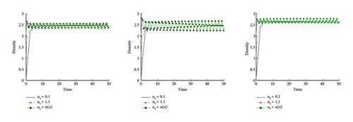
Example 1. We consider (1) on Ω ≡ x = (0, 1) with D = 1.0, harvesting H = 0.0, carrying capacity and different intrinsic growth rates r = 1.2, 1.2 + cos(πx), 1.2 + cos(πx)sin(πt). The numerical simulation in Figure 1 shows that in the absence of harvesting, we get a unique positive periodic solution whatever the initial density point is. Moreover, the result shows similar behavior in two dimensions (Figure 2). It is time to establish the unique solution for any initial density maps and for various growth rates. The existence and uniqueness of the solution of (1) are valid as designed in Figures 1 and 2. These figures justified the result of Theorem 1.

Details are in the caption following the image — **Figure 1**
Open in figure viewer PowerPoint

Solution of (1) for H = 0.0, , D = 1, u₀ = {0.1, 1.1, 2.0 + sin(πx)}, (left) r = 1.2, (middle) r(x) = 1.2 + cos(πx) and (right) r(x, t) = 1.2 + cos(πx)sin(πt).

Example 2. Consider (1) on Ω = (0, 1) with D = 1.0 and H = 0.0, time variable carrying capacity and initial population u₀(x) = 2.0 + sin(πx). For time-periodic carrying capacity and for various growth functions, the numerical simulation shows a positive unique solution. The equilibrium depends on the change of intrinsic growth rates r = 1.2, 1.2 + cos(πx), 1.2 + cos(πx)sin(πt) which is shown in left figure of Figure 3. Also in right figure of Figure 3, explains the uniqueness of the positive solution despite of different initial mass.

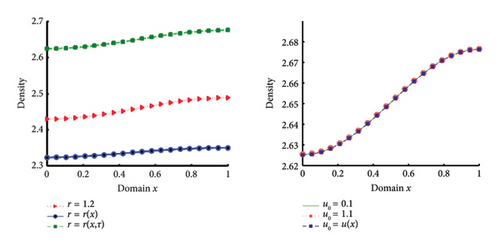
In both cases (Case 1 and Case 2), Theorem 1 is verified for random time-periodic carrying capacity functions . In the next example, we outline the impact of the dispersal coefficients D on the steady state level.

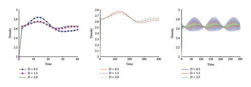
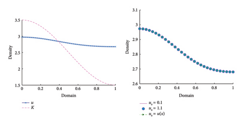
Example 3. Consider model (1) with time variable carrying capacity and intrinsic growth rate r(x, t) = 1.2 + cos(πx)sin(πt). Also consider H = 0, initial population density u₀ = 1.1 for Ω = (0, 1). Numerically, it shows that the value of u(x, t) converges to the time periodic positive solution when t⟶∞. The more we increase the diffusion strategy, that is, increasing of D, the more we converge to the limit state for the same initial density and t > 0. See the illustration of Figure 4. There is a similar illustration in Figure 5 for a two-dimensional scenario. Finally, if we consider , carrying capacity only dependent on the environment, then we get a unique positive solution as shown in Figure 6.

Now, we consider the case with harvesting in (1). Here, first explore the behavior in the absence of diffusion.

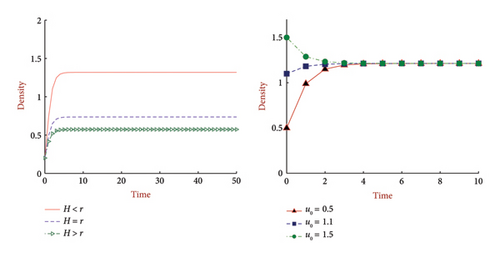
Example 4. Let us consider model (1) in absence of diffusion, which is equivalent to (3) over the domain Ω = (0, 1). Since the diffusion is absent, so for D = 0 and the constant coefficients are constant. We verify the results of subsection 3.1. First we choose different values of harvesting rate H = {0.5, 1.2, 1.5} with growth rate r = 1.2 and carrying capacity . This shows that the results found in subsection 3.1 is justified. We also check for different initial values with a fixed harvesting rate, where the results are justified. See Figure 7.

Example 5. Consider model (6) over Ω = (0, 1) and for D = 0.0. The coefficients are all time dependent, that is functions of time t. For growth rates r(t) = 1.3 + cos t, carrying capacity and different values of harvesting rates (H = {1.1 + cos t, 1.3 + cos t, 1.5 + cos t} in Figure 8 (left)) and initial densities (u₀ = {0.3, 1.1, 1.7} with H = 1.2 + cos t in Figure 8 (right)), we observe the solution of (6). If we take smooth functions in the coefficients we get a unique positive T-periodic solution of equation (6).

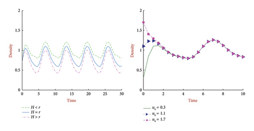
In the above two cases (Case 4 and Case 5; Figures 7 and 8), we verify the results in Section 3 for constant coefficients and time dependent coefficients, respectively.

In both cases, we have a delicate value H = r, which leads two different phases, either the population will persist or extinct under harvesting absorption. We also get a unique positive solution for H < r, whatever the starting point is.

Example 6. Consider equation (1) with all coefficients are only spatially distributed such that, which satisfies (∂u/∂η)|_∂Ω = 0, which is discussed with the model (10).

Here, the supreme population consistency level is

. Moreover,

()

After a long time period, t⟶+∞, for u₀(x) > 0 the solution u(t, x; u₀) tends to the optimal solution u^∗(x). Therefore, the similar maximum sustainable outcome for unit time is

()

The last inequality follows from the Green’s theorem [37]. Now, we explore the behavior of equation (10) in Figure 9 for D = 1.0, , u₀(x) = 0.5 + sin²(πx), r(x) = 1.5 + cos(πx)sin(x), and H(x) = 0.75 + cos²(πx) on Ω = (0, 1) for t = (0, 100) and it verifies the result of Theorem 2.

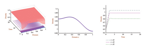
Example 7. Consider model (1) over the region Ω = (0, 1) with D = 1.0, carrying capacity and intrinsic growth rate r(x, t) = 1.2 + cos(πx)sin(πt).

We choose different harvesting rates H(x, t) = 0.75 + cos²(πx)sin(πt) < r(x, t), 1.2 + cos(πx)sin(πt) = r(x, t), 1.5 + cos(πx)sin(πt) > r(x, t).

The numerical simulation shows we get a unique positive periodic solution and explore the equilibrium on the change of intrinsic growth rates and harvesting rates.

In this example (Figure 10), Theorem 1 is verified for random time-periodic carrying capacity functions .

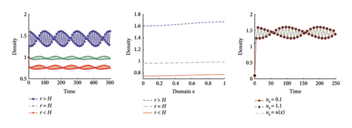
Now, we outline the significance of the dispersal coefficients D on the steady state level. With the increase of D, the convergence of the solution is faster than the limit state for the same initial density and t > 0.

Consider model (1) for various diffusion such as D = {0.5, 1.5, 2.5} with time varying carrying capacity , intrinsic growth rate r(x, t) = 1.2 + cos(πx)sin(πt), harvesting rate H(x, t) = 0.75 + cos²(πx)sin(πt) with initial population u₀(x) = 1.0 + sin(πx). Figure 11 illustrates the speed of convergence clearly.

In all our numerical simulations, we used MATLAB, a high-level programming and numeric computing platform, to generate the figures presented in this paper. This software facilitated the precise rendering of data visualizations, ensuring accuracy, and clarity in demonstrating our results.

9. Conclusion

In this study, we have studied a reaction-diffusion model for a single species population model with Gompertz growth law, where all parameters such as capacity map, intrinsic growth rate, and harvesting rate are spatially time distributed. In particular, it was demonstrated that a solution of the given model (1) exists and is unique. It has been established that the solution is positive for any non-negative and nonzero initial function for an open-bounded nonempty domain. All solutions of (1) converge to the positive steady state using upper-lower solution techniques for the model with time-dependent carrying capacity. The model’s and solution’s validity are also verified for time-independent carrying capacity. To optimize the population density, we have used the technique of variational calculus. However, if parameters are positive and periodic in t-functions rather than t-independent parameters, then certain restrictions on r(x, t), H(x, t) and

are imposed in Theorem 3 and we get the optimal sustainable yield. The condition that the intrinsic growth rate exceeds the supremum of the relative change of the carrying capacity in time

means that the growth rate can compensate for the change in the carrying capacity. This restriction frequently occurs in the problems of optimal harvesting. We find the optimum harvesting strategy for Gompertz law in this paper. We also generalized the results using multiple growth functions with harvesting. We presented numerical examples to justify the analytic results for various parametric values in a nonempty open domain with different initial conditions. The problem can be extended for

1.
Noncommunicable disease modeling, like tumor and cancer modeling since Gompertz law is specified as a highly increasing function in a certain density level
2.
Toxic problem in ecology and infections for multiple plants
3.
Delay type differential problems; and
4.
Introducing homogeneous and nonhomogeneous Dirichlet boundary conditions.

Additionally, future research could further explore the integration of economic controls, such as those described by Chatterjee and Pal, into ecological models to enhance sustainability and resource optimization [45].

Ethics Statement

No consent is required to publish this manuscript.

Conflicts of Interest

The authors declare no conflicts of interest.

Author Contributions

Conceptualization, M.K. and S.I.A.; methodology, K.N.K., M.H.A.B., and K.M.A.K.; software, M.K. and S.I.A.; validation, M.H.A.B. and M.R.I.; formal analysis, M.K, S.I.A. and M.R.I.; investigation, K.N.K. and K.M.A.K.; resources, K.N.K. and M.R.I.; data curation, S.I.A.; original draft preparation, M.K. and S.I.A.; review and editing, M.H.A.B. and M.R.I. and K.M.A.K.; supervision, M.K. All authors have read and agreed to the published version of the manuscript.

Funding

The research by Md. Kamrujjaman was both financially and non financially supported by the University Grant Commission (UGC), and the University of Dhaka, Bangladesh.

Open Research

Data Availability Statement

Data sharing is not applicable to this article as no new data were created or analyzed in this study.

References

1 Turing A. M., The Chemical Basis of Morphogenesis, Philosophical Transactions of the Royal Society of London-B. (1952) 237, 37–72.
10.1098/rstb.1952.0012
CAS Web of Science® Google Scholar
2 Holmes E. E., Lewis M. A., Banks J. E., and Veit R. R., Partial Differential Equations in Ecology: Spatial Interactions and Population Dynamics, Ecology. (1994) 75, no. 1, 17–29, https://doi.org/10.2307/1939378.
10.2307/1939378
Web of Science® Google Scholar
3 Murray J. D., Stanley E. A., and Brown D. L., On the Spatial Spread of Rabies Among Foxes, Proceedings of the Royal Society of London-Series B: Biological Sciences. (1986) 229, no. 1255, 111–150, https://doi.org/10.1098/rspb.1986.0078.
10.1098/rspb.1986.0078
CAS PubMed Web of Science® Google Scholar
4 Chaplain M. A. J., Reaction-Diffusion Pre-Patterning and Its Potential Role in Tumor Invasion, Journal of Biological Systems. (1995) 3, no. 4, 929–936.
10.1142/S0218339095000824
Google Scholar
5 Sheergojri A. R., Iqbal P., Agarwal P., and Özdemir N., Uncertainty-Based Gompertz Growth Model for Tumor Population and Its Numerical Analysis, An International Journal of Optimization and Control: Theories & Applications. (2022) 12, no. 2, 137–150, https://doi.org/10.11121/ijocta.2022.1208.
10.11121/ijocta.2022.1208
Google Scholar
6 Braverman E. and Kamrujjaman M., Competitive–Cooperative Models With Various Diffusion Strategies, Computers & Mathematics With Applications. (2016) 72, no. 3, 653–662, https://doi.org/10.1016/j.camwa.2016.05.017.
10.1016/j.camwa.2016.05.017
Web of Science® Google Scholar
7 Braverman E. and Kamrujjaman M., Lotka Systems With Directed Dispersal Dynamics: Competition and Influence of Diffusion Strategies, Mathematical Biosciences. (2016) 279, 1–12, https://doi.org/10.1016/j.mbs.2016.06.007.
10.1016/j.mbs.2016.06.007
CAS PubMed Web of Science® Google Scholar
8 Bai L. and Wang K., A Diffusive Single-Species Model With Periodic Coefficients and Its Optimal Harvesting Policy, Applied Mathematics and Computation. (2007) 187, no. 2, 873–882, https://doi.org/10.1016/j.amc.2006.09.007.
10.1016/j.amc.2006.09.007
Web of Science® Google Scholar
9 Cosner C., A. Friedman, Reaction-Diffusion Equations and Ecological Modeling, Tutorials in Mathematical Biosciences IV (Evolution and Ecology), 1922, Springer.
Google Scholar
10 Zhao X. Q., Dynamical System in Population Biology, 2003, Springer, Verlag, New York, NY.
10.1007/978-0-387-21761-1
Google Scholar
11 Masti I., Sayevand K., and Jafari H., On Analyzing Two Dimensional Fractional Order Brain Tumor Model Based on Orthonormal Bernoulli Polynomials and Newton’s Method, An International Journal of Optimization and Control: Theories & Applications. (2024) 14, no. 1, 12–19.
Google Scholar
12 Kuang Y., Delay Differential Equations With Applications in Population Dynamics, Mathematics in Science and Engineering. (1993) 191.
Google Scholar
13 Cantrell R. S. and Cosner C., Spatial Ecology Via Reaction-Diffusion Equations, Wiley Series in Mathematical and Computational Biology. (2003) John Wiley and Sons, Chichester.
Google Scholar
14 Kamrujjaman M., Directed Vs Regular Diffusion Strategy: Evolutionary Stability Analysis of a Competition Model and an Ideal Free Pair, Differential Equations & Applications. (2019) 11, no. 2, 267–290, https://doi.org/10.7153/dea-2019-11-11.
10.7153/dea-2019-11-11
Google Scholar
15 Kamrujjaman M., Interplay of Resource Distributions and Diffusion Strategies for Spatially Heterogeneous Populations, Journal of Mathematical Modeling. (2019) 7, no. 2, 175–198.
Google Scholar
16 Korobenko L., Kamrujjaman M., and Braverman E., Persistence and Extinction in Spatial Models With a Carrying Capacity Driven Diffusion and Harvesting, Journal of Mathematical Analysis and Applications. (2013) 399, no. 1, 352–368, https://doi.org/10.1016/j.jmaa.2012.09.057.
10.1016/j.jmaa.2012.09.057
Web of Science® Google Scholar
17 Braverman E. and Braverman L., Optimal Harvesting of Diffusive Models in a Non-Homogeneous Environment, Nonlinear Analysis: Theory, Methods & Applications. (2009) 71, no. 12, e2173–e2181, https://doi.org/10.1016/j.na.2009.04.025.
10.1016/j.na.2009.04.025
Google Scholar
18 Adan M. M. I. Y., Kamrujjaman M., Molla M. M., Mohebujjaman M., and Buenrostro C., Interplay of Harvesting and the Growth Rate for Spatially Diversified Populations and the Testing of a Decoupled Scheme, Mathematical Biosciences and Engineering. (2023) 20, no. 4, 6374–6399, https://doi.org/10.3934/mbe.2023276.
10.3934/mbe.2023276
PubMed Web of Science® Google Scholar
19 Henson S. M. and Cushing J. M., The Effect of Periodic Habitat Fluctuations on a Nonlinear Insect Population Model, Journal of Mathematical Biology. (1997) 36, no. 2, 201–226, https://doi.org/10.1007/s002850050098.
10.1007/s002850050098
Web of Science® Google Scholar
20 Xu C., Boyce M. S., and Daley D. J., Harvesting in Seasonal Environments, Journal of Mathematical Biology. (2005) 50, no. 6, 663–682, https://doi.org/10.1007/s00285-004-0303-5.
10.1007/s00285-004-0303-5
PubMed Web of Science® Google Scholar
21 Gompertz B., On the Nature of the Function Expressive of the Law of Human Mortality, and on a New Mode of Determining the Value of Life Contingencies, Philosophical Transactions of the Royal Society of London. (1825) 115, 513–583.
10.1098/rstl.1825.0026
Google Scholar
22 Winsor C. P., The Gompertz Curve as a Growth Curve, Proceedings of the National Academy of Sciences. (1932) 18, 1–8, https://doi.org/10.1073/pnas.18.1.1.
10.1073/pnas.18.1.1
CAS PubMed Web of Science® Google Scholar
23 Wright S., Pearl R., and Sweeney J. S., The Biology of Population Growth, Journal of the American Statistical Association. (1926) 21, no. 156, 493–497, https://doi.org/10.2307/2276990.
10.2307/2276990
Google Scholar
24 Starck J. M. and Ricklefs R. E., Avian Growth and Development: The Evolution Within the Altricial-Precocial Spectrum, 1998, Oxford University Press, New York.
Google Scholar
25 Ricker W. E., W. S. Hoar, D. J. Randall, and J. R. Brett, Growth Rates and Models, Fish Physiology, 1979, Academic Press, London, 677–743.
10.1016/S1546-5098(08)60034-5
Web of Science® Google Scholar
26 Paine C. E. T., Marthews T. R., Vogt D. R. et al., How to Fit Nonlinear Plant Growth Models and Calculate Growth Rates: An Update for Ecologists, Methods in Ecology and Evolution. (2012) 3, no. 2, 245–256, https://doi.org/10.1111/j.2041-210x.2011.00155.x.
10.1111/j.2041-210x.2011.00155.x
Web of Science® Google Scholar
27 Zwietering M. H., Jongenburger I., Rombouts F. M., and Van’T Riet K., Modeling of the Bacterial Growth Curve, Applied and Environmental Microbiology. (1990) 56, no. 6, 1875–1881, https://doi.org/10.1128/aem.56.6.1875-1881.1990.
10.1128/aem.56.6.1875-1881.1990
CAS PubMed Web of Science® Google Scholar
28 Skinner G. E., Larkin J. W., and Rhodehamel E. J., Mathematical Modeling of Microbial Growth: A Review, Journal of Food Safety. (1994) 14, no. 3, 175–217, https://doi.org/10.1111/j.1745-4565.1994.tb00594.x.
10.1111/j.1745-4565.1994.tb00594.x
Web of Science® Google Scholar
29 Laird A. K., Dynamics of Tumor Growth, British Journal of Cancer. (1964) 18, no. 3, 490–502, https://doi.org/10.1038/bjc.1964.55.
10.1038/bjc.1964.55
Web of Science® Google Scholar
30 Kawasaki K., Mochizuki A., Matsushita M., Umeda T., and Shigesada N., Modeling Spatio-Temporal Patterns Generated by Bacillus Subtilis, Journal of Theoretical Biology. (1997) 188, no. 2, 177–185, https://doi.org/10.1006/jtbi.1997.0462.
10.1006/jtbi.1997.0462
CAS PubMed Web of Science® Google Scholar
31 Murray J. D., Mathematical Biology. II: Spatial Models and Biomedical Applications, 2003, Springer, New York.
10.1007/b98869
Google Scholar
32 Wu Y. and Zhao X. Q., The Existence and Stability of Travelling Waves With Transition Layers for Some Singular Cross-Diffusion Systems, Physica D: Nonlinear Phenomena. (2005) 200, no. 3-4, 325–358, https://doi.org/10.1016/j.physd.2004.11.010.
10.1016/j.physd.2004.11.010
Web of Science® Google Scholar
33 Zahan I. and Kamrujjaman M., Evolution of Dispersal and the Analysis of a Resource Flourished Population Model With Harvesting, Heliyon. (2024) 10, https://doi.org/10.1016/j.heliyon.2024.e30737.
10.1016/j.heliyon.2024.e30737
Web of Science® Google Scholar
34 Mohebujjaman M., Buenrostro C., Kamrujjaman M., and Khan T., Decoupled Algorithms for Non-Linearly Coupled Reaction-Diffusion Competition Model With Harvesting and Stocking, Journal of Computational and Applied Mathematics. (2024) 436, https://doi.org/10.1016/j.cam.2023.115421.
10.1016/j.cam.2023.115421
Web of Science® Google Scholar
35 Clark C. W., Mathematical Bio-Economics: The Optimal Management of Renewable Resources, 1990, Wiley, New York, NY.
Google Scholar
36 Fan M. and Wang K., Optimal Harvesting Policy for Single Population With Periodic Coefficients, Mathematical Biosciences. (1998) 152, no. 2, 165–178, https://doi.org/10.1016/s0025-5564(98)10024-x.
10.1016/s0025-5564(98)10024-x
CAS PubMed Web of Science® Google Scholar
37 Li H., A Class of Single-Species Models With Periodic Coefficients and Their Optimal Harvesting Policy, Journal of Biomathematics. (1999) 14, no. 4, 479–483.
Google Scholar
38 Zahan I., Kamrujjaman M., and Tanveer S., Mathematical Study of a Resource Based Diffusion Model With Gilpin-Ayala Growth and Harvesting, Bulletin of Mathematical Biology. (2022) 84, no. 10, https://doi.org/10.1007/s11538-022-01074-8.
10.1007/s11538-022-01074-8
PubMed Web of Science® Google Scholar
39 Kamrujjaman M., Keya K. N., Bulut U., Islam M. R., and Mohebujjaman M., Spatio-Temporal Solutions of a Diffusive Directed Dynamics Model With Harvesting, Journal of Applied Mathematics and Computing. (2023) 69, no. 1, 603–630, https://doi.org/10.1007/s12190-022-01742-x.
10.1007/s12190-022-01742-x
PubMed Web of Science® Google Scholar
40 Pinch E. R., Optimal Control and the Calculus of Variations, 1993, Oxford University Press, New York.
10.1093/oso/9780198532170.001.0001
Google Scholar
41 Lu H. and Wang K., An Autonomous Single-Species Model and Their Optimal Harvesting Policy, Journal of Systems Mathematical Sciences. (2004) 24, no. 4, 200–205.
Google Scholar
42 Zhou L. and Fu Y., Existence and Stability of Periodic Quasisolutions in Nonlinear Parabolic Systems With Discrete Delays, Journal of Mathematical Analysis and Applications. (2000) 250, no. 1, 139–161, https://doi.org/10.1006/jmaa.2000.6986.
10.1006/jmaa.2000.6986
Web of Science® Google Scholar
43 Su J. and Pan J., Functional Analysis and Variational Calculus, 1993, Press of Technology and Science University, Hefei.
Google Scholar
44 Gelfand I. M. and Fomin S. V., Calculus of Variations, 1963, Dover Publications, New York.
Google Scholar
45 Chatterjee A. and Pal S., A Predator-Prey Model for the Optimal Control of Fish Harvesting Through the Imposition of a Tax, An International Journal of Optimization and Control: Theories & Applications. (2023) 13, no. 1, 68–80, https://doi.org/10.11121/ijocta.2023.1218.
10.11121/ijocta.2023.1218
Google Scholar

All articles

Mathematical Analysis of a Resource-Based Dispersal Model With Gompertz Growth and Optimal Harvesting

Abstract

1. Introduction

2. Model and Methods

3. Dynamics of Time Periodicity

3.1. Dynamics for Constant Coefficients

3.2. Dynamics for Time-Periodic Coefficients

3.2.1. Determination of Maximum Harvesting Yield

4. Classical Diffusion With Harvesting

5. Uniqueness and Existence of a Periodic Solution

6. Sustainable Yield With Optimal Policy

7. Classical Diffusion With Generalized Growth Function

8. Numerical Simulation

9. Conclusion

Ethics Statement

Conflicts of Interest

Author Contributions

Funding

Open Research

Data Availability Statement

References

Figures

References

Information

About Wiley Online Library

Help & Support

Opportunities

Connect with Wiley

Mathematical Analysis of a Resource-Based Dispersal Model With Gompertz Growth and Optimal Harvesting

Abstract

1. Introduction

2. Model and Methods

3. Dynamics of Time Periodicity

3.1. Dynamics for Constant Coefficients

3.2. Dynamics for Time-Periodic Coefficients

3.2.1. Determination of Maximum Harvesting Yield

4. Classical Diffusion With Harvesting

5. Uniqueness and Existence of a Periodic Solution

6. Sustainable Yield With Optimal Policy

7. Classical Diffusion With Generalized Growth Function

8. Numerical Simulation

9. Conclusion

Ethics Statement

Conflicts of Interest

Author Contributions

Funding

Open Research

Data Availability Statement

References

Figures

References

Related

Information