International Journal of Antennas and Propagation

Volume 2025, Issue 1 1126365

Research Article

Open Access

Research on the Macrocell Wireless Channel Model Based on Physic-Inspired Support Vector Regression Algorithm Wireless Channel Model in Macrocell Environment

Qi Yao,

Qi Yao

orcid.org/0000-0002-0733-3786

School of Physics , Xidian University , Xi’an , 710071 , Shaanxi, China , xidian.edu.cn

Search for more papers by this author

Zhongyu Liu,

Corresponding Author

Zhongyu Liu

[email protected]

orcid.org/0009-0003-1611-3130

School of Physics , Xidian University , Xi’an , 710071 , Shaanxi, China , xidian.edu.cn

Search for more papers by this author

Lixin Guo,

Lixin Guo

School of Physics , Xidian University , Xi’an , 710071 , Shaanxi, China , xidian.edu.cn

Search for more papers by this author

Jiang Guo,

Jiang Guo

School of Physics , Xidian University , Xi’an , 710071 , Shaanxi, China , xidian.edu.cn

Search for more papers by this author

Zuoyong Nan,

Zuoyong Nan

China Information Technology Designing & Consulting Institute Co. Ltd. , Beijing , 100080 , China

Search for more papers by this author

Wei Liu,

Wei Liu

School of Physics , Xidian University , Xi’an , 710071 , Shaanxi, China , xidian.edu.cn

Search for more papers by this author

Jiangting Li,

Jiangting Li

School of Physics , Xidian University , Xi’an , 710071 , Shaanxi, China , xidian.edu.cn

Search for more papers by this author

Qi Yao,

Qi Yao

orcid.org/0000-0002-0733-3786

School of Physics , Xidian University , Xi’an , 710071 , Shaanxi, China , xidian.edu.cn

Search for more papers by this author

Zhongyu Liu,

Corresponding Author

Zhongyu Liu

[email protected]

orcid.org/0009-0003-1611-3130

School of Physics , Xidian University , Xi’an , 710071 , Shaanxi, China , xidian.edu.cn

Search for more papers by this author

Lixin Guo,

Lixin Guo

School of Physics , Xidian University , Xi’an , 710071 , Shaanxi, China , xidian.edu.cn

Search for more papers by this author

Jiang Guo,

Jiang Guo

School of Physics , Xidian University , Xi’an , 710071 , Shaanxi, China , xidian.edu.cn

Search for more papers by this author

Zuoyong Nan,

Zuoyong Nan

China Information Technology Designing & Consulting Institute Co. Ltd. , Beijing , 100080 , China

Search for more papers by this author

Wei Liu,

Wei Liu

School of Physics , Xidian University , Xi’an , 710071 , Shaanxi, China , xidian.edu.cn

Search for more papers by this author

Jiangting Li,

Jiangting Li

School of Physics , Xidian University , Xi’an , 710071 , Shaanxi, China , xidian.edu.cn

Search for more papers by this author

First published: 01 July 2025

https://doi.org/10.1155/ijap/1126365

Academic Editor: Rajashik Paul

Share a link

Email
Wechat
Bluesky

Abstract

To support wireless network planning and optimization in macrocellular environments, this paper presents an efficient machine learning method capable of achieving rapid predictive simulations at the kilometer level. The method embeds the building transmission model (BTM) into a machine learning framework based on support vector regression. The core of this new regression model lies in mapping the antenna and environmental feature information through the BTM into a high-dimensional space and then seeking the optimal hyperplane in this space that maximizes the margin with respect to the training data. In addition, a model was constructed and validated based on measured wireless channel data at frequencies of 900 and 3500 MHz. The results show that the root mean square error between the proposed model and the measured results is less than 7 dB, and the single-point simulation time of the proposed model for kilometer-scale large-scale coverage prediction is in the millisecond range.

1. Introduction

The efficient planning of macrocell [1] networks is considered to be a key cornerstone toward a green network [2–4], which requires accurate and reliable radio wave propagation modeling. For this task, researchers have developed many wireless channel prediction models for macrocells over the years. These models are generally divided into two categories: statistical models and deterministic models.

The statistical model [5–7] is developed by conducting extensive experimental measurements in different regions and utilizing statistical analysis to fit the propagation characteristics of other regions. Therefore, statistical models are simple and have fast computation speed, but their accuracy is not high [8, 9]. Different models should be studied for different scenarios, and the most similar model developed in a similar region should be used to achieve high accuracy [10, 11]. Deterministic models [12–14] rely on environmental features such as operating frequency, building type, obstructions, and precise geometric information of buildings, as well as material types of all measured areas [15, 16]. Such models use a large number of simulations to estimate the effects of scattering, refraction, and reflection on transmitted signals. Therefore, deterministic models are usually very complex, with slow computation speed, and the accuracy of computation is affected by the accuracy of environmental information [17–19]. In view of the limitations of both approaches, an increasing number of researchers have started to employ machine learning-based techniques [20, 21] for constructing wireless channel prediction models in macrocellular environments. The aim is to achieve computational efficiency, high prediction accuracy, and strong generality in electromagnetic wave propagation models.

1.1. Related Works

In reference [22], the optimal structure for artificial neural network-based wireless channel prediction model for urban environments was proposed, and their research results showed that as long as the size of the neural network is chosen correctly, the path loss model based on artificial neural networks can be effectively executed. In reference [23], the combination of image-based environmental representation methods and artificial neural networks can enhance path loss prediction in terms of accuracy and efficiency. In reference [24], a deep learning-based method was proposed to achieve accurate prediction of millimeter wave path loss. In reference [25], a general framework was proposed for training neural networks to predict path loss but without considering environmental information.

2. Challenges and Proposed Methods

On the whole, from the perspective of service providers, most of these previous efforts have limitations and concerns in terms of their actual implementation and acceptable accuracy.

1.
Currently, most studies use ray tracing as a reference, which may lead to inaccurate and impractical problems. Relying solely on ray tracing for comparisons cannot accurately measure acceptable coverage prediction accuracy. To the best of our knowledge, there has been no extensive drive test data work conducted in a large geographic area with multiple base stations that can serve as a reference for comparison to determine the actual results that have a significant impact on service provider plans.
2.
Most previous research has been entirely based on satellite maps, lacking support for universal data models such as triangulation networks. This limitation hinders the practical implementation of research findings.
3.
In the past, research in macrocellular environments has largely focused on extracting features based on scene and antenna information for direct use in machine learning training and prediction. However, these approaches often lack support from physical mechanisms, leading to poor model generalizability.

In order to address these limitations, this paper aims to explore and validate a macrocell wireless channel prediction model based on physically inspired support vector regression (SVR) algorithms. It is expected that the proposed model will significantly improve prediction accuracy, computational efficiency, and generality. The physical heuristic method combines a deep understanding of the physical characteristics of the channel to guide the construction and optimization of machine learning models. Insights gained from physical processes are used to effectively capture and utilize the nonlinear dynamic characteristics of the channel while also significantly reducing overfitting issues in data-driven methods, thereby improving the generalization ability and robustness of the prediction model.

In order to consider the impact of environmental geometric and electrical parameter information on radio wave propagation, this paper selects the building transmission model (BTM) [26] as an interpreter for the wireless radio wave propagation mechanism in macrocellular environments. BTM has been proven to be reliable [27–29]. In order to achieve the following goals: (1) better performance in handling noisy and anomalous data; (2) ability to handle complex nonlinear relationships; (3) fast training and prediction computation; and (4) easy integration with physical mechanisms. In the commonly used machine learning methods, this paper selects SVR [30] as the machine learning framework. SVR has its strong nonlinear modeling ability, robustness, ability to handle outliers, and effective generalization ability, which have made it widely used and recognized in practical applications [31–33].

The primary contributions and innovations of this paper are summarized as follows:

1.
Embedding BTM into a machine learning framework based on SVR, the feature information of the antenna and environment is mapped into a high-dimensional space through BTM. In this space, an optimal hyperplane is sought to maximize the margin between the hyperplane and the training data, resulting in a new regression model referred to as BTM–SVR in this paper.
2.
Based on a comparative analysis with a large amount of measured data, this study systematically investigates the impact of attenuation coefficients and the number of support vectors on the accuracy, training time, and prediction time of BTM–SVR. The optimal attenuation coefficient and number of support vectors that balance accuracy and efficiency in macrocell environments are quantified.
3.
The combination of the BTM feature extraction algorithm for general scenarios and BTM–SVR has enabled the simulation of kilometer-level coverage prediction in macrocell environments. Based on the optimal attenuation coefficient and number of support vectors obtained, an efficient coverage prediction simulation model has been developed.

The remaining sections of this paper are organized as follows. Section 2 provides a detailed introduction to the theoretical approach and construction steps of BTM–SVR. In Section 3, the measurement activities are described and the measurement data is analyzed. The optimization and numerical analysis of BTM–SVR are presented in Section 4. Finally, conclusions are drawn in Section 5.

2.1. Propagation Model

The objective here is to integrate the wireless radio wave propagation mechanism into the SVR architecture within a macrocellular environment, with the aim of achieving efficient and rapid prediction of received power. This paper adopts BTM as a method for predicting wireless radio wave propagation in macrocellular environments. BTM is a semideterministic and semiempirical model that considers multiple influencing factors in the process of radio wave propagation while also being capable of rapidly solving these factors. Therefore, BTM is used as the sample mapping function for the kernel function in the SVR method, which satisfies the radio wave propagation mechanism in macrocell environments and achieves a fast computing speed.

2.1.1. The Theoretical Framework of BTM–SVR

In a macrocell environment, BTM is a radio wave propagation model that can better explain the main transmission mechanism. The model relies on prior knowledge of the exterior coordinates of the building, its dielectric constant, and a decay factor related to the overall field behavior within the building. The attenuation coefficient of a single building can be estimated by measuring the introduced attenuation of the propagating signal as it passes through the building. For real urban microcell scenarios, the method greatly enhances the efficiency of path loss prediction by taking into account the penetration and transmission of buildings.

When radio waves pass through buildings, it is necessary to understand the field distribution within the structure in order to evaluate the path loss. However, the distribution of the field depends on various parameters such as building materials, internal layout, and shape, which are not always readily available. Therefore, in order to capture the overall behavior of the internal field and the transmitted field, a specific attenuation coefficient α_b was determined. A schematic diagram of the BTM for multiple buildings is shown in Figure 1. In order to predict the excessive loss caused by the penetration phenomenon (L_T) in multiple buildings, the formula is as follows [26]:

()

Details are in the caption following the image — **Figure 1**
Open in figure viewer PowerPoint

Schematic diagram of BTM under multiple buildings.

In the formula, j represents the building identifier, n represents the number of buildings passed from the transmitter to the receiver, α_b represents the attenuation coefficient of the building,

represents the path length for radio wave propagation within the jth building, T(r) represents the transmission coefficient,

and

represent the first and last transmission points where the radio wave reaches the jth building surface. The transmission coefficient T(r) is calculated according to following equation:

()

Among them, r₀ is an arbitrary transmission point on the surface of the building, R(r₀) is the reflection coefficient, ε_r is the relative dielectric constant of the building medium, and θ_i,0 is the incident angle. The reflection coefficient R(r₀) links the amplitude of the incident field with that of the complex reflected field. According to the BTM, the received power at Rx is

()

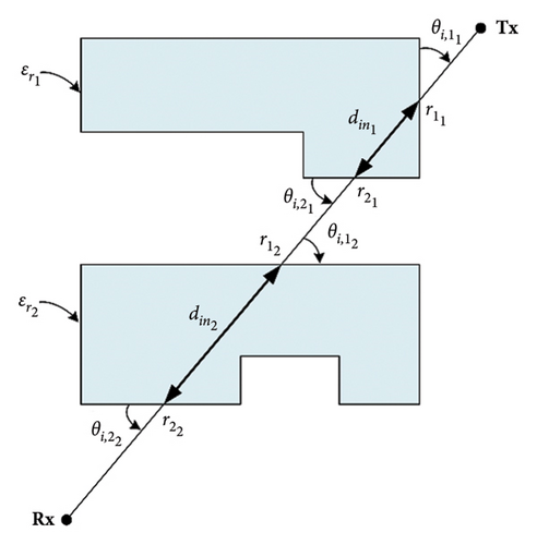
In the equation, P_t denotes the transmission power, G_t and G_r represent the antenna gains of Tx and Rx, c stands for the propagation speed of electromagnetic waves, f represents the frequency of the electromagnetic wave, and d signifies the distance between Tx and Rx.

In order to integrate the radio wave propagation mechanism into the SVR architecture, the feature information and received power between each Tx and Rx are constructed as a sample, with the feature value x defined as follows:

()

Clearly, the feature value x of each sample can be mapped to a corresponding P_r denoted as follows:

()

Then, the prediction function of sample x_j based on the SVR algorithm is as follows:

()

where x_i represents the feature value of the corresponding support vector, m denotes the number of support vectors,

is the Lagrange multiplier, and b signifies the offset. Determining the most suitable “distance” between samples is of great importance in the field of machine learning. In equation (8), z represents the method for calculating the distance between two samples. In subsequent research, z = 2. It is worth mentioning that unlike traditional kernel functions, the data corresponding to equation (8) represent real physical quantities rather than normalized values.

During the training process, the main goal is to solve for α^∗ and b. The problem is transformed into a minimization problem in the following form:

()

where y_j represents the actual received power of sample x_j, and k denotes the number of training samples.

The detailed process of solving for α^∗ and b is as follows:

()

Let

, and

, then

()

Let

, and rewrite equations (11) and (12) as follows:

()

It is worth mentioning that the reflection coefficient is used in the calculation of the transmission information obtained according to BTM, which links the influence of the material of the building on the radio wave propagation, so that the proposed model can consider the influence of different materials, which is not available in many traditional algorithms. In addition, to assess the performance of BTM–SVR, two error metrics were employed: the mean absolute error (MAE) and the root mean square error (RMSE), defined as follows:

()

where y(i) represents the actual result of the ith sample, and y_p(i) represents the predicted result of the ith sample.

2.1.2. Constructing BTM–SVR

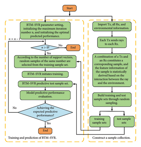
The process of constructing the BTM–SVR is illustrated in Figure 2, with detailed steps outlined as follows.

Step 1: import Tx, Rx, and environmental data.
Step 2: rays are emitted from each Tx to each Rx, and feature information is extracted from the interaction between the rays and the environment to construct a sample set. In the subsequent research of this paper, 30% of the sample set will be randomly selected as the training sample set, with the remainder forming the test sample set.
Step 3: initialize the BTM–SVR parameter settings, set the maximum number of iterations n, and initialize the best predictive performance.
Step 4: if n > 0, proceed to Step 5; otherwise, terminate the execution.
Step 5: train the BTM–SVR by randomly selecting a corresponding number of samples from the training sample set based on the number of support vectors.
Step 6: predict the outcomes of the test sample set using the trained model. Compare these predictions with the actual measured results. If the expected predictive performance is achieved, terminate the process; otherwise, set n = n-1 and proceed to Step 4.

According to equation (5), the input sample features that need to be extracted from parameters of Tx, Rx, and environment are as follows: (1) the total number of buildings between Tx and Rx; (2) the sum of radio wave propagation paths within buildings between Tx and Rx; (3) the incident angles on surfaces of individual buildings; (4) the average permittivity of buildings between Tx and Rx; (5) the straight-line distance between Tx and Rx; (6) the radio wave frequency; (7) the tilt angle of Rx relative to Tx; (8) the power of Tx; and (9) the gains of both Tx and Rx. The output feature is received power.

From the construction steps, it can be observed that BTM–SVR possesses the following advantages: (1) BTM–SVR requires a small number of features that are easy to obtain and involves fewer matrix parameters, resulting in fast computation speed; (2) in comparison to typical machine learning methods, BTM–SVR does not necessitate data normalization; and (3) BTM–SVR is capable of predicting both path loss and received power.

2.1.3. Experimental Measurement Activity

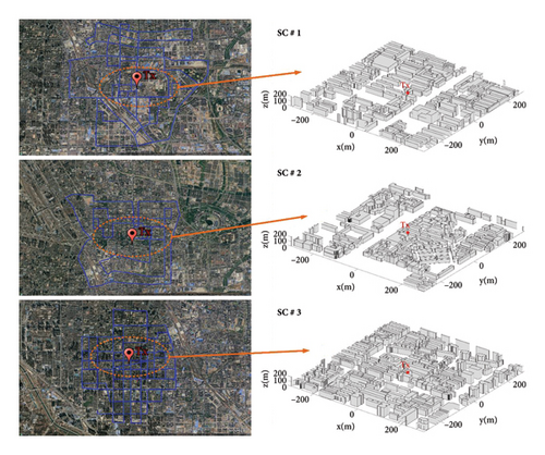
The development of BTM–SVR proposed in this research is based on experimental data collected during measurement activities conducted in Zhengzhou City, China. The satellite map of the measurement area is shown in Figure 3, with a longitude range from 113°35′E to 113°45′E and a latitude range from 34°41′N to 34°52′N. The specific measurement groups are shown in Table 1. The electromagnetic wave frequencies measured were 900 MHz and 3500 MHz, and the method for measuring received signals was referenced from literature [34]. Both Tx and Rx utilize conical antennas of model PZ-100800/P, manufactured by Ainfoinc. These antennas cover a frequency range of 1–8 GHz and exhibit an omnidirectional radiation pattern within this broadband frequency range.

Table 1. Measurement group and corresponding condition information.

Measurement groups	Environment	Frequency (MHz)
Mea 1	SC # 1	900
Mea 2	SC # 1	3500

Mea 3	SC # 2	900
Mea 4	SC # 2	3500

Mea 5	SC # 3	900
Mea 6	SC # 3	3500

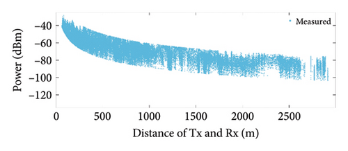
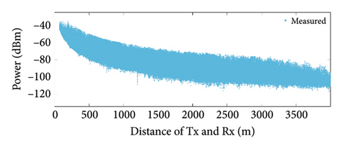
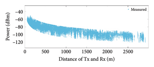
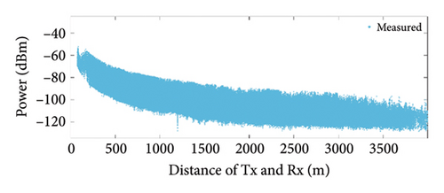
The measurement site comprehensively covers various typical environmental features in a macrocellular environment, with over 40,000 buildings including office buildings, residential communities, and shopping malls. As depicted in Figure 3, during the measurement activity, the Tx is placed at the designated position on the rooftop, while the Rx is positioned on top of the vehicle. The vehicle travels along the blue curve outlined in Figure 3. Receiver coordinates and received power are collected in real time as the vehicle moves. The measurement results are depicted in Figure 4. The minimum (MIN), maximum (MAX), average (AVG), and standard deviation (SD) of the measurement results under different conditions are presented in Table 2.

Table 2. The statistical results of the measurement outcomes.

Frequency (MHz)	LoS/NLoS	MIN (dBm)	MAX (dBm)	AVG (dBm)	SD (dBm)
900	LoS	−103.65	−28.61	−69.35	12.71
900	NLoS	−119.32	−36.00	−87.58	11.72

3500	LoS	−120.70	−51.17	−86.75	12.90
3500	NLoS	−128.70	−52.49	−104.74	10.97

From Figure 4 and Table 2, it can be observed that the average received power at 3500 MHz is lower compared with that at 900 MHz. This is due to the increase in propagation loss with frequency. In comparison to LoS, the average received power is lower in NLoS due to the longer propagation delay and energy loss during processes such as reflection and diffraction. The standard deviation of the measurement data under different frequencies and distances over a prolonged period remains stable at 10–13 dBm, indicating good stability of the measurement equipment for this test. In addition, the results also suggest that factors such as noise (moving individuals, vehicles, wind speed in the air, swaying trees, etc.) and equipment sensitivity in a macrocellular environment may have an impact ranging from −6 to 6 dBm.

2.2. Parameter Optimization and Numerical Analysis

According to the construction principle of BTM–SVR, the prediction efficiency and prediction accuracy of BTM–SVR are not only affected by the training samples but also mainly affected by α_b and the number of support vectors. This section first studies the impact of α_b on BTM–SVR and then studies the influence of the number of support vectors on BTM–SVR. Based on the comparative analysis with measurement results, the simulation of kilometer-level coverage prediction in macrocell is finally realized by combining the general scene BTM feature extraction algorithm and BTM–SVR.

2.2.1. Effect of α_b on BTM–SVR

The number of support vectors is set to 200, with a maximum iteration count of 100. The expected performance is RMSE < 3, and the values of α_b range from 0.001 to 1 in increments of 0.001. The simulation results are presented in Figure 5.

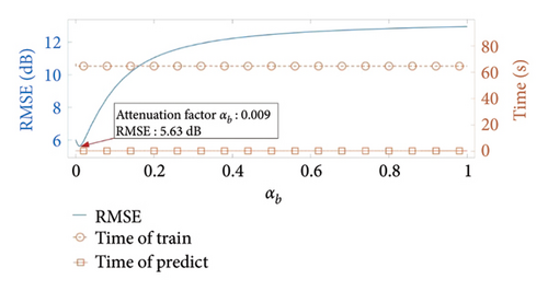
From Figure 5, it can be observed that when α_b < 0.009, the prediction accuracy of BTM–SVR increases with the increase of α_b. When α_b = 0.009, the prediction accuracy of BTM–SVR reaches its peak, with an RMSE of 5.63 dB. However, when α_b > 0.009, the prediction accuracy of BTM–SVR decreases as α_b increases. This phenomenon can be attributed to the fact that the predicted received power by BTM decreases linearly with increasing α_b, leading to corresponding changes in the “discrete process” of sample features mapped in a high-dimensional space by BTM. In addition, the variations in α_b have no impact on the computational efficiency of BTM–SVR during both the training and prediction processes.

2.2.2. Effect of the Number of Support Vectors on BTM–SVR

Set the maximum iteration number to 100, with an expected performance of RMSE < 3. The value of α_b is 0.009, and the support vector count ranges from 5 to 2000 in increments of 5. The results of the simulation are illustrated in Figure 6.

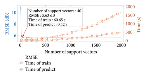
From Figure 6, it can be observed that when the number of support vectors is less than 40, the prediction accuracy of BTM–SVR increases with an increase in the number of support vectors. When the number of support vectors exceeds 40, BTM–SVR exhibits high prediction accuracy, with RMSE less than 6 dB and a tendency to stabilize. The training time and prediction time both increase with the increasing number of support vectors. This is due to the fact that the number of support vectors directly impacts the parameter count of BTM–SVR, including the size of matrices computed by the kernel function and the number of Lagrange multipliers. The increase in support vector count requires exponentially growing computational power.

2.2.3. Comparison and Analysis of Simulation Results With Measured Data

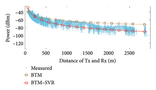
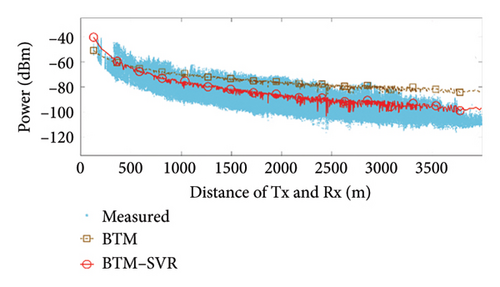
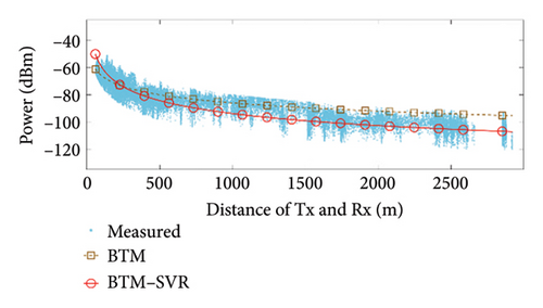
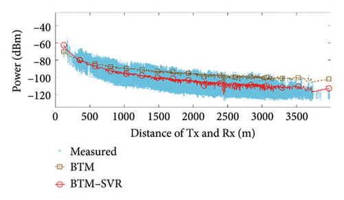
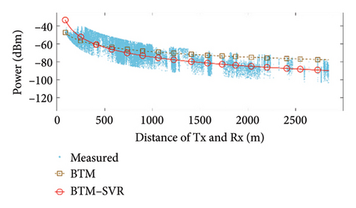
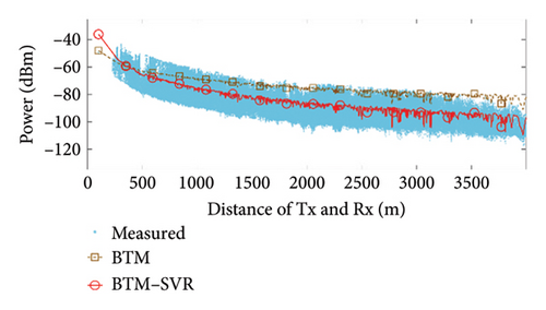
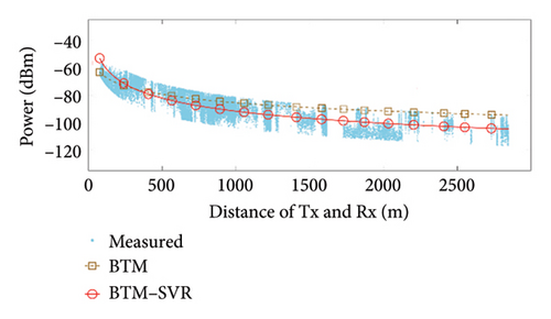
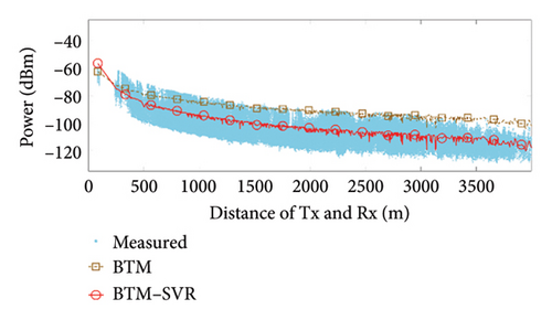
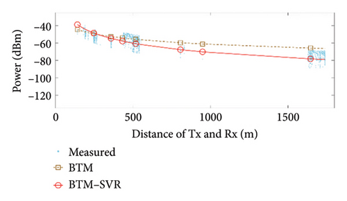
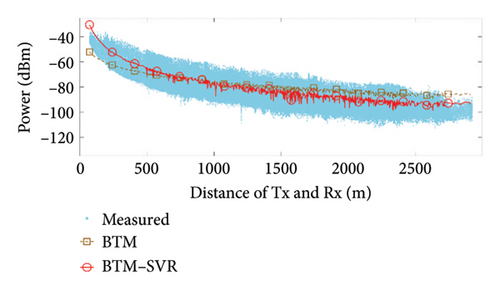
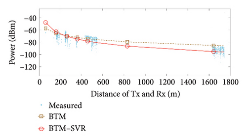
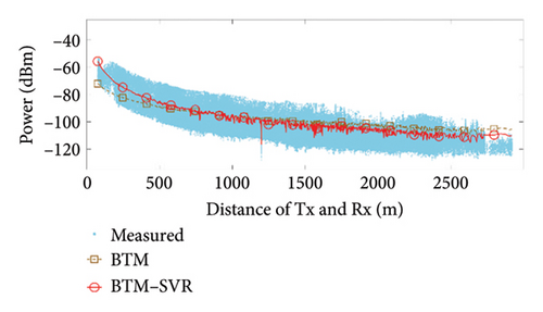
When α_b = 0.009 and the number of support vectors is 40, the predicted results of BTM and BTM–SVR under various conditions are compared with the measured results, as illustrated in Figure 7. The specific simulation results and RMSE values from measurements are presented in Table 3.

Table 3. RMSE values of BTM and BTM–SVR simulation results and measured results under different conditions.

Simulation scene	Frequency (MHz)	LoS/NLoS	BTM (dB)	BTM–SVR (dB)
SC # 1	900	LoS	11.65	6.13
	900	NLoS	14.72	6.61
	3500	LoS	7.73	5.85
	3500	NLoS	12.34	6.26

SC # 2	900	LoS	7.81	6.68
	900	NLoS	15.16	6.83
	3500	LoS	7.56	5.92
	3500	NLoS	15.64	6.76

SC # 3	900	LoS	7.35	5.83
	900	NLoS	9.43	6.98
	3500	LoS	7.04	5.68
	3500	NLoS	8.72	7.04

From the results shown in Figure 7 and Table 3, it can be seen that compared with BTM, the RMSE in the LoS condition at 900 MHz frequency was improved by 5.52 dB, 1.13 dB, and 1.52 dB in the three scenarios, respectively. The RMSE in the NLoS condition was improved by 8.11 dB, 8.33 dB, and 2.45 dB in the three scenarios, respectively. At 3500 MHz frequency, the RMSE in the LoS condition was improved by 1.88 dB, 1.64 dB, and 1.36 dB in the three scenarios, respectively. The RMSE in the NLoS condition was improved by 6.08 dB, 8.88 dB, and 1.68 dB in the three scenarios, respectively. Clearly, BTM–SVR addresses the issue of decreasing prediction accuracy in BTM as distance and the number of buildings passed increase. In various frequencies and scenarios, BTM–SVR outperforms BTM in both LoS and NLoS conditions, with a particularly notable improvement under NLoS conditions. The prediction accuracy of BTM–SVR is approximately 6.5 dBm, which closely aligns with the measured results.

2.2.4. Prediction of Coverage Area

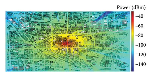
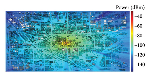
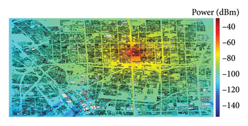
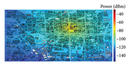
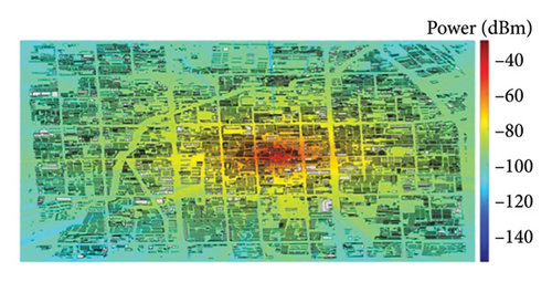
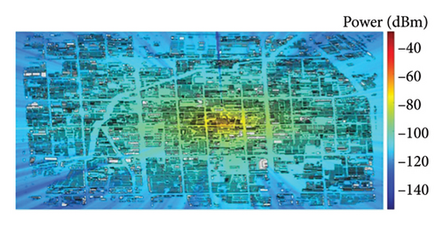
In network planning and optimization, it is often necessary to make predictions about regional coverage. BTM–SVR is capable of computing the received power by utilizing the extracted BTM feature information. Therefore, integrating the algorithm for extracting BTM feature information with BTM–SVR enables the construction of a coverage prediction simulation for macrocell. When α_b = 0.009 and the number of support vectors is 40, with a simulation granularity of 10 m, the coverage prediction results of BTM–SVR under different conditions are shown in Figure 8. The statistical results of the simulation calculations on the laptop with a CPU of i7-13700H are presented in Table 4.

Table 4. Statistical summary of simulation results under various conditions.

Simulation conditions	The number of buildings	Simulation scene dimensions (m)	Number of receivers	Simulation time-consuming (s)	Average computation time for Rx (ms)
(a) SC # 1, 900 MHz	15,464	6401^∗6198	417,852	3729	8.92
(b) SC # 1, 3500 MHz	15,464	6401^∗6198	417,852	3843	9.20

(c) SC # 2, 900 MHz	17,501	6159^∗5476	356,448	3361	9.43
(d) SC # 2, 3500 MHz	17,501	6159^∗5476	356,448	3482	9.77

(e) SC # 3, 900 MHz	10,815	4057^∗5348	232,522	1565	6.73
(f) SC # 3, 3500 MHz	10,815	4057^∗5348	232,522	1685	7.25

From Figure 8 and Table 4, it is evident that BTM–SVR supports kilometer-level surface coverage prediction, with the average computation time for individual receiver predictions being only a few milliseconds. Compared with 3500 MHz, the effective radiation range of 900 MHz is broader in scope. The greater the number of buildings within the coverage area, the lower the calculation efficiency, due to the decreased computational efficiency in feature extraction by BTM. Furthermore, the coverage prediction map computed by BTM–SVR shows clear linear stripes, which is due to the fact that BTM only considers the influence of electromagnetic waves on the Tx and Rx located on a straight line.

3. Conclusions

This paper proposes a machine learning method, BTM–SVR, for predicting wireless channels. The kernel function of BTM–SVR is inspired by BTM and is suitable for wireless channel prediction in macrocellular environments. Compared with the measured results, the RMSE of BTM–SVR at 900 MHz frequency in the LoS condition in the three scenes was 6.13 dB, 6.68 dB, and 5.83 dB, respectively. The RMSE in the NLoS condition was 6.61 dB, 6.83 dB, and 6.98 dB, respectively. At 3500 MHz frequency, the RMSE in the LoS condition in the three scenes was 5.85 dB, 5.92 dB, and 5.68 dB, respectively. The RMSE in the NLoS condition was 6.26 dB, 6.76 dB, and 7.04 dB, respectively. In addition, BTM–SVR exhibits highly efficient training and prediction speeds, making it well suited for large-scale coverage prediction simulations. This capability can significantly aid in network planning and optimization decision-making within macrocell environments.

Looking ahead, as the coverage area and distance increase, further measurements will be needed to systematically verify and enhance the model’s prediction accuracy. Meanwhile, to improve the applicability of our model, we plan to conduct further research and validation by fully considering diffraction and scattering factors in different urban environments in the future.

Conflicts of Interest

The authors declare no conflicts of interest.

Funding

This work was supported in part by the National Key Laboratory Fund of Electromagnetic Environment (Grant no. JCKY2024210C61424030301), the key project of Social Governance and Scientific and Technological Support for Smart Society (Grant no. 2022YFC3301403), and the Foundation of China Information Technology Designing & Consulting Institute Co. Ltd.

Acknowledgments

Open Research

Data Availability Statement

The data used to support the findings of this study are available from the corresponding author upon reasonable request.

References

1 Zhang P., Yang B., Yi C., Wang H., and You X., Measurement-based 5G Millimeter-Wave Propagation Characterization in Vegetated Suburban Macrocell Environments, IEEE Transactions on Antennas and Propagation. (2020) 68, no. 7, 5556–5567, https://doi.org/10.1109/tap.2020.2975365.
10.1109/TAP.2020.2975365
Web of Science® Google Scholar
2 Huang J., Liu Y., Wang C. X., Sun J., and Xiao H. L., 5G Millimeter Wave Channel Sounders, Measurements, and Models: Recent Developments and Future Challenges, IEEE Communications Magazine. (2019) 57, no. 1, 138–145, https://doi.org/10.1109/mcom.2018.1701263, 2-s2.0-85058076979.
10.1109/mcom.2018.1701263
Web of Science® Google Scholar
3 Wang X., Kong L., Kong F., Qiu F., Xia M., Arnon S., and Chen G., Millimeter Wave Communication: A Comprehensive Sur-Vey, IEEE Communications Surveys and Tutorials. (2018) 20, no. 3, 1616–1653, https://doi.org/10.1109/comst.2018.2844322, 2-s2.0-85048170119.
10.1109/comst.2018.2844322
Google Scholar
4 Jameel F., Wyne S., Nawaz S. J., and Chang Z., Propagation Channels for mmWave Vehicular Communications: State-of-the-Art and Future Research Directions, IEEE Wireless Communications. (2019) 26, no. 1, 144–150, https://doi.org/10.1109/mwc.2018.1800174, 2-s2.0-85059392379.
10.1109/mwc.2018.1800174
Web of Science® Google Scholar
5 Paran K. and Noori N., Tuning of the Propagation Model ITU-R P.1546 Recommendation, Progress in Electromagnetics Research B. (2008) 8, no. 5, 243–255, https://doi.org/10.2528/pierb08062201.
10.2528/pierb08062201
Google Scholar
6 Jaeckel S., Raschkowski L., Borner K., and Thiele L., QuaDRiGa: A 3-D Multi-Cell Channel Model With Time Evolution for Enabling Virtual Field Trials, IEEE Transactions on Antennas and Propagation. (2014) 62, no. 6, 3242–3256, https://doi.org/10.1109/tap.2014.2310220, 2-s2.0-84901992649.
10.1109/TAP.2014.2310220
Web of Science® Google Scholar
7 Ikegami F., Yoshida S., Takeuchi T., and Umehira M., Propagation Factors Controlling Mean Field Strength on Urban Streets, IEEE Transactions on Antennas and Propagation. (1984) 32, no. 8, 822–829, https://doi.org/10.1109/tap.1984.1143419, 2-s2.0-0021479001.
10.1109/TAP.1984.1143419
Web of Science® Google Scholar
8 Grubisic S., Carpes W. P., and Bastos J. P. A., Optimization Model for Antenna Positioning in Indoor Environments Using 2-D Ray-Tracing Technique Associated to a Real-Coded Genetic Algorithm, IEEE Transactions on Magnetics. (2009) 45, no. 3, 1626–1629, https://doi.org/10.1109/tmag.2009.2012760, 2-s2.0-61449180349.
10.1109/tmag.2009.2012760
Web of Science® Google Scholar
9 Papkelis E. G., Psarros I., Ouranos I. Ch. et al., A Radio-Coverage Prediction Model in Wireless Communication Systems Based on Physical Optics and the Physical Theory of Diffraction [Wireless Corner], IEEE Antennas and Propagation Magazine. (2007) 49, no. 2, 156–165, https://doi.org/10.1109/map.2007.376622, 2-s2.0-50249128207.
10.1109/map.2007.376622
Google Scholar
10 Hata M., Empirical Formula for Propagation Loss in Land Mobile Radio Services, IEEE Transactions on Vehicular Technology. (1980) 29, no. 3, 317–325, https://doi.org/10.1109/t-vt.1980.23859, 2-s2.0-0019045740.
10.1109/T-VT.1980.23859
Web of Science® Google Scholar
11 Okumura Y., Ohmori E., Kawano T., and Fukuda K., Field Strength and Its Variability in VHF and UHF Land Mobile Radio Service, Review of the Electrical Communication Laboratories. (1968) 16, no. 1, 825–873.
Google Scholar
12 Jo J.-H., Ingram M. A., and Jayant N., Deterministic Angle Clustering in Rectangular Buildings Based on Ray-Tracing, IEEE Transactions on Communications. (2005) 53, no. 6, 1047–1052, https://doi.org/10.1109/tcomm.2005.849979, 2-s2.0-22144434108.
10.1109/tcomm.2005.849979
Web of Science® Google Scholar
13 Zhao X. W., Fu Z. H., Fan W. et al., Semi-Deterministic Dynamic Millimeter-Wave Channel Modeling Based on an Optimal Neural Network Approach, IEEE Transactions on Antennas and Propagation. (2022) 70, no. 6, 4082–4095, https://doi.org/10.1109/tap.2022.3145438.
10.1109/tap.2022.3145438
Web of Science® Google Scholar
14 Tian L., Esposti V. D., Vitucci E. M., and Yin X., Semi-Deterministic Radio Channel Modeling Based on Graph Theory and Ray-Tracing, IEEE Transactions on Antennas and Propagation. (2016) 64, no. 6, 2475–2486.
10.1109/TAP.2016.2546950
Web of Science® Google Scholar
15 Smith D. P., Messier G. G., and Wasson M. W., Boreal Forest Low Antenna Height Propagation Measurements, IEEE Transactions on Antennas and Propagation. (2016) 64, no. 9, 4004–4011, https://doi.org/10.1109/tap.2016.2583490, 2-s2.0-84987681444.
10.1109/TAP.2016.2583490
Web of Science® Google Scholar
16 Olasupo T. O., Otero C. E., Olasupo K. O., and Kostanic I., Empirical Path Loss Models for Wireless Sensor Network Deploy-Ments in Short and Tall Natural Grass Environments, IEEE Transactions on Antennas and Propagation. (2016) 64, no. 9, 1–4021, https://doi.org/10.1109/tap.2016.2583507, 2-s2.0-84987660300.
10.1109/tap.2016.2583507
Google Scholar
17 Rashid A. K. and Zhang Q., An Efficient Method of Moments for Thick-Wire Antennas, IEEE Transactions on Antennas and Propagation. (2022) 70, no. 12, 12399–12404, https://doi.org/10.1109/tap.2022.3209277.
10.1109/tap.2022.3209277
Web of Science® Google Scholar
18 Echeveste J. I., De Aza M. A. G., and Zapata J., Shaped Beam Synthesis of Real Antenna Arrays via Finite-Element Method, Floquet Modal Analysis, and Convex Programming, IEEE Transactions on Antennas and Propagation. (2016) 64, no. 4, 1279–1286.
10.1109/TAP.2016.2526038
Web of Science® Google Scholar
19 Kong Y. D., Chen X. L., and Chu Q. X., Analysis of Stability and Numerical Dispersion of 3-D HIE-FDTD Method Including Lumped Elements, IEEE Transactions on Antennas and Propagation. (2023) 71, no. 10, 8130–8142, https://doi.org/10.1109/tap.2023.3302510.
10.1109/tap.2023.3302510
Google Scholar
20 Sotiroudis S. P., Goudos S. K., and Siakavara K., Deep Learning for Radio Propagation: Using Image-Driven Regression to Estimate Path Loss in Urban Areas, ICT Express. (2020) 6, no. 3, 160–165, https://doi.org/10.1016/j.icte.2020.04.008.
10.1016/j.icte.2020.04.008
Web of Science® Google Scholar
21 Zhang X., Shu X., Zhang B., Ren J., Zhou L., and Chen X., Cellular Network Radio Propagation Modeling With Deep Convo-Lutional Neural Networks, Proceedings of the 26th ACM SIGKDD International Conference on Knowledge Discovery & Data Mining, 2020, Virtual Event, 6–10.
Google Scholar
22 Ayadi M., Ben Zineb A., and Tabbane S., A UHF Path Loss Model Using Learning Machine for Heterogeneous Networks, IEEE Transactions on Antennas and Propagation. (2017) 65, no. 7, 3675–3683, https://doi.org/10.1109/tap.2017.2705112, 2-s2.0-85029620466.
10.1109/TAP.2017.2705112
Web of Science® Google Scholar
23 Wu L., He D., Ai B., Wang J., Liu D., and Zhu F., Enhanced Path Loss Model by Image-Based Environmental Characterization, IEEE Antennas and Wireless Propagation Letters. (2022) 21, no. 5, 903–907, https://doi.org/10.1109/lawp.2022.3151492.
10.1109/lawp.2022.3151492
Web of Science® Google Scholar
24 Sung S., Choi W., Kim H., and Jung J.-I., Deep Learning-Based Path Loss Prediction for Fifth-Generation New Radio Vehicle Communications, IEEE Access. (2023) 11, no. 1, 75295–75310, https://doi.org/10.1109/access.2023.3297215.
10.1109/access.2023.3297215
Web of Science® Google Scholar
25 Zhang Y., Wen J., Yang G., He Z., and Wang J., Path Loss Prediction Based on Machine Learning: Principle, Method, and Data Expansion, Applied Sciences. (2019) 9, no. 9, https://doi.org/10.3390/app9091908, 2-s2.0-85067190847.
10.3390/app9091908
Google Scholar
26 de Jong Y. L. C., Koelen M. H. J. L., and Herben M. H. A. J., A Building-Transmission Model for Improved Propagation Pre-Diction in Urban Microcells, IEEE Transactions on Vehicular Technology. (2004) 53, no. 2, 490–502, https://doi.org/10.1109/tvt.2004.823491, 2-s2.0-1942453378.
10.1109/tvt.2004.823491
Google Scholar
27 Nechayev Y. I. and Constantinou C. C., Statistical Modelling of Building Transmission in a Cellular Urban Environment, IET Microwaves, Antennas and Propagation. (2007) 1, no. 2, 355–362, https://doi.org/10.1049/iet-map:20050128, 2-s2.0-77955244520.
10.1049/iet-map:20050128
Web of Science® Google Scholar
28 Soni S. and Bhattacharya A., An Analytical Characterization of Transmission Through a Building for Deterministic Propaga-Tion Modeling, Microwave and Optical Technology Letters. (2011) 53, no. 8, 1875–1879, https://doi.org/10.1002/mop.26152, 2-s2.0-79960696493.
10.1002/mop.26152
Web of Science® Google Scholar
29 Gonsioroski L. H. and da Silva Mello L., Measurements of Building Transmission Loss and Delay Spread at 2.5 GHz, International Journal of Antennas and Propagation. (2015) 1.
Google Scholar
30 Prado D. R., López-Fernández J. A., Arrebola M., and Goussetis G., On the Use of the Angle of Incidence in Support Vector Regression Surrogate Models for Practical Reflectarray Design, IEEE Transactions on Antennas and Propagation. (2021) 69, no. 3, 1787–1792.
10.1109/TAP.2020.3015707
Web of Science® Google Scholar
31 Prado D. R., López-Fernández J. A., and Arrebola M., Support Vector Regression Models of Reflectarray Unit Cell in a Geomet-Rical 4-D Parallelotope Domain Around a Rectangle of Stability, IEEE Transactions on Antennas and Propagation. (2023) 71, no. 6, 5089–5099.
10.1109/TAP.2023.3266502
Google Scholar
32 Prado D. R., Naseri P., López-Fernández J. A., Hum S. V., and Arrebola M., Support Vector Regression-Enabled Optimization Strategy of Dual Circularly-Polarized Shaped-Beam Reflectarray With Improved Cross-Polarization Performance, IEEE Transactions on Antennas and Propagation. (2023) 71, no. 1, 497–507.
10.1109/TAP.2022.3215859
Web of Science® Google Scholar
33 Wang J., Wu Z., Hao Y., Yang C., and Shi Y., An SVR-Based Radio Propagation Prediction Model for Terrestrial FM Broad-Casting Services in beijing and Its Surrounding Area, IEEE Transactions on Broadcasting. (2024) 70, no. 1, 123–134, https://doi.org/10.1109/tbc.2023.3311335.
10.1109/tbc.2023.3311335
Google Scholar
34 Leonor N. R., Faria S., Ramos G. et al., Site-Specific Radio Propagation Model for Macrocell Coverage at Sub-6 GHz Frequencies, IEEE Transactions on Antennas and Propagation. (2022) 70, no. 10, 9706–9715, https://doi.org/10.1109/tap.2022.3184416.
10.1109/TAP.2022.3184416
Web of Science® Google Scholar

All articles

Research on the Macrocell Wireless Channel Model Based on Physic-Inspired Support Vector Regression Algorithm Wireless Channel Model in Macrocell Environment

Abstract