The finite element method was used in this study to explore the impact of surface roughness and thermal characteristics on slider bearings with non-Newtonian power-law fluid flow lubricant. One-dimensional transverse and longitudinal surface roughness models were considered under the stochastic assumption that roughness has a Gaussian random distribution. For improved computing efficiency, the surface’s uneven texture is transformed into a regular domain. For non-Newtonian power-law lubrication, a modified Reynolds equation was developed. The pressure distribution of the combined effect is less than that of the surface roughness and thermal effect in longitudinal surface roughness for all non-Newtonian parameters n and M^⊛ values. As a result, there is an 1.6% reduction in load-carrying capacity performance and negligible friction force for nonparallel w = 0.4 between the thermal effect and surface roughness. Nevertheless, for all non-Newtonian parameters n and M^⊛ values, the pressure distribution of the thermal effect in the transverse roughness model is smaller than that of the combined and surface roughness effects. Consequently, there is an 8.9% reduction in load-carrying capacity performance and a negligible friction force for nonparallel w = 0.4 between the surface roughness effect and the thermal effect condition, respectively. Additionally, the combined impacts at different temperatures were examined. As a result, in longitudinal models, the load-carrying capacity performance is better when the slider temperature is higher than the pad temperature, and vice versa for transverse models. Surface roughness and non-Newtonian power-law fluid characteristics generally enhance the performance of a slider bearing. Tables and graphs were employed to present the results.

1. Introduction

One of the most popular features of some types of machinery components is the slider bearing, which reduces friction between any two moving parts. The performance of plane slider bearings is largely dependent on the properties of the fluid, particularly if the fluid is non-Newtonian. The complex fluid viscosity of non-Newtonian fluids is dependent on factors such as temperature and shear rate; however, surface roughness can have a significant effect on the bearing’s performance as well as the flow of fluid; furthermore, the friction and wear of a bearing can be greatly influenced by its surface roughness, which may have an effect on the bearing’s overall performance and lifespan.

Special difficulties occur in non-Newtonian fluid flow applications with plane slider bearing. By aiding in the design of the bearings and optimizing these fluid-using devices, these findings may enhance the functionality and efficiency of machinery and equipment utilized in the biomedical engineering, materials processing, and oil and gas sectors.

In order to construct the Reynolds equation for the general lubrication problem of the non-Newtonian fluid, Yang et al. [1] treat the lubricant flow as the superposition of the Poiseuille flow and the Couette flow. Lin [2] conducted a theoretical investigation to examine the non-Newtonian effects of an isothermal, incompressible laminar-flow lubricant on the damping properties and dynamic stiffness of one-dimensional (1D) slider bearings. The modified Reynolds equation for bearing-squeeze action is derived from the Rabinowitsch fluid (cubic equation) model in order to take into consideration the non-Newtonian characteristics of lubricants as well as the slider’s transient motion. The effect of partial and full texturing on a hybrid thrust pad bearing with a non-Newtonian lubricant is theoretically examined by Yadav and Sharama [3]. The finite element method (FEM) with Reynolds boundary conditions was used to complete the task by Rao and Agarwal [4] which looked at the modified Reynold equation model that was lubricated with micropolar fluid. The modified Reynolds equation, applicable to power-law lubricants, was derived using an analytical approach for the analysis of slider bearings with non-Newtonian lubricants [5].

The static and dynamic performance of an orifice-compensated hole-entry hybrid journal bearing system taking into account the combined influence of surface roughness and non-Newtonian behavior of the lubricant is described in Nagaraju et al. [6]. The lubricant flow field in the clearance space of a rough journal bearing system has been solved using the modified form of the average Reynolds equation. The power-law model has been expected to be followed by non-Newtonian lubricants [7]. The treatment of a non-Newtonian lubricant’s flow in a slider bearing is dealt with analytically. Oladeinde et al. [8] investigated numerically the performance of a fixed inclined slider bearing whose surfaces are lubricated by a non-Newtonian power-law lubricant. Walters et al. [9] discuss the importance of non-Newtonian effects in journal bearing lubrication using a numerical approach. The modified Reynolds equation for non-Newtonian fluid with the rheological model in the frequency domain for journal bearing was derived by Haosheng and Darong [10].

Among the studies on the impact of surface roughness on various bearing types are those on hydrostatic bearings by Lin [11], journal bearings by Guha [12], and slider bearings by Christensen and Tonder [13]. Alternatively, Kumar [14] examined a segregated FEM of the Petrov–Galerkin framework with appropriate weight functions for a nonisothermal flow in the model’s high-speed slider bearings that has temperature-dependent viscosity and density. In Rathish Kumar and Srinivasa Rao [15], the load-carrying support’s slider bearing was numerically simulated using the FEM. Sinha and Adamu [16] conducted a thermohydrodynamic analysis of an infinitely many long tilted pad slider bearings with roughness using the finite difference method (FDM). In Adamu and Sinha [17], surface roughness is taken to be Gaussian randomly distributed and stochastic characteristic and heat conduction through both the pad and slider is taken into consideration for both of the two models of 1D transverse and longitudinal roughness.

Using the FEM, the authors of [18–20] recently examined the performance of the slider bearings in relation to surface roughness and temperature on 1D transverse and longitudinal roughness types. The static and dynamic properties of a few rough, porous Rayleigh step bearings lubricated with stress fluid were investigated by Naduvinamani and Angadi [21]. Nb and Angadi [22] examined how roughness and micropolar fluid affected the dynamic properties of inclined porous slider bearings. Gu et al. [23] investigated the static properties of aerostatics porous journal bearings using theoretical and numerical analysis. Transient elastohydrodynamic lubrication under line contact stiffness and damping behaviors were covered by Fang et al. [24]. Jamshed et al. [25] demonstrated how unsteady hybrid nanofluids can increase thermal efficiency in solar-powered aircraft using a single-phase optimized entropy analysis. Raees et al. [26] studied the energy transfer in a power-law nanofluid driven by magnetization to flow along a horizontal wall. Overall, our review of the literature and our knowledge gaps show that, when it comes to the derivation of the modified Reynold equation, FEM has not been shown to be able to solve the performance of the slider bearings over combined surface roughness and thermal effects with non-Newtonian fluid type. It is this that spurs us on to this study.

However, the derivation of the modified Reynolds equation for surface roughness (for 1D longitudinal and transverse) with thermal effect for slider bearing for non-Newtonian fluid flow type and solved by FEM has received little attention. Thus, the combined effect of temperature and surface roughness on a slider bearing with a non-Newtonian fluid film type by considering the local power-law exponent and consistency factor effect will be numerically analyzed using FEM in this paper.

2. Basic Equations

Figure 1 depicts the geometry and configuration of a rough, long slider bearing with a bearing length that is infinitely long compared to the fluid film’s thickness.

Details are in the caption following the image — **Figure 1**
Open in figure viewer PowerPoint

Geometry of one-dimensional roughness slider bearing.

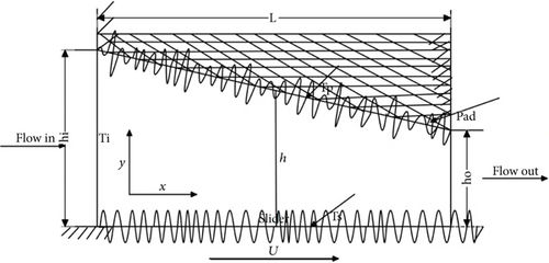
The developed equations to express the flow of lubricants in bearings result from simplifications of the governing equations of fluid flow. Dien and Elrod [27] adopted perturbation procedure to develop a generalized Reynolds equation for power-law fluids. With the usual assumptions made for the derivation of the Reynolds equation, the simplified momentum equations are written as given in Desu Tessema et al. [18].

Equations of momentum and continuity, respectively,

(1)

(2)

The viscosity μ is dependent on the second invariant of the strain rate tensor which reduces to

(3)

where I is the second invariant of the strain rate tensor, n is the local power-law exponent, and m is the consistency factor. The detailed explanation of the non-Newtonian power-law Reynolds equation and its derivation is given in Ghosh et al. [28]. Thus, the generalized Reynolds equation is determined as follows:

*
The fluid is a non-Newtonian lubricant.
*
The fluid film thickness is significantly less than other bearing dimensions.
*
The inertia and body force of the fluid are negligible.
*
The lubricant is laminar and incompressible.
*
There is no slip at the bearing surfaces of fluid flow.

Based on the above assumptions, using the boundary conditions u = U, v = 0 on the slider and u = v = 0 on the pad, combine Equations (1), (2), and (3) to obtain the generalized power-law Reynolds equation for non-Newtonian. Substituting ρ with ρ_av yields the power-law’s generalized modified Reynolds equation, which is as follows:

(4)

where H_t is the thickness of the lubricant film, U is the velocity of the moving surface of the slider, and ρ_av is the average density of the slider bearing.

To arrive at the energy equation, the following assumptions are considered in addition to the lubrication assumption given above:

1.
Conduction terms are negligible other than those across the fluid film.
2.
Specific heat and thermal conductivity are constant.

The equation of energy becomes

(5)

Density is assumed to be temperature dependent and expressed by the following equations:

Based on the above assumptions, ρ₀ and ρ_av are the density at temperature T and ambient temperature T_a, respectively, λ is the coefficient of thermal expansion, the subscript a denotes an ambient condition, and T_av is the average temperature on the slider.

2.1. Basic Assumptions

Christensen [29], Sinha and Adamu [16], Zhu et al. [30], and Desu Tessema et al. [18] all detail the fundamental presumptions we made. This work uses two fundamental assumptions from Christensen [29] to handle 1D rough surface topography. The non-Newtonian lubrication model for power-law fluid, with its 1D longitudinal rough surface and 1D transverse rough surface, is based on three underlying assumptions: The direction perpendicular to the surface roughness direction is represented by s, and the direction parallel to the surface roughness direction is represented by k.

a.
It will be assumed that the stochastic variable ∂P/∂k has zero variance or that the deterministic variable, the pressure gradient in the roughness direction (∂p/∂k), exists.
b.
We will assume that the variable q_s, which represents the unit flow perpendicular to the direction of surface roughness, is deterministic, meaning that the variance of the stochastic variable q_s is zero.
c.
By Sinha and Adamu [16], the velocity and temperature assumptions were refined. The temperature and velocity magnitudes related to roughness are negligible when compared to the corresponding general bearing magnitudes. The gradients of temperature ∂T/∂y, velocity ∂u/∂y, and variances of ρ are therefore negligible in the direction of roughness.

Under the assumption c, the roughness-related magnitudes of ρ_av are small in comparison to the overall bearing magnitudes of ρ_av. The slider bearing 1D transverse and longitudinal roughness types are the two categories of 1D roughness models described in the theory. The degree of roughness in the surface’s sliding path is represented by long, narrow ridges and furrows, according to the 1D longitudinal roughness model (x-direction). As a result, the thickness of the film can be represented as a function of the form given in [29, 20, 16]

(6)

where h_t is the nominal (smooth) part, which measures the large-scale part of the film geometry, including any long wavelength disturbances, and δ is a randomly varying quantity with a zero mean, which arises due to the surface roughness measured from the nominal level.

In the transverse roughness model type, the thickness of the film can be described as a function of its form.

Taking the expected values on both sides of the Reynolds equation of power-law fluid, we obtained that

where E(s) is the expectancy operator and f(s) is the probability density distribution for the stochastic variables. Based on the aforementioned assumptions a and b, the non-Newtonian power-law Reynolds lubrication equation for 1D longitudinal roughness, the expectation values for the coefficient function are

(7)

As some of the details are expressed by Sinha and Adamu [16] and Zhu et al. [30], the derived non-Newtonian power-law Reynolds equation for 1D longitudinal roughness becomes

(8)

According to Sinha and Adamu [16], m, ∂u/∂y, ρ, u, and v are independent random variables. The expected value of Equations (1) and (2) becomes

(9)

(10)

The expected value for the energy equation

(11)

Using Zhu et al. [30] and the aforementioned assumptions a and b, the transverse roughness power-law Reynolds equation for non-Newtonian flow and the expectation values for some of the coefficient functions in transverse roughness are as follows:

(12)

(13)

(14)

The transverse roughness equations for momentum, continuity, and energy will resemble the longitudinal roughness model. One can approximate the unit heat flow in the slider direction to be of negligible variance since a unit flow is assumed to be of negligible variance. Consequently, the gradient of temperature in the slider direction turns into a random variable with very little variance. As a result, the form of the transverse roughness energy equation will be identical to that of the longitudinal roughness case. The following nondimensional variables, according to Sinha and Adamu [16] and Desu Tessema et al. [18], have been used:

The nondimensional expression for power-law non-Newtonian modified generalized Reynold’s equation found in (8) through (14) can be reformulated in the following ways for the longitudinal roughness model:

(15)

For the transverse roughness model, the modified power-law generalized non-Newtonian Reynolds equation is as follows:

(16)

(17)

(18)

(19)

where

Boundary conditions:

at x^⊛ = 0,

at x^⊛ = 1, u^⊛ = 1, v^⊛ = 0, on the slider, and u^⊛ = v^⊛ = 0 on the pad of the bearing. The following temperature boundary conditions are applied to the energy equation: T^⊛ = T^s on the slider, T^⊛ = T^p on the pad, and T^⊛ = Tⁱ at inlet (x^⊛ = 0), where

3. Transformation of the Problem

The irregular domain is converted to a regular geometric domain, as stated in Sinha and Adamu [16] and Desu Tessema et al. [18] to simplify the numerical computation. The following linear transformation Equation (20) was selected, assuming that the roughness on the pad and the roughness on the runner are the same random distributions (δ₁ = δ₂):

(20)

By using the above transformations, the governing Equations (15)–(19) become

(21)

(22)

(23)

(24)

(25)

where

The detail has been given in Sinha and Adamu [16].

The corresponding nondimensional density expressions in the new coordinate system are

(26)

where

The corresponding boundary conditions are

The nondimensional load-carrying capacity W^⊛ and the friction force F^⊛ are determined from the following equations, respectively:

(27)

4. Finite Element Formulation

Using bilinear rectangular elements which are provided in a similar manner in Desu Tessema et al. [18], one must first form the weighted integral Equations (21)–(25) and then apply integration by parts to the terms with second derivatives to derive the above equations’ weak form.

Let Ω be divided into N_e bilinear rectangular elements, and

where N_e is the number of rectangular elements, Ω_e denotes the interior domain of an element, and Γ_e is the boundary of Ω_e.

The resulting elemental weak form of Equations (21)–(25) is as follows:

(28)

(29)

(30)

(31)

(32)

where N_i is the weight function. To generalize the formulation, it is assumed that the same order of polynomials is used to approximate velocity, pressure, and temperature unknowns, that is,

(33)

where the shape (basis) functions ⋔_j that are used to build the approximate solution, U_j, V_j, P_j, and T_j are the nodal unknown values for velocity, pressure, and temperature, and nel is the number of nodal elements; for example, nel = 2 for P and nel = 4 for U, V, and T. The weight functions chosen for generalized finite element method (GFEM) consideration are identical to the shape functions (N_i = ⋔_j).

The weighted residual formulation of the above equation is obtained by replacing (28)–(32) with the approximation Equation (33), like that of Desu Tessema et al. [18]. As a result, the decoupled equations for U, V, and T, as well as the weak form of P, are displayed as follows:

(34)

(35)

(36)

(37)

(38)

4.1. Treatment of the Solution

FEM was developed and used to solve the system of equations with a finite number of unknowns. There are nonlinear terms in the formulated equations. Owing to this nonlinearity, a directive iterative approach is used to solve the algebraic system of equations, based on the general steps of solving the systems of equations which is given in the general algorithm (Section 4.2).

To the accuracy of tolerance (Tol), the approximate solution of the non-Newtonian fluid flow is obtained; the error is computed as

and φ_z are values of the unknown variables at nodal points.

The iteration was carried out with (Tol) = 10⁻³, 10⁻⁴, and 10⁻⁵. However, there is no significant difference in the approximation. The outcome was accomplished by developing MATLAB code for MATLAB Software Version 2021.

4.2. General Algorithm

The following algorithm is used to approximate the solution of all field variables.

Step 1. Initialization

i.
Input the constant data value: λ^⊛, β^⊛, σ^⊛, P_r, E, P_e, n, m^⊛.
ii.
Set boundary conditions for u^⊛, v^⊛, T^⊛, P^⊛.
iii.
Set fictitious values for u^⊛, v^⊛, T^⊛, P^⊛ over the entire grid points.

Step 2. Evaluate p^⊛new using Equation (34) or (35).

Step 3. Evaluate u^⊛new using p^⊛new, u^⊛old, v^⊛old, and T^⊛old and Equation (36).

Step 4. Evaluate v^⊛new using u^⊛new, v^⊛old, and T^⊛old and Equation (37).

Step 5. Evaluate T^⊛new using p^⊛new, u^⊛new, v^⊛new, and T^⊛old and Equation (38).

Step 6. Test for convergence.

Step 7. Repeat steps 2–6 till convergence is obtained on all field variables.

Step 8. Calculate load-carrying capacity W^⊛ and friction force F^⊛ using Equation (27).

5. Results and Discussion

The parameters of bearing in this article for non-Newtonian fluid types seem to be functions of w, n, m^⊛, and σ^⊛, in addition to the dimensionless parameters P_e and E. The parameter values chosen by the Lebeck consideration, as reported in Schumack [31], are as follows: μ_a = 0.0174 Pas, β = 0.035 K, λ = 0.0012 K, k = 0.132 W/(mK), U = 20 m/s, h_i = 0.00005 m, B = 0.1 m, c = 1,926 J/kgK, T_a = 310 K, ρ_a = 897.1 kg/m³. With fixed values for P_e, P_r, and E_c, the simulations took place for a variety of values for the parameters w, λ^⊛, β^⊛, σ^⊛, n, and m^⊛. The effects of texture can only be felt via h_o/3σ^⊛, where h_o is the minimum film thickness as established by Gururajan and Prakash [32]. When h_o ≫ 3σ^⊛, roughness has negligible impact. On the other hand, bearing performance may be significantly affected if h_o ≈ 3σ^⊛ (within the HD limit, that is, h_o > 3σ^⊛). The parameter roughness of σ^⊛ is taken to be fixed at 0.1 for comparison’s sake. For w = 0.4 and w = 1.0, respectively, this translates to 25% and 10% of the minimum film thickness. Moreover, it is assumed that the constants λ^⊛ = 0.4 and β^⊛ = 10 are fixed for the same.

The results of the temperature performance, drag force, load-bearing capacity, and pressure distribution have been studied. The solutions are shown using tables and graphs. To guarantee the grid independence of the results, the numerical simulations were performed using 10 by 10, 20 by 20, and 25 by 25 grid points on a variety of grid systems. The load-carrying capacity performance (LCCP) for different grids has been compared and shown in Table 1. This ultimately leads to the view that a grid-independent solution is produced by the 25 by 25 grid scheme.

Table 1. Performance of load-carrying capacity versus inclination on different grid systems for n = 0.95, M^⊛ = 0.53.

	w	0.4	0.5	0.6	0.7	0.8	0.9	1.0
25	W^⊛	0.2951	0.2071	0.1412	0.0907	0.0513	0.0202	0.0045
20	W^⊛	0.2947	0.2069	0.1412	0.0907	0.0513	0.0202	0.0045
10	W^⊛	0.2914	0.2054	0.1406	0.0906	0.0513	0.0202	0.0045

In the result that follows, emphasis has been given to the following conditions, which were considered in Desu Tessema et al. [18]:

a.
The combined effect of thermal and surface roughness
b.
Thermal effect on the smooth surface
c.
Pure surface roughness effect (with constant viscosity and density)

5.1. 1D Longitudinal Roughness

Figures 2, 3, and 4 show the 1D longitudinal distribution of pressure performance caused by surface roughness and the combined influence of temperature for non-Newtonian fluid flow for various values of local power-law exponent (n) and consistency factor (M^⊛). The LCCP is in increasing order of rising n value for any constant value of x^† and M^⊛. Similarly, LCCP is increasing as M^⊛ increases for the same value of n as we observe in the aforementioned figure. This demonstrates that, for a range of M^⊛ values, the bearing design will get better as n increases, taking into account the effects of thermal and surface roughness on LCCP. In addition, the consistency factor is also a critical parameter in the performance of slider bearings over non-Newtonian power-law fluids.

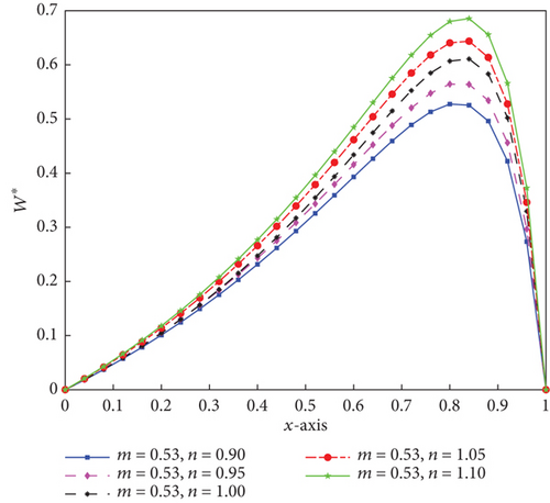
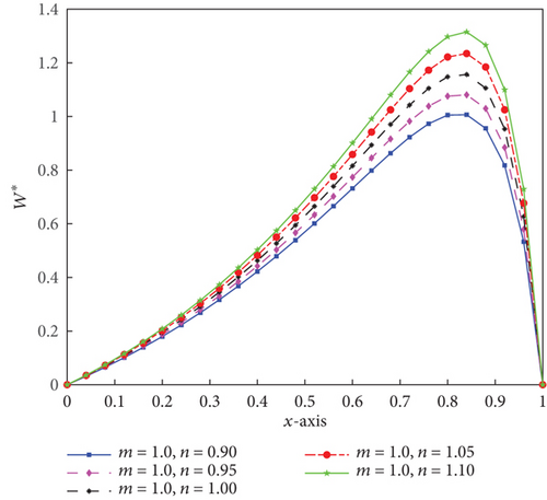
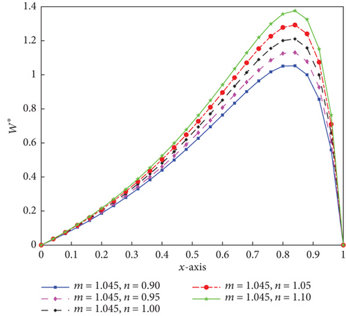
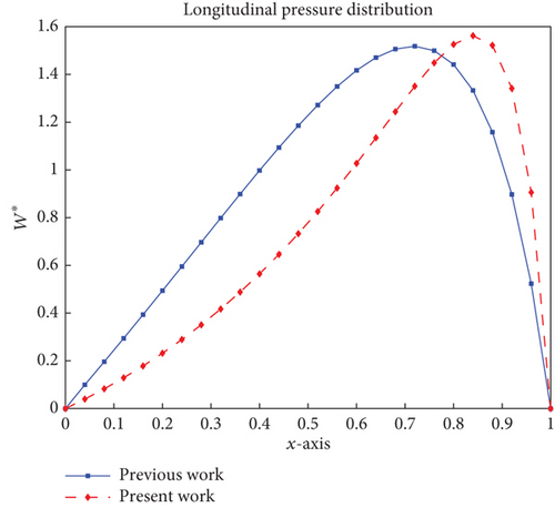
The pressure distributions for non-Newtonian fluid type of power-law for a plane slider bearing are in good agreement with Sinha and Adamu [16], Kumar [14], Rathish Kumar and Srinivasa Rao [15], and Desu Tessema et al. [18], which can be used as a cross-check to verify validity of the numerical method result. Furthermore, the pressure distribution peak can be seen nearer the outlet. Distribution of the pressure for non-Newtonian fluid type lubricant of power-law constant of a slider bearing for n = 1.1 and M^⊛ = 1.045, along with the pressure distribution for laminar Newtonian fluid type, performed in Desu Tessema et al. [18], is shown in Figure 5, demonstrating the superiority of the current work over previous work.

For the inclination parameter w = 0.4, the bearing performance of LCCP and drag force of 1D longitudinal roughness corresponding to the ahead of illnesses are shown in Table 2. It is clear that between conditions b and a, there is a decrement of nearly 1.6% in LCCP for all values of n and M^⊛ = 0.530. The drag frictional force between conditions a and b is also negligible for all values of n and M^⊛ = 0.530. Furthermore, as this table illustrates, under all conditions, the LCCP and drag force increase as the values of n and M^⊛ rise.

Table 2. Longitudinal roughness W^⊛ and F^⊛ at different values of n and M^⊛.

Condition	M^⊛	W^⊛	n
Condition	M^⊛	F^⊛	0.9000	0.9500	1.0000	1.0500	1.1000
a	0.530	W^⊛	0.2776	0.2951	0.3127	0.3306	0.3487
	0.530	F^⊛	1.5507	1.5510	1.5512	1.5514	1.5515
	1.000	W^⊛	0.5201	0.5528	0.5858	0.6193	0.6534
	1.000	F^⊛	1.5834	1.5842	1.5845	1.5846	1.5846
	1.045	W^⊛	0.5432	0.5772	0.6117	0.6467	0.6821
	1.045	F^⊛	1.5874	1.5881	1.5884	1.5884	1.5879

b	0.530	W^⊛	0.2820	0.2999	0.3179	0.3362	0.3549
	0.530	F^⊛	1.5502	1.5505	1.5506	1.5507	1.5507
	1.000	W^⊛	0.5285	0.5618	0.5956	0.6299	0.6646
	1.000	F^⊛	1.5818	1.5821	1.5822	1.5819	1.5813
	1.045	W^⊛	0.5519	0.5866	0.6220	0.6578	0.6938
	1.045	F^⊛	1.5853	1.5858	1.5858	1.5855	1.5846

c	0.530	W^⊛	0.2796	0.2971	0.3149	0.3329	0.3511
	0.530	F^⊛	1.5520	1.5525	1.5528	1.5532	1.5534
	1.000	W^⊛	0.5276	0.5607	0.5941	0.6281	0.6624
	1.000	F^⊛	1.5928	1.5943	1.5957	1.5968	1.5977
	1.045	W^⊛	0.5514	0.5859	0.6209	0.6563	0.6923
	1.045	F^⊛	1.5980	1.5997	1.6011	1.6024	1.6033

This is because, in this instance for the combined condition effect, the density of the fluid lubricant is decreased. As a result, the equivalent LCCP is reduced. Additionally, for all values of n and M^⊛ = 0.530, the LCCP between conditions b and c differs by 0.9%, and the change in drag force for the nonparallel (w = 0.4) is decreased by 0.14%. The surface roughness of plane slider bearing is assumed to have the characteristics of furrows, ridges of long narrow, and valleys in the flow direction (x-axis) for the 1D longitudinal surface texture model type in particular. This facilitates quick lubricant flow and lowers pressure distribution, which suggests a lower LCCP in comparison to other circumstances.

The drag force and LCCP performance of 1D longitudinal roughness corresponding to the above conditions are shown in Table 3 for various fluid gap parameters of non-Newtonian power-law fluid flow. The values of the pressure developed for each fixed n and M^⊛ are in the order of LCCP due to condition (a)< condition (c)< condition (b) for all circumstances, indicating that LCCP is in the same order as the corresponding condition of pressure. Condition (b)< condition (a)< condition (c) for all values n and M^⊛ over the whole inclination represent the order of the frictional force. This table shows that, under all conditions, the LCCP and drag force increase as n and M^⊛ rise and fall as the fluid gap decreases.

Table 3. Longitudinal roughness W^⊛ and F^⊛ for different values of n and M^⊛ versus inclination.

M^⊛	n	C_i	W^⊛	w
M^⊛	n	C_i	F^⊛	0.4	0.5	0.6	0.7	0.8	0.9	1.0
0.53	0.95	a	W^⊛	0.2951	0.2071	0.1412	0.0907	0.0513	0.0202	0.0045
		a	F^⊛	1.5510	1.3959	1.2791	1.1873	1.1130	1.0515	0.9997
		b	W^⊛	0.2999	0.2098	0.1429	0.0917	0.0518	0.0203	0.0045
		b	F^⊛	1.5505	1.3957	1.2789	1.1872	1.1130	1.0515	0.9997
		c	W^⊛	0.2971	0.2099	0.1447	0.0946	0.0555	0.0246	0.0000
		c	F^⊛	1.5525	1.3973	1.2803	1.1883	1.1138	1.0520	1.0000
	1.05	a	W^⊛	0.3306	0.2307	0.1566	0.1002	0.0564	0.0221	0.0050
		a	F^⊛	1.5514	1.3957	1.2786	1.1867	1.1126	1.0513	0.9997
		b	W^⊛	0.3362	0.2339	0.1585	0.1013	0.0570	0.0223	0.0050
		b	F^⊛	1.5507	1.3953	1.2784	1.1866	1.1125	1.0512	0.9997
		c	W^⊛	0.3329	0.2338	0.1605	0.1046	0.0612	0.0270	0.0000
		c	F^⊛	1.5532	1.3973	1.2799	1.1878	1.1134	1.0518	1.0000

1.0	0.95	a	W^⊛	0.5528	0.3855	0.2603	0.1642	0.0892	0.0302	0.0165
		a	F^⊛	1.5842	1.4045	1.2747	1.1774	1.1027	1.0443	0.9979
		b	W^⊛	0.5618	0.3907	0.2633	0.1659	0.0900	0.0304	0.0166
		b	F^⊛	1.5821	1.4034	1.2740	1.1770	1.1025	1.0442	0.9979
		c	W^⊛	0.5607	0.3960	0.2729	0.1785	0.1047	0.0464	0.0000
		c	F^⊛	1.5943	1.4137	1.2827	1.1840	1.1078	1.0479	1.0000
	1.05	a	W^⊛	0.6160	0.4271	0.2871	0.1803	0.0976	0.0328	0.0182
		a	F^⊛	1.5846	1.4029	1.2723	1.1751	1.1009	1.0433	0.9978
		b	W^⊛	0.6265	0.4331	0.2906	0.1823	0.0985	0.0331	0.0184
		b	F^⊛	1.5820	1.4015	1.2715	1.1746	1.1006	1.0431	0.9977
		c	W^⊛	0.6246	0.4389	0.3013	0.1964	0.1149	0.0508	0.0000
		c	F^⊛	1.5967	1.4137	1.2815	1.1825	1.1066	1.0472	1.0000

1.045	0.95	a	W^⊛	0.5772	0.4023	0.2714	0.1708	0.0924	0.0308	0.0180
		a	F^⊛	1.5881	1.4053	1.2738	1.1759	1.1012	1.0433	0.9976
		b	W^⊛	0.5866	0.4077	0.2745	0.1726	0.0933	0.0310	0.0182
		b	F^⊛	1.5858	1.4041	1.2731	1.1754	1.1010	1.0431	0.9976
		c	W^⊛	0.5859	0.4138	0.2852	0.1865	0.1094	0.0485	0.0000
		c	F^⊛	1.5997	1.4158	1.2830	1.1834	1.1070	1.0473	1.0000
	1.05	a	W^⊛	0.6467	0.4481	0.3008	0.1885	0.1016	0.0335	0.0200
		a	F^⊛	1.5884	1.4033	1.2710	1.1732	1.0991	1.0420	0.9974
		b	W^⊛	0.6578	0.4544	0.3044	0.1905	0.1025	0.0338	0.0202
		b	F^⊛	1.5855	1.4017	1.2701	1.1726	1.0988	1.0419	0.9974
		c	W^⊛	0.6563	0.4610	0.3164	0.2062	0.1206	0.0533	0.0000
		c	F^⊛	1.6024	1.4157	1.2816	1.1818	1.1056	1.0465	1.0000

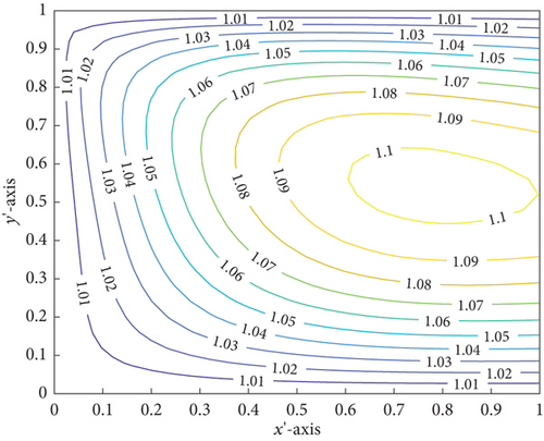
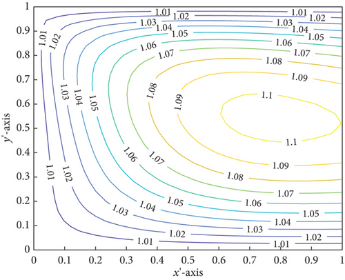
The LCCP that developed in the bearings in a and b relative to c when the bearing inclination parameter of w = 1 is caused by fluid expansion for varying values of n and M^⊛ as the lubricant temperature rises. The temperatures in Figures 6 and 7 do not significantly differ between a and b.

A suction action may happen in parallel plane slider bearings when the surface boundary temperature of the slider bearing is lower than the pad temperature, according to Zienkiewicz [33], which investigated pads and sliders of a plane slider bearing at different boundary temperatures. As a consequence, the LCCP can drastically drop.

Considering the boundary temperature of the slider and pad over the effect of thermal (T_p > T_s or T_p < T_s) on the LCCP and drag frictional force of a slider bearing is of enormously realistic relevance, according to Pinkus and Sternlicht [34]. He claims that based on his finding, in reality, the stationary surface of the slider is usually warmer than the moving part of slider surface. Another very important condition in a slider bearing application is taking into account the inlet lubricant boundary temperature being lower than the pad and slider boundary temperatures of the bearing. Based on different cases of temperature boundary conditions given, the combined effects have been considered for the non-Newtonian power-law fluid flow lubricant at the following temperature boundary conditions:

Case i: Tⁱ = T^p = 1.1 and T^s = 1.2.

Case ii: Tⁱ = T^s = 1.1 and T^p = 1.2.

Case iii: Tⁱ = 1.0, T^s = 1.1, and T^p = 1.2.

Case iv: Tⁱ = 1.0, T^s = 1.2, and T^p = 1.1.

Table 4 displays the drag force and LCCP of non-Newtonian fluid film lubricant of 1D longitudinal roughness for various n and M^⊛ power-law exponent effects corresponding to the aforementioned cases. The inflow inlet boundary temperature is lower than or equal to the other solid body of slider bearing. When the boundary temperature of the solid bodies are differs between Case i and Case ii for w = 0.4, the bearing performance of the pressure differs by 7%. For w = 1, however, Case ii performs somewhat better than Case i over all non-Newtonian constant consideration in terms of pressure and drag force. In the case of friction force, Cases ii and i are almost equal unless some differ from one another.

Table 4. Longitudinal roughness W^⊛ and F^⊛ for different values of n and M^⊛ and cases.

Case	n/M	W^⊛	w
Case	n/M	F^⊛	0.4	0.5	0.6	0.7	0.8	0.9	1.0
i	0.95/0.53	W^⊛	0.3065	0.2179	0.1510	0.1002	0.0601	0.0284	0.0031
	0.95/0.53	F^⊛	1.5516	1.3962	1.2790	1.1870	1.1125	1.0508	0.9989
	1.05/1.045	W^⊛	0.6725	0.4721	0.3231	0.2092	0.1206	0.0510	0.0040
	1.05/1.045	F^⊛	1.5905	1.4038	1.2703	1.1714	1.0965	1.0387	0.9936

ii	0.95/0.53	W^⊛	0.2839	0.1968	0.1319	0.0823	0.0437	0.0135	0.0104
	0.95/0.53	F^⊛	1.5509	1.3961	1.2795	1.1880	1.1138	1.0525	1.0007
	1.05/1.045	W^⊛	0.6214	0.4248	0.1693	0.1693	0.0844	0.0182	0.0335
	1.05/1.045	F^⊛	1.5876	1.4039	1.1759	1.1759	1.1026	1.0460	1.0017

iii	0.95/0.53	W^⊛	0.2920	0.2046	0.1395	0.0896	0.0509	0.0204	0.0037
	0.95/0.53	F^⊛	1.5513	1.3964	1.2796	1.1879	1.1136	1.0521	1.0002
	1.05/1.045	W^⊛	0.6399	0.4426	0.2967	0.1860	0.1005	0.0338	0.0184
	1.05/1.045	F^⊛	1.5898	1.4052	1.2733	1.1757	1.1016	1.0444	0.9995

iv	0.95/0.53	W^⊛	0.3068	0.2184	0.1523	0.1014	0.0616	0.0302	0.0052
	0.95/0.53	F^⊛	1.5522	1.3968	1.2796	1.1875	1.1130	1.0512	0.9992
	1.05/1.045	W^⊛	0.6732	0.4736	0.3254	0.2122	0.1243	0.0553	0.0008
	1.05/1.045	F^⊛	1.5934	1.4066	1.2729	1.1738	1.0985	1.0404	0.9948

This mentioned table demonstrates that if the inflow inlet boundary temperature is lower than the other two solid bodies of slider bearing, Case iii’s friction force and LCCP show lower performance than Case iv’s for each fluid gap parameter value. Due to these many numerous factors and others, if the stationary part of slider bearing temperature rises above the other solid part of slider bearing temperature, the temperature may rise over all the slider bearing body that could affect the bearing’s ability to support pressure and its drag force.

Generally, we observed that in each case given above, when the values of the non-Newtonian parameters n and M^⊛ increase, LCCP and drag force increase as well. In contrast to this, LCCP and frictional values decrease as the fluid gap parameter value decreases.

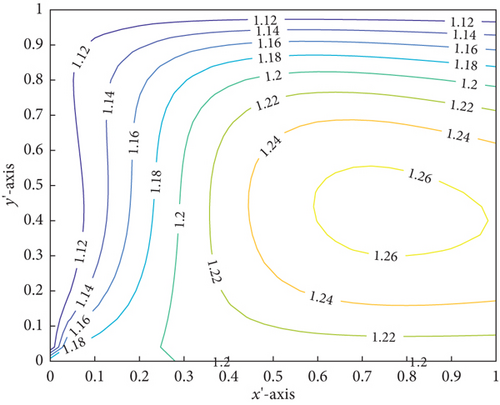
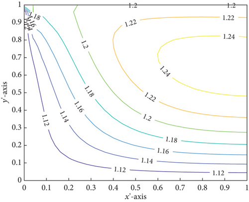
Figures 8 and 9 show the sliders over all temperature contours for Case i and Case ii for w = 0.4 to grasp more. Due to the fact that Case ii has more cumulative average temperature than Case i, Case ii’s LCCP for various values of n and M^⊛ of non-Newtonian power-law fluid lubricant is lower than that of Case i.

In Table 5, assuming that inflow inlet boundary pressure is equal to zero, the LCCP of 1D transversal and longitudinal surface texture for different values of σ^⊛, n = 0.95, and M^⊛ = 0.53 is displayed. For 1D longitudinal surface roughness of slider bearing to support LCCP, it is evident that non-Newtonian fluid lubricants with less surface texture σ^⊛ function show best results. For the 1D transverse surface texture model type, however, the opposite is true. Furthermore, as the surface texture value changes, there is a negligible variation in drag force for both types of models. As a consequence, a non-Newtonian fluid lubricant that has high surface texture values in the transverse model has greater effect thresholds, which is connected to its ability to hold more heavy loads.

Table 5. Effect of surface roughness on LCCP and drag force for different values of σ^⊛ at w = 0.4.

Type	σ^⊛	0.0	0.02	0.04	0.06	0.08	0.10
Longitudinal	w^⊛	0.2999	0.2997	0.2991	0.2981	0.2968	0.2951
Longitudinal	F^⊛	1.5505	1.5505	1.5505	1.5507	1.5508	1.5510
Transversal	w^⊛	0.2999	0.3009	0.3042	0.3096	0.3172	0.3272
Transversal	F^⊛	1.5505	1.5505	1.5504	1.5504	1.5503	1.5502

This is because the 1D longitudinal roughness model contains that the texture appears as furrows, long, narrow ridges, and valleys in the sliding direction (x-axis), allowing for the fast non-Newtonian fluid lubricant flow and resulting in a drop in pressure distribution, implying a reduction in LCCP. However, in the case of a transverse roughness pattern, which consists of valleys and ridges running in the direction perpendicular to sliding (x-direction), which obstruct the fluid flow lubricant, LCCP rises as a consequence.

5.2. Transverse 1D Roughness

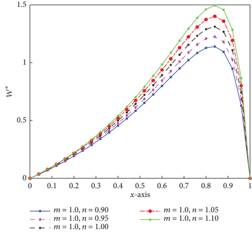
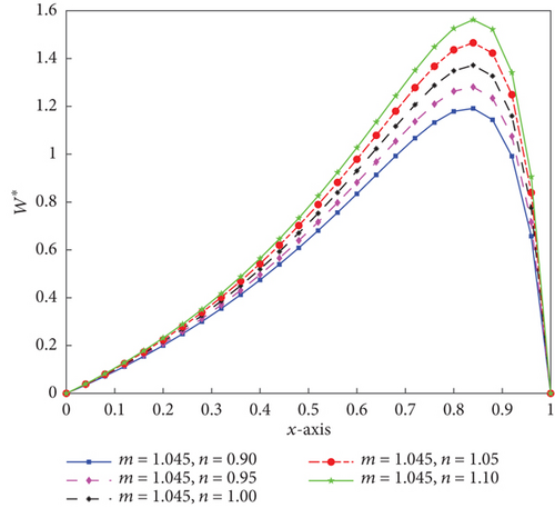
Figures 10, 11, and 12 illustrate the 1D transverse distribution of pressure performance caused by C₁ for non-Newtonian fluid flow for different values of the local power-law exponent (n) and consistency factor (M^⊛). For any constant value of n, M^⊛, and x^†, the LCCP is in ascending order of growing n value. Similar to what we see in the aforementioned graph, LCCP is rising as M^⊛ rises for the same value of n. This demonstrates that as the value of n increases for various values of M^⊛, the design of bearing will get better when taking both the effects of temperature and surface texture on LCCP. Additionally, a crucial component is the consistency factor.

For the fluid gap parameter w = 0.4, the LCCP and drag frictional force of transversal roughness are displayed in Table 6. It is obvious that the LCCP between b and c drops by about 8.9% for all values of n and M^⊛ = 0.530. In the same fashion, for all given values of n and M^⊛ = 0.530, the drag frictional force between c and b conditions almost goes to zero. The named table also indicates that the LCCP and drag force increase in each case as n and M^⊛ increase in value.

Table 6. Transversal texture W^⊛ and F^⊛ at different values of n and M^⊛.

Condition	M^⊛	W^⊛	n
Condition	M^⊛	F^⊛	0.9	0.95	1.0	1.05	1.1
a	0.53	W^⊛	0.3076	0.3272	0.3470	0.3672	0.3876
	0.53	F^⊛	1.5501	1.5502	1.5503	1.5502	1.5500
	1.0	W^⊛	0.5762	0.6130	0.6502	0.6880	0.7264
	1.0	F^⊛	1.5813	1.5816	1.5812	1.5806	1.5793
	1.045	W^⊛	0.6018	0.6401	0.6789	0.7184	0.7586
	1.045	F^⊛	1.5850	1.5852	1.5848	1.5840	1.5825

b	0.53	W^⊛	0.2820	0.2999	0.3179	0.3362	0.3549
	0.53	F^⊛	1.5502	1.5505	1.5506	1.5507	1.5507
	1.0	W^⊛	0.5284	0.5618	0.5956	0.6299	0.6649
	1.0	F^⊛	1.5817	1.5821	1.5822	1.5819	1.5816
	1.045	W^⊛	0.5518	0.5866	0.6890	0.6578	0.6941
	1.045	F^⊛	1.5853	1.5858	1.5974	1.5855	1.5846

c	0.53	W^⊛	0.3098	0.3295	0.3495	0.3698	0.3905
	0.53	F^⊛	1.5514	1.5517	1.5519	1.5520	1.5520
	1.0	W^⊛	0.5846	0.6217	0.6594	0.6977	0.7367
	1.0	F^⊛	1.5906	1.5915	1.5922	1.5926	1.5926
	1.045	W^⊛	0.6109	0.6496	0.6890	0.7291	0.7699
	1.045	F^⊛	1.5956	1.5966	1.5974	1.5978	1.5978

The values of the LCCP for each fixed n and M^⊛ are in the sequence of pressure due to condition (b)< condition (a)< condition (c) for all parameters, indicating that the LCCP is in the same order as the corresponding condition of pressure for non-Newtonian power-law fluid. For all values of n and M^⊛ throughout the entire fluid gap, condition (a)< condition (b)< condition (c) are in that order for frictional force. Additionally, for n = 0.90 and M^⊛ = 0.530, the load-bearing capacity for non-Newtonian between b and c differs by 0.7%, and the change in friction force for w = 0.4 is reduced by 2%.

This could be as consequence of the transverse roughness pattern, which obstructs the non-Newtonian fluid flow lubricant and increases pressure.

The LCCP and drag force of transversal roughness are illustrated in Table 7 for various n and M^⊛ effects corresponding to the aforementioned conditions and fluid flow gap. The sold body of slider bearing boundary temperatures is lower than or equal to the inflow intake temperature. When Cases i and ii for w = 0.4 have different sold body temperatures of bearing, the performance of the load changes by 6%. In terms of load and drag force, Case i performs a little bit better than Case ii for w = 1. When it comes to friction force, Cases i and ii just slightly differ from one another.

Table 7. Transversal texture W^⊛ and F^⊛ for different cases and values of n and M^⊛.

Case	n/M	W^⊛	w
Case	n/M	F^⊛	0.4	0.5	0.6	0.7	0.8	0.9	1.0
i	0.95/0.53	W^⊛	0.3380	0.2357	0.1617	0.1061	0.0632	0.0296	0.0030
	0.95/0.53	F^⊛	1.5508	1.3957	1.2787	1.1867	1.1123	1.0508	0.9989
	1.05/1.045	W^⊛	0.7427	0.5117	0.3461	0.2222	0.1274	0.0537	0.0041
	1.05/1.045	F^⊛	1.5857	1.4011	1.2684	1.1701	1.0956	1.0384	0.9937

ii	0.95/0.53	W^⊛	0.3167	0.2155	0.1428	0.0886	0.0471	0.0149	0.0103
	0.95/0.53	F^⊛	1.5502	1.3957	1.2792	1.1877	1.1136	1.0523	1.0007
	1.05/1.045	W^⊛	0.6947	0.4664	0.3039	0.1834	0.0919	0.0215	0.0332
	1.05/1.045	F^⊛	1.5835	1.4016	1.2711	1.1747	1.1017	1.0455	1.0017

iii	0.95/0.53	W^⊛	0.3245	0.2231	0.1502	0.0958	0.0541	0.0217	0.0037
	0.95/0.53	F^⊛	1.5506	1.3959	1.2793	1.1876	1.1134	1.0520	1.0002
	1.05/1.045	W^⊛	0.7123	0.4836	0.3206	0.1997	0.1078	0.0369	0.0183
	1.05/1.045	F^⊛	1.5854	1.4027	1.2716	1.1744	1.1007	1.0439	0.9995

iv	0.95/0.53	W^⊛	0.3384	0.2363	0.1626	0.1073	0.0647	0.0314	0.0051
	0.95/0.53	F^⊛	1.5514	1.3963	1.2792	1.1872	1.1128	1.0511	0.9992
	1.05/1.045	W^⊛	0.7437	0.5133	0.3484	0.2253	0.1311	0.0580	0.0007
	1.05/1.045	F^⊛	1.5886	1.4039	1.2710	1.1724	1.0976	1.0400	0.9949

The named table indicates that for any fluid gap, Case iv’s friction force and LCCP are lower than Case iii’s if the inflow inlet boundary temperature is lower than that of the solid body of the bearing. The temperature may increase across all the bearings if the pad temperature exceeds the slider temperature, which would decrease the bearing’s capacity to withstand loads and frictional force. In each case, we observe that LCCP and frictional force rise as the non-Newtonian parameters n and M^⊛ grow. In contrast, as the fluid gap rises, the LCCP and frictional values decrease.

For various inclination parameters of a power-law non-Newtonian fluid-type lubricant, Table 8 displays the LCCP and drag force of transversal roughness corresponding to the aforementioned conditions. The values of the LCCP and drag force for each fixed n and M^⊛ are in the order of pressure due to condition (b)< condition (a)< condition (c), indicating that the LCCP is in the same order as the relating condition of pressure. This table shows that the bearing performance increases under each condition as the values of n and M^⊛ increase and decreases under each condition when fluid film gap decreases.

Table 8. Transversal texture W^⊛ and F^⊛ for different values of n and M^⊛ versus inclination.

M^⊛	n	C_i	W^⊛			w
0.53			F^⊛	0.4	0.5	0.6	0.7	0.8	0.9	1.0
	0.95	a	W^⊛	0.3252	0.2253	0.1519	0.0968	0.0545	0.0215	0.0045
			F^⊛	1.5502	1.3955	1.2787	1.1870	1.1128	1.0514	0.9997
		b	W^⊛	0.2999	0.2098	0.1429	0.0917	0.0518	0.0203	0.0045
			F^⊛	1.5505	1.3957	1.2789	1.1872	1.1130	1.0515	0.9997
		c	W^⊛	0.3295	0.2281	0.1553	0.1006	0.0587	0.0259	0.0000
			F^⊛	1.5517	1.3968	1.2799	1.1880	1.1135	1.0519	1.0000
	1.05	a	W^⊛	0.3672	0.2513	0.1686	0.1070	0.0600	0.0236	0.0050
			F^⊛	1.5502	1.3950	1.2781	1.1864	1.1123	1.0511	0.9997
		b	W^⊛	0.3362	0.2339	0.1585	0.1013	0.0570	0.0223	0.0050
			F^⊛	1.5507	1.3953	1.2784	1.1866	1.1125	1.0512	0.9997
		c	W^⊛	0.3698	0.2545	0.1724	0.1114	0.0647	0.0285	0.0000
			F^⊛	1.5520	1.3966	1.2794	1.1875	1.1132	1.0517	1.0000

1.0	0.95	a	W^⊛	0.6130	0.4198	0.2804	0.1757	0.0954	0.0328	0.0163
			F^⊛	1.5816	1.4029	1.2734	1.1764	1.1021	1.0440	0.9980
		b	W^⊛	0.5618	0.3907	0.2633	0.1659	0.0900	0.0304	0.0166
			F^⊛	1.5821	1.4034	1.2740	1.1770	1.1025	1.0442	0.9979
		c	W^⊛	0.6217	0.4305	0.2929	0.1899	0.1107	0.0488	0.0000
			F^⊛	1.5915	1.4120	1.2813	1.1829	1.1070	1.0475	1.0000
	1.05	a	W^⊛	0.6880	0.4682	0.3111	0.1942	0.1049	0.0358	0.0181
			F^⊛	1.5806	1.4004	1.2705	1.1738	1.1000	1.0428	0.9978
		b	W^⊛	0.6299	0.4354	0.2920	0.1831	0.0990	0.0332	0.0185
			F^⊛	1.5819	1.4013	1.2713	1.1745	1.1005	1.0431	0.9977
		c	W^⊛	0.6977	0.4802	0.3254	0.2101	0.1221	0.0537	0.0000
			F^⊛	1.5926	1.4112	1.2797	1.1812	1.1057	1.0467	1.0000

1.045	0.95	a	W^⊛	0.6401	0.4382	0.2924	0.1829	0.0989	0.0335	0.0179
			F^⊛	1.5852	1.4035	1.2725	1.1748	1.1005	1.0429	0.9977
		b	W^⊛	0.5866	0.4077	0.2745	0.1726	0.0933	0.0310	0.0182
			F^⊛	1.5858	1.4041	1.2731	1.1754	1.1010	1.0431	0.9976
		c	W^⊛	0.6496	0.4498	0.3061	0.1984	0.1156	0.0510	0.0000
			F^⊛	1.5966	1.4139	1.2815	1.1822	1.1062	1.0469	1.0000
	1.05	a	W^⊛	0.7184	0.4886	0.3244	0.2021	0.1087	0.0365	0.0198
			F^⊛	1.5840	1.4008	1.2693	1.1719	1.0983	1.0416	0.9975
		b	W^⊛	0.6578	0.4544	0.3044	0.1905	0.1025	0.0338	0.0202
			F^⊛	1.5855	1.4017	1.2701	1.1726	1.0988	1.0419	0.9974
		c	W^⊛	0.7291	0.5018	0.3400	0.2196	0.1276	0.0561	0.0000
			F^⊛	1.5978	1.4130	1.2797	1.1804	1.1047	1.0461	1.0000

Even though it is slight, fluid film expansion as the temperature of the fluid lubricant rises for various values of n and M^⊛ results in the generation of LCCP in conditions a and b relative to c at w = 1.

6. Conclusions

The non-Newtonian lubricant fluid type layers in slider bearings, along with the surface texture and temperature effect, were demonstrated in this article using FEM. We looked at bearing performance measurements such as LCCP and drag force for 1D longitudinal and transverse surface texture types. The modified non-Newtonian power-law fluid type lubricant film equation was derived for the non-Newtonian fluid flow lubrication films of the bearing by using the local film thickness. The conclusions are succinctly summarized as follows:

•
The bearing performance (LCCP and drag force) for both types of nonparallel plane slider bearings improves. However, the LCCP and drag force are minimal when w = 1 (in parallel). In both model types, the opposite is true for drag force.
•
When power-law non-Newtonian fluid type is combined with the assumption that the slider’s temperature is higher than the pad’s, LCCP is higher for nonparallel bearing while it decreases to zero for parallel bearing (w = 1).
•
Under all of the aforementioned circumstances, as the non-Newtonian power-law constant parameters n and M^⊛ increase, so do the LCCP and drag force. The significance of taking into account the effects of the non-Newtonian power-law parameters n, M^⊛, and surface roughness is brought out by this.
•
1D longitudinal roughness slider bearings often have a lower pressure distribution than 1D transversal models.
•
This method’s drawback is that it is challenging to discretize the given irregular domain using a bilinear rectangular element, particularly in slider bearings with irregular upper and lower bounds.

Symbols

1D: one dimensional
δ: random distribution of roughness
μ: viscosity of the lubricant
μ_av: average viscosity across the film
ρ: density of the lubricant
ρ_av: average density across the film
σ²: variation of roughness
B: bearing width
p_r: Prandtl number
T: lubricant temperature
T_av: average temperature across the film
U: velocity of the moving surface
E: expected value operator
E_c: Eckert number
h: nominal film thickness
h₀: nominal film thickness at outlet
h_i: nominal film thickness at inlet
H_t: height of rough surface
k: thermal conductivity of lubricant
P: lubricant pressure
p_e: Peclet number
p_i: inlet pressure
v: velocity in the direction of the y-coordinate
w: h₀/h_i
W^⊛: load-carrying capacity of the bearing
x^†, y^†: transformed coordinate system
^⊛: a superscript “⊛” indicates the nondimensional quantity

Conflicts of Interest

The authors declare no conflicts of interest.

Funding

The authors declare that no funds, grants, or other support was received during the preparation of this manuscript.

Open Research

Data Availability Statement

The authors have nothing to report.

References

1 Yang Q., Huang P., and Fang Y., A novel Reynolds equation of non-Newtonian fluid for lubrication simulation, Tribology International. (2016) 94, 458–463, https://doi.org/10.1016/j.triboint.2015.10.011, 2-s2.0-84946118405.
10.1016/j.triboint.2015.10.011
Google Scholar
2 Lin J.-R., Non-Newtonian effects on the dynamic characteristics of onedimensional slider bearings: Rabinowitsch fluid model, Tribology Letters. (2001) 10, no. 4, 237–243, https://doi.org/10.1023/A:1016678208150, 2-s2.0-0038190382.
10.1023/A:1016678208150
CAS Web of Science® Google Scholar
3 Yadav S. K. and Sharama S. C., Performance comparison of partial and full textured thrust bearing operating with non-Newtonian lubricant, Applied Mechanics and Materials. (2014) 592, 1376–1380, https://doi.org/10.4028/www.scientific.net/AMM.592-594.1376, 2-s2.0-84905024383.
10.4028/www.scientific.net/AMM.592-594.1376
Google Scholar
4 Rao P. S. and Agarwal S., Effect of slip/no-slip on finite slider bearing using nonnewtonian micropolar fluid, Jurnal Tribologi. (2018) 19, 79–87.
Google Scholar
5 Chu L.-M., Hsu H.-C., and Chen J.-L., An analytical approach for analysis of slider bearings with non-Newtonian lubricants, Advances in Mechanical Engineering. (2014) 6, 404759, https://doi.org/10.1155/2014/404759, 2-s2.0-84893645946.
10.1155/2014/404759
Google Scholar
6 Nagaraju T., Sharma S. C., and Jain S., Performance of externally pressurized nonrecessed roughened journal bearing system operating with non-Newtonian lubricant, Tribology Transactions. (2003) 46, no. 3, 404–413, https://doi.org/10.1080/10402000308982644, 2-s2.0-0141750623.
10.1080/10402000308982644
CAS Web of Science® Google Scholar
7 Hsu Y. and Saibel E., Slider bearing performance with a non-Newtonian lubricant, Asle Transactions. (1965) 8, no. 2, 191–194, https://doi.org/10.1080/05698196508972093, 2-s2.0-0041964077.
10.1080/05698196508972093
Google Scholar
8 Oladeinde M., Edokpia R., and Unuigbe A., A study of static performance of fixed inclined slider bearings–a power law model, Journal of Applied Sciences and Environmental Management. (2011) 15, no. 4, 571–574.
Google Scholar
9 Walters K., Bates T., Coy R., and Williamson B., On the importance of nonnewtonian effects in journal bearing lubrication: a numerical approach, SAE Transactions. (1997) 106, 1065–1071.
Google Scholar
10 Haosheng C. and Darong C., Modified reynolds equation for non-Newtonian fluid with rheological model in frequency domain, Journal of Tribology. (2005) 127, no. 4, 893–898, https://doi.org/10.1115/1.2033005, 2-s2.0-27544438720.
10.1115/1.2033005
Google Scholar
11 Lin J.-R., Surface roughness effect on the dynamic stiffness and damping characteristics of compensated hydrostatic thrust bearings, International Journal of Machine Tools and Manufacture. (2000) 40, no. 11, 1671–1689, https://doi.org/10.1016/S0890-6955(00)00012-2, 2-s2.0-0033683854.
10.1016/S0890-6955(00)00012-2
Web of Science® Google Scholar
12 Guha S., Analysis of steady-state characteristics of misaligned hydrodynamic journal bearings with isotropic roughness effect, Tribology International. (2000) 33, no. 1, 1–12, https://doi.org/10.1016/S0301-679X(00)00005-0, 2-s2.0-0033626221.
10.1016/S0301-679X(00)00005-0
Web of Science® Google Scholar
13 Christensen H. and Tonder K., The hydrodynamic lubrication of rough bearing surfaces of finite width, Journal of Lubrication Technology. (1971) 93, no. 3, 324–329, https://doi.org/10.1115/1.3451579, 2-s2.0-85011886446.
10.1115/1.3451579
Google Scholar
14 Kumar B. R., A segregated supg/fem for thdl analysis in high speed slider bearings with injection effect, Journal of Tribology. (2001) 123, no. 4, 732–741, https://doi.org/10.1115/1.1339980, 2-s2.0-0035470787.
10.1115/1.1339980
Web of Science® Google Scholar
15 Rathish Kumar B. and Srinivasa Rao P., Streamline upwind Pertov-Galerkin finite element analysis of thermal effects on load carrying capacity in slider bearings, Numerical Heat Transfer Part A-Applications. (2000) 38, no. 3, 305–328, https://doi.org/10.1080/10407780050136549, 2-s2.0-1842811082.
10.1080/10407780050136549
Web of Science® Google Scholar
16 Sinha P. and Adamu G., THD analysis for slider bearing with roughness: special reference to load generation in parallel sliders, Acta Mechanica. (2009) 207, no. 1-2, 11–27, https://doi.org/10.1007/s00707-008-0094-7, 2-s2.0-68849098582.
10.1007/s00707-008-0094-7
Web of Science® Google Scholar
17 Adamu G. and Sinha P., Thermal and roughness effects in a tilted pad slider bearing considering heat conduction through the pad and slider, Proceedings of the National Academy of Sciences, India Section A: Physical Sciences. (2012) 82, no. 4, 323–333, https://doi.org/10.1007/s40010-012-0046-4.
10.1007/s40010-012-0046-4
Web of Science® Google Scholar
18 Desu Tessema G., Adamu Derese G., and Andargie Tiruneh A., Thermal and surface roughness effects on performance analysis of slider bearing via Petrov–Galerkin finite element method, Mathematical Problems in Engineering. (2022) 2022, no. 1, https://doi.org/10.1155/2022/4216136, 4216136.
10.1155/2022/4216136
Web of Science® Google Scholar
19 Tessema G. D., Derese G. A., and Tiruneh A. A., Analysis of thermal and surface roughness effects of slider bearing in the case of turbulent lubricant flow using finite element method, Research in Mathematics. (2023) 10, no. 1, article 2250492, https://doi.org/10.1080/27684830.2023.2250492.
10.1080/27684830.2023.2250492
Google Scholar
20 Tessema G. D., Derese G. A., and Tiruneh A. A., Performance analysis of thermal and surface roughness effect of slider bearings with unsteady fluid film lubricant using finite element method, Journal of Applied Mathematics. (2024) 2024, no. 1, https://doi.org/10.1155/2024/9993489, 9993489.
10.1155/2024/9993489
Google Scholar
21 Naduvinamani N. and Angadi A., Static and dynamic characteristics of rough porous Rayleigh step bearing lubricated with couple stress fluid, Lubricants. (2022) 10, no. 10, https://doi.org/10.3390/lubricants10100257.
10.3390/lubricants10100257
Web of Science® Google Scholar
22 Nb N. and Angadi A., On the dynamic characteristics of rough porous inclined slider bearing lubricated with micropolar fluid, Tribology Online. (2022) 17, no. 1, 59–70, https://doi.org/10.2474/trol.17.59.
10.2474/trol.17.59
Google Scholar
23 Gu Y., Cheng J., Xie C., Li L., and Zheng C., Theoretical and numerical investigations on static characteristics of aerostatic porous journal bearings, Machines. (2022) 10, no. 3, https://doi.org/10.3390/machines10030171.
10.3390/machines10030171
Web of Science® Google Scholar
24 Fang C., Zhu A., Zhou W., Peng Y., and Meng X., On the stiffness and damping characteristics of line contacts under transient elastohydrodynamic lubrication, Lubricants. (2022) 10, no. 4, https://doi.org/10.3390/lubricants10040073.
10.3390/lubricants10040073
Web of Science® Google Scholar
25 Jamshed W., Alanazi A. K., Isa S. S. P. M., Banerjee R., Eid M. R., Nisar K. S., Alshahrei H., and Goodarzi M., Thermal efficiency enhancement of solar aircraft by utilizing unsteady hybrid nanofluid: a single-phase optimized entropy analysis, Sustainable Energy Technologies and Assessments. (2022) 52, article 101898, https://doi.org/10.1016/j.seta.2021.101898.
10.1016/j.seta.2021.101898
Web of Science® Google Scholar
26 Raees M., Hussain M., Bibi N., Shigidi I. M., Pashameah R. A., Alzahrani E., El-Shorbagy M., and Safaei M. R., Energy transport analysis of the magnetized forced flow of power-law nanofluid over a horizontal wall, Journal of Magnetism and Magnetic Materials. (2022) 560, article 169681, https://doi.org/10.1016/j.jmmm.2022.169681.
10.1016/j.jmmm.2022.169681
Google Scholar
27 Dien I. and Elrod H., A generalized steady-state Reynolds equation for nonnewtonian fluids, with application to journal bearings, Journal of Lubrication Technology. (1983) 105, no. 3, 385–390, https://doi.org/10.1115/1.3254619, 2-s2.0-84962916070.
10.1115/1.3254619
Web of Science® Google Scholar
28 Ghosh M. K., Majumdar B. C., and Tech M. S. B., Fundamentals of fluid film lubrication, 2014, McGraw-Hill Education.
Google Scholar
29 Christensen H., Stochastic models for hydrodynamic lubrication of rough surfaces, Proceedings of the Institution of Mechanical Engineers. (1969) 184, no. 1, 1013–1026, https://doi.org/10.1243/PIME_PROC_1969_184_074_02.
10.1243/PIME_PROC_1969_184_074_02
Google Scholar
30 Zhu S., Sun J., Li B., Zhao X., Wang H., Teng Q., Ren Y., and Zhu G., Stochastic models for turbulent lubrication of bearing with rough surfaces, Tribology International. (2019) 136, 224–233, https://doi.org/10.1016/j.triboint.2019.03.063, 2-s2.0-85063759438.
10.1016/j.triboint.2019.03.063
Google Scholar
31 Schumack M., Application of the pseudospectral method to thermohydrodynamic lubrication, International Journal for Numerical Methods in Fluids. (1996) 23, no. 11, 1145–1161, https://doi.org/10.1002/(SICI)1097-0363(19961215)23:11%3C1145::AID-FLD459%3E3.0.CO;2-V.
10.1002/(SICI)1097-0363(19961215)23:11<1145::AID-FLD459>3.0.CO;2-V
CAS Web of Science® Google Scholar
32 Gururajan K. and Prakash J., Surface roughness effects in infinitely long porous journal bearings, Journal of Tribology. (1999) 121, no. 1, 139–147, https://doi.org/10.1115/1.2833795, 2-s2.0-0033041186.
10.1115/1.2833795
Web of Science® Google Scholar
33 Zienkiewicz O., Temperature distribution within lubricating films between parallel bearing surfaces and its effect on the pressures developed, Proc. Conference on Lubrication and Wear. (1957) 135.
Google Scholar
34 Pinkus O. and Sternlicht B., Theory of hydrodynamic lubrification, 1961, McGraw-Hill.
Google Scholar

Citing Literature

All articles

Bearing Performance Analysis of the Thermal and Surface Roughness Effects by Finite Element Method on Slider Bearings Through Non-Newtonian Fluid-Type Lubricant

Abstract

1. Introduction