Multiframe Target Localization With Strapdown Seeker Based on Self-Adaptive L-SHADE
Abstract
Strapdown seekers are increasingly used in the terminal guidance for the advantages of small size and low cost. However, due to the coupling of the seeker with the missile and its limited field of view, there is a risk of losing the target. This paper proposes a multiframe fusion target localization method for missiles with strapdown seekers, which can still obtain the target location through the recorded state data even when the target is lost. First, some preprocessing approaches are applied to ensure the accuracy of target location estimation with the linear success history–based adaptive differential evolution (L-SHADE) algorithm. Second, L-SHADE is extended into the self-adaptive linear success history–based adaptive differential evolution (SL-SHADE) algorithm to speed up the calculation of the target location to be applied onboard for actual flight use. Third, the simulation verifies its efficiency and further investigates the effect of parameter settings on the algorithm performance.
1. Introduction
The development of future wars puts forward the demand for the miniaturization of munitions. Therefore, strapdown seekers have been increasingly applied to the terminal guidance of missiles due to their small size, low cost, and high reliability. Compared with traditional platform seekers, strapdown ones cancel the mechanical parts and directly attach to the head of the missiles. The detection optical axis changes with the missile’s movement, but it also brings some problems. First, its instantaneous field of view (FOV) is small, so many guidance laws have been proposed considering FOV constraints [1–5]. The second is that the strapdown seekers cannot measure the line-of-sight (LOS) angular rate directly, and the typical approach is to estimate it through various filtering methods [6–10].
It is obvious that the precision strike of a munition is extremely dependent on the information provided by the seeker. However, the strapdown seeker has a limited FOV and is coupled with the missile’s movement. When the missile makes a large maneuver, or the target moves too fast, the seeker may lose the target. Also, the seeker may malfunction in operation. Given these situations, this paper proposes a new target localization method. The basic idea is to transform the localization problem into a single-objective nonlinear optimization problem. The target coordinate is generated. Combined with the state information of the missile, the LOS angular rate can be indirectly derived and thus input into the guidance law to calculate the guidance command.
As for solving nonlinear optimization problems, the methods mainly include gradient-based methods [11, 12], sequential quadratic programming [13], and metaheuristics [14, 15]. Among them, metaheuristic algorithms are well suited for complex and high-dimensional optimization problems. Moreover, they are generally more robust to noise in the objective function. In the real-world scenario, the state data measured by the missile is often biased, so here, we choose one of the metaheuristic algorithms, the differential evolution (DE) algorithm to solve the problem.
DE algorithm is a simple, yet effective tool for heuristic optimization proposed by Storn and Price [16–18]. It can be coded in a dozen lines and easily understood by general readers. Since then, DE families of methods have sprinkled into hundreds of variants [19–23]. Success history–based adaptive differential evolution (SHADE) is one of the representative DE algorithms featuring a different parameter adaptation mechanism [24, 25]. It was proposed by Tanabe and Fukunaga in 2013 as an improved version of adaptive differential evolution with optional external archive (JADE) [26]. They later developed L-SHADE by introducing a linear population size reduction (LPSR) mechanism [27]. It exhibited the best competitive performance among nonhybrid algorithms at the Congress on Evolutionary Computation (CEC) 2014 competition on real-parameter single-objective optimization.
As is well known, evolutionary algorithms are susceptible to control parameters. A standard DE has three main control parameters: the population size Np, scaling factor F, and crossover rate CR. According to the “no free lunch” (NFL) theorems [28], there is no universal solution applicable to all optimization problems. Thus, researchers have studied many adaptive mechanisms for adjusting the control parameters. Among them, the DE mutations operation can be classified into 30 novel schemes and six novel concepts [29]. In addition, population diversity is another key indicator guiding evolution in the right direction. The modification of initialization has also caught the attention of researchers. Common initialization strategies include random uniform distribution, Gaussian distribution, and Cauchy distribution.
Although the DE algorithm and its variants have been widely applied in many fields, there are also some shortcomings: (1) It is prone to premature convergence and falling into local optimality, and (2) the traditional DE algorithm has a strong dependence on parameter settings. To address these issues, improvements need to be made according to specific needs.
- 1.
The localization problem is transformed into a single-objective optimization problem. The objective function is set as the square of the error angle between the estimated and true LOS vectors.
- 2.
A new SL-SHADE algorithm is proposed which implements adaptive population initialization and nonlinear population size reduction (NLPSR). These operations can accelerate the convergence speed while ensuring the correctness of the results.
- 3.
The proposed algorithm is compared with L-SHADE, DE, and particle swarm optimization (PSO) in the 3D target localization problem, and the results confirm its effectiveness. Furthermore, the effects of error tolerance and frame size on the algorithm are analyzed.
The remainder of this paper is organized as follows. Section 2 introduces the coordinate systems and the LOS angle decoupling algorithm, then establishes the problem for optimization. Section 3 presents the overall architecture of the proposed target localization algorithm, including data preprocessing approaches and the SL-SHADE algorithm. Numerical simulations are presented in Section 4. The conclusion is given in Section 5.
2. Problem Formulation
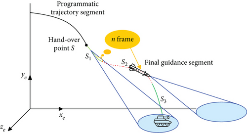
Figure 1 shows the application scenario. In the initial stage S1 of terminal guidance, the strapdown seeker can successfully recognize the target, and the guidance system works normally, during which the observed n frames of data are updated in real time and stored on the missile. When entering the stage S2, the target is beyond the seeker’s FOV due to the curved trajectory. To ensure the homing phase, the data stored in the stage S1, including the body line-of-sight (BLOS) angles measured by the seeker and the position and attitude information of the missile measured by the onboard combined navigation system, is used to solve for the target position in the Launch coordinate system. After that, combined with the current position of the missile, the LOS angle and angular rate can be calculated and input into the guidance system. In the stage S3, the seeker recaptures the target and continues the guidance until the interception ends. Through this method, the continuous, stable, and effective input of guidance information is satisfied during the whole process of terminal guidance, which ensures the steady progress of the homing phase.
2.1. Coordinate Systems and Conversion Relationships
In this section, a three-dimensional engagement geometry of a strapdown missile attacking a stationary or low-speed target is considered. To simplify, the impact of Earth’s rotation is neglected. The four relevant coordinate systems are defined in Figure 2, and the detailed description is given below.
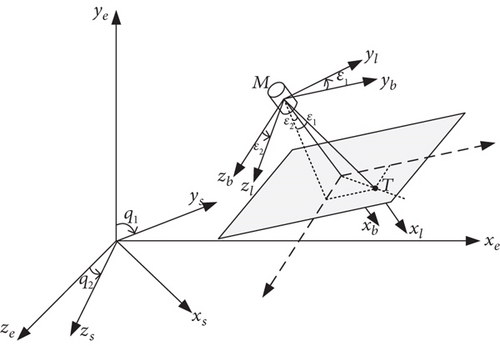
2.1.1. Body Coordinate System Ob − xbybzb
The origin Ob is selected at the mass center of the missile; Obxb coincides with the longitudinal axis of the missile and points forward; Obyb is within the main symmetry plane of the missile and perpendicular to Oxb, positive upwards; Obzb forms the right-handed rule with Obxb and Obyb.
2.1.2. Launch Coordinate System Oe − xeyeze
The origin Oe coincides with the launch point; Oexe points towards the direction of launch aiming within the horizontal plane of the launch point; Oeye is perpendicular to the horizontal plane of the emission point and points upwards; Oeze forms the right-handed rule with Oexe and Oeye.
2.1.3. LOS Coordinate System Os − xsyszs
The origin Os is selected at the mass center of the missile; Osxs points to the missile-to-target direction; Osys is upwards within the vertical plane and perpendicular to Osxs; Oszs forms the right-handed rule with Osxs and Osys.
2.1.4. BLOS Coordinate System Ol − xlylzl
The origin Ol is selected at the mass center of the missile; Olxl points to the missile-to-target direction; Olyl is upwards in the xbObyb plane; Olzl forms the right-handed rule with Olxl and Olyl.
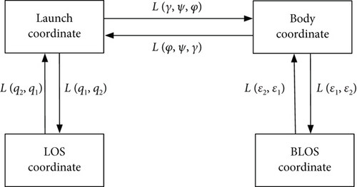
The conversion relationship of coordinate systems is shown in Figure 3, where φ, ψ, and γ denote the pitch, yaw, and roll angle, respectively; q1 and q2 denote the LOS vertical angle and azimuth angle; ε1 and ε2 denote the BLOS vertical angle and azimuth angle.
2.2. LOS Angle Decoupling Algorithm
Since the strapdown seeker is fixed on the missile rigidly, the seeker’s optical axis is aligned with the body axis Obxb. The BLOS angles ε1 and ε2 can be measured directly. However, the missile position [xm, ym, zm] is given under the launch system, while the attitude angles [φ, ψ, γ] are given in the launch system. To obtain LOS angles q1 and q2 in the inertial space used for the guidance law, it is necessary to eliminate the coupling between the strapdown seeker and the missile attitude motion. In this article, all quantities are unified into the LOS coordinate system for calculation.
2.3. Target Localization Problem for Optimization
When the target is located within the FOV range, data including [ε1, ε2, xm, ym, zm, φ, ψ, γ] is recorded and stored as n frames. Once an unexpected situation occurs, this data is called to calculate the target position. This section constructs the problem for optimization and defines the objective function.
3. Proposed Target Localization Algorithm
Figure 4 illustrates the proposed target localization algorithm for the vehicle with a strapdown seeker.
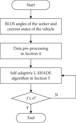
The proposed algorithm initially receives BLOS angles [ε1, ε2] of the strapdown seeker and the flight states including position [xm, ym, zm] and attitude angles [φ, ψ, γ] of the missile. Record n frames of data. Then, rigid preprocessing steps involving key frame selection and search range modification are implemented. In this case, the informative data is reserved, and the algorithm will not converge on the wrong solution. Later, the constructed data is utilized to optimize the target localization model with the proposed SL-SHADE algorithm. The algorithm helps to find the ideal solution in a constrained space without the gradient information. Finally, the target location [xt, yt, zt] in the launch coordinate system is derived. As missile data updates, repeat the above steps to obtain the latest target position.
3.1. Data Preprocessing Approaches
This section applies some rigid data preprocessing approaches to the input data. This works to avoid converging to the wrong solution.
3.1.1. Key Frame Selection
This method estimates the target position through geometric localization. For data selection, the sampling interval should not be too short, otherwise the observations will be highly overlapped, resulting in less data. Insufficient data deteriorates the performance of the algorithm. On the other hand, the number of frames n should also not be too many, otherwise it will increase the burden of the algorithm and prolong the computational time. Therefore, a suitable size of n must be chosen.
In general, it is acceptable to select the nearest n frames of data. However, a special case needs to be noted—the tangent line of the ballistic trajectory coincides with the LOS vector. As shown in Figure 5, if lateral maneuvers are not considered, it means that the flight path angle is equal to the LOS vertical angle, that is, q = ϑ. At this moment, any point on the LOS line can satisfy the angle constraint, rendering the measurement data meaningless.
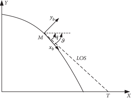
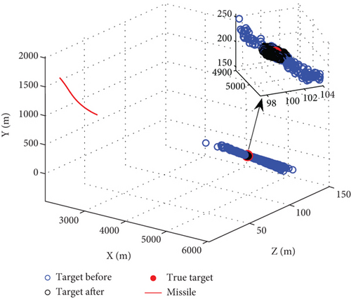
To avoid this, certain key frames must be included in the stored data. For example, the initial data can be bound to the missile before launch, and during the terminal guidance, the data at certain time intervals can be stored sequentially within the first k frames, while the most recent data is updated chronologically starting from the k + 1 frame. The comparison before and after key frame selection is shown in Figure 6. The red curve is the missile trajectory. The red dot is the true target position. The blue point is the original result, and the black one is the modified result. The algorithm results may converge to any point on the straight line before, while gathering near the true value after the improvement.
3.1.2. Search Range Modification
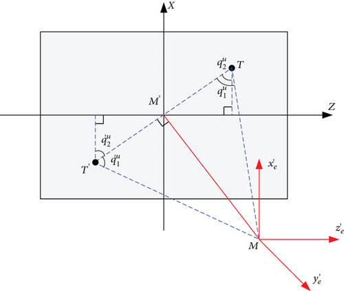
In the usual case, the parameter search range is fixed. In this problem, it can be set as the missile range. However, it poses the problem that when the missile range is large enough, two acceptable target points can be found that satisfy the angular constraints. As shown in Figure 7, translate the launch coordinate Oe − xeyeze to the mass center of the missile as , and targets T and T′ are symmetric about the missile’s projection point M′ on the horizontal plane. Because , according to (9), and ; that is, they are equivalent in terms of objective functions. However, in the light of the actual situation, T is the correct solution.
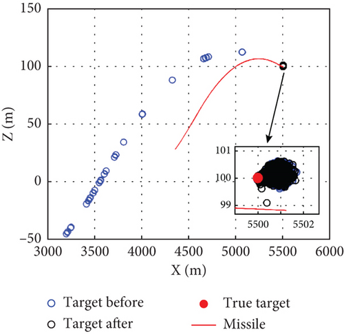
Consider striking a ground target as an example; the quantity to be sought is the 2D target coordinate under the launch system. The result is shown in Figure 8, where the red curve is the missile projected coordinate in the ground plane, the red dot is the true target position, the blue point is the original result, and the black point is the modified result. The algorithm before has a high probability of finding the error solution which is symmetric with the true value and changes constantly with the movement of the missile. However, after modification, this problem does not exist, with all the solutions converging to the neighborhood of the true value.
3.2. Self-Adaptive L-SHADE Algorithm
In this section, we first describe L-SHADE in Sections 3.2.1–3.2.6. Then, in Sections 3.2.7 and 3.2.8, we propose the SL-SHADE, which features the improving NLPSR and adaptive initialization strategy. Finally, the overall SL-SHADE algorithm is summarized in Section 3.2.9.
Like the classic DE algorithm, L-SHADE also consists of four basic operators: initialization, mutation, crossover, and selection. Parameter adaptation and LPSR are employed during the evolution process. The L-SHADE algorithm incorporates LPSR in the SHADE algorithm. Thus, the parameters CR and F are automatically adjusted based on a historical memory of successful parameter settings and the population size Np is continuously reduced following a linear function.
3.2.1. Initialization
3.2.2. Mutation
3.2.3. Crossover
3.2.4. Selection
3.2.5. Control Parameter Adaptation Based on Historical Memory
As shown in Table 1, L-SHADE maintains a historical memory with H entries for both CR and F as MCR and MF. The contents of MCR,k, MF,k(k = 1, ⋯, H) are all initialized to 0.5 in the beginning and then updated at the end of each generation based on Algorithm 1. k is initialized to 1 and incremented whenever a new element is inserted into the history. If k > H, k is set to 1.
| Index | 1 | 2 | ⋯ | H − 1 | H |
|---|---|---|---|---|---|
| MCR | MCR,1 | MCR,2 | ⋯ | MCR,H−1 | MCR,H |
| MF | MF,1 | MF,2 | ⋯ | MF,H−1 | MF,H |
In each generation, CRi and Fi values that succeed in selection are recorded as SCR and SF, and at the end of the generation, the memory contents MCR and MF are updated using Algorithm 1.
-
Algorithm 1: Memory update in L-SHADE algorithm.
-
Input: crossover vector ug, parent vector xg, success value SCR, SF, original memory contents
-
Output: updated memory contents
-
Main Loop:
-
1: if SCR ≠ ∅ and SF ≠ ∅ then
-
2: if or max(SCR) = 0 then
-
3:
-
4: else
-
5:
-
6: end if
-
7:
-
8: k + +
-
9: if k > H then
-
10: k = 1
-
11: end if
-
12: else
-
13:
-
14:
-
15: end if
Better controller parameter values tend to generate individuals that are more likely to survive. This method helps propagate better values to the following generations, improving the progress rate and avoiding premature convergence.
3.2.6. LPSR
3.2.7. Improving NLPSR
Figure 9 compares the changes in population size with evaluation iterations for different population reduction strategies. The proposed NLPSR strategy maintains a population reduction rate like that of LPSR at an early stage. This allows enough time for individuals to evolve, which helps to maintain population diversity and enhance the global search capability of the algorithm. In the middle and late stages, the population size is significantly reduced, which can improve algorithm efficiency, enhance local search capabilities, and prevent waste of computational resources. This improving strategy requires less simulation space, which can accelerate the speed and satisfy the demand for actual flight use.

3.2.8. History-Based Initialization
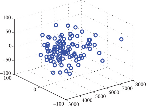
Due to the continuity of target movement, target positions over time are correlated. Therefore, we propose history-based initialization to utilize previous optimal solutions to guide the generation of new populations, thus achieving faster progress in the evolutionary search. When the target location found in this trial meets specific conditions (i.e., the fitness value f(·) or the iteration number g less than a set value), it is considered to be ideal. The result is saved as the history optimal vector and used to initialize population vectors of the next trial. As a result, in the initial stage of each simulation, there is a greater probability of finding a solution vector that satisfies the conditions than random initialization.
Figure 10 shows a comparison of two initialization methods in 3D space. Randomly initialized individuals are distributed evenly, while history-based ones are closely arranged and symmetrically distributed with . Based on the requirements of the scenario and the performance of historical search results, we can choose an appropriate initialization strategy between the two initialization methods.

3.2.9. Overall Implementation
Finally, the overall SL-SHADE algorithm is shown in Algorithm 2. Lines 2–7 implement the adaptive initialization operation combining random initialization with history-based initialization. Lines 10–18 and line 30 show Algorithm 1, updating CR and F based on historical memory. Line 32 shows the NLPSR strategy. The remaining part shows the loop of mutation, crossover, and selection.
-
Algorithm 2: The SL-SHADE algorithm.
-
Input: BLOS angles ε1, ε2, missile position xm, ym, zm, attitude angles φ, ψ, γ, population size Np, search upper and lower boundaries XH, XL, history optimal vector , maximum iteration gmax, termination value ε, memory size H, best rate p, archive rate, maximum and minimum population size
-
Output: target position xt, yt, zt, updated history optimal vector
-
Main Loop:
-
1:g = 1, Np = Npinit, Archive A = ∅
-
2:Adapt search boundaries according to (12)
-
3:if then
-
4: Initialize population
-
5:else
-
6: Initialize population randomly
-
7:end if
-
8:Set all values in MCR, MF to 0.5
-
9:while g < gmax or f > ε do
-
10: SCR = ∅, SF = ∅
-
11: for i = 1 to Np do
-
12: ri = Select from [1, H] randomly
-
13: if then
-
14:
-
15: else
-
16:
-
17: end if
-
18:
-
19: Generate trial vector according to current-to-pbest/1 with archive
-
20: end for
-
21: for i = 1 to Np do
-
22: if then
-
23: ;
-
24: else
-
25:
-
26: end if
-
27: if then
-
28: , ,
-
29: end if
-
30: Shrink A if necessary
-
31: Update MCR and MF (algorithm 1)
-
32: Apply NLPSR strategy
-
33: end for
-
34: g + +;
-
35:end while
-
36:if g < gmax/2
-
37:
-
38:end if
-
39:Return as the best-found solution
4. Numerical Simulations
In this section, experiments are conducted to validate the effectiveness of the proposed SL-SHADE algorithm. We first compare the SL-SHADE algorithm with L-SHADE [27], DE [17], and PSO [30] in estimating airborne targets and then investigate the performance of SL-SHADE under different input uncertainties, error tolerances, and frame numbers.
The PC configuration is as follows: Windows 11, CPU: Intel Core i9-13900H 2.60 GHz, RAM: 32 GB.
A 6–degrees of freedom (DOF) missile trajectory model is established, and the strapdown seeker model with the target localization algorithm is embedded into it. The missile is launched at ground (0, 0, 0) with initial lead angles φM(0) = 65°. The output frequency of the strapdown seeker is set as 50 Hz. Giving gyroscope drift of 1°/h and strapdown seeker’s tracking accuracy of ±2 pixels, the BLOS angles and attitude angles are set to obey normal distribution, with the BLOS angle error nb ~ N(0, 0.12)( °) and the attitude angle error nz ~ N(0, 0.052)( °). When the missile-to-target distance is less than 2 km, the position estimation algorithm is performed. The airborne stationary target is first set to [5000, 200, 100].
Table 2 shows the parameter settings of the four algorithms.
| Parameters | Settings |
|---|---|
| Maximum iteration gmax | 100D |
| Upper bound XH | (8000, 1000, 1000) |
| Lower bound XL | (3000, −100, −1000) |
| SL-SHADE | |
| Maximum population size | 18D |
| Minimum population size | 4 |
| Best rate p | 0.11 |
| Archive rate | 1.4 |
| Memory size H | 5 |
| DE | |
| Population size Np | 50 |
| Scaling factor F | 0.8 |
| Crossover rate CR | 0.9 |
| PSO | |
| Inertia weight w | 0.7 |
| Cognitive coefficient c1 | 1.5 |
| Social coefficient c2 | 1.5 |
4.1. Comparison Results
This subsection first compares the performance of the four algorithms under 40 frames of fixed data input and then investigates the performance of DE algorithms in a real-time data update environment.
The collected 40 frames of data were used as input to validate the offline performance of the algorithms. After 100 independent runs, the results including the mean, standard deviation (std), average value of the objective function, and success rate (SR) of the four algorithms are obtained as follows. When the difference between the estimated value of the target position and the true value is not more than 25 m, it is considered successful.
As shown in Table 3, the results of SL-SHADE, L-SHADE, and DE are all relatively accurate, with L-SHADE performing the best, SL-SHADE the second best, and DE the worst. This is because SL-SHADE sacrifices part of its accuracy in pursuit of speed, while the parameters of DE are fixed and cannot guide the direction of evolution based on the results. The SR of PSO is only 30%, which indicates that the classic version of PSO is not suitable for dealing with such kind of complex and noisy problems. It is also worth noting that due to measurement noise, the target position estimation will not be exactly equal to its true position [5000, 200, 100].
| Algorithm | xt (m) | yt (m) | zt (m) | fave | SR (%) |
|---|---|---|---|---|---|
| Mean (std) | Mean (std) | Mean (std) | |||
| SL-SHADE | 5001.42 (6.15e−5) | 200.28 (3.90e−5) | 100.01 (4.68e−6) | 3.8495e−11 | 100 |
| L-SHADE | 5001.42 (5.39e−5) | 200.28 (3.46e−5) | 100.01 (4.26e−6) | 3.8495e−11 | 100 |
| DE | 5001.42 (6.80e−5) | 200.28 (4.38e−5) | 100.01 (4.90e−6) | 3.8495e−11 | 100 |
| PSO | 5255.06 (452.49) | 18.67 (201.53) | 115.60 (27.86) | 1.1725e−04 | 30 |
Then, the target localization algorithm is embedded into the missile 6DOF model, and the input data is updated in real time to verify the online performance of the algorithms. Here are the results of SL-SHADE, L-SHADE, and DE. gave indicates the average number of iterations that satisfy f < 10−5.
As shown in Table 4, both SL-SHADE and L-SHADE algorithms can successfully estimate the target location. The results of SL-SHADE and L-SHADE are relatively similar with good performance, while the results of DE are less desirable with larger variance and lower SR. However, the average iteration gave of SL-SHADE is much smaller than that of L-SHADE and DE, indicating that the efficiency of the SL-SHADE algorithm has been greatly improved. On the current device, the average simulation time is 0.02 s. When applied on the missile, a high-frequency CPU can be utilized to meet the 0.1-s guidance cycle requirement. Therefore, the requirements for onboard use can be met.
| Algorithm | xt (m) | yt (m) | zt (m) | fave | gave | SR (%) |
|---|---|---|---|---|---|---|
| Mean (std) | Mean (std) | Mean (std) | ||||
| SL-SHADE | 5002.40 (3.80) | 198.11 (3.82) | 99.92 (0.98) | 5.2688e−6 | 37.70 | 100 |
| L-SHADE | 5002.40 (3.80) | 198.11 (3.82) | 99.92 (0.98) | 5.2688e−6 | 42.20 | 100 |
| DE | 5002.41 (3.84) | 198.08 (4.15) | 99.92 (0.98) | 5.2714e−6 | 52.11 | 99.96 |
4.2. Performance Under Different Input Uncertainties
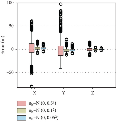
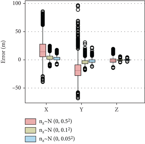
Input uncertainties of BLOS angles and attitude angles directly affect the estimation accuracy of the target position. To investigate the effect of input uncertainty on the results, the stds of BLOS angle error and attitude angle error are set to 0.5, 0.1, and 0.05, respectively, in this section. The input frame number n is uniformly set as 40.
The simulation results are shown in Figure 11 and Table 5. As shown in Figure 11, the deviation of the output target position gradually increases as the deviation of the measured angles increases, indicating that the estimation accuracy decreases. Among them, the scatter ranges of xt and yt are similar, while the scatter of zt is smaller, which means that the estimation result of zt is the most accurate.
| BLOS angle | Attitude angle | xt (m) | yt (m) | zt (m) |
|---|---|---|---|---|
| Std (°) | Std (°) | Mean (std) | Mean (std) | Mean (std) |
| 0.05 | 0.05 | 5002.27 (2.58) | 198.20 (2.42) | 99.93 (0.67) |
| 0.1 | 0.05 | 5002.40 (3.80) | 198.11 (3.82) | 99.92 (0.98) |
| 0.5 | 0.05 | 5003.05 (16.11) | 198.29 (18.82) | 99.84 (3.95) |
| 0.1 | 0.1 | 5004.11 (5.08) | 196.29 (4.87) | 99.82 (1.34) |
| 0.1 | 0.5 | 5017.48 (18.86) | 182.30 (17.41) | 99.04 (5.11) |
Comparing the results under different BLOS angle errors and different attitude angle errors, the attitude angle uncertainty has a greater impact on the results. As the deviation of the attitude angle increases, the deviation of the mean and median from the true value both increases, with the mean deviation of xt 17.48 m and the mean deviation of yt 17.7 m. The accuracy of the estimation greatly deteriorates. In the process of practical use, it is necessary to use the precise gyroscope to ensure the accuracy of attitude angle measurement. When the target is lost, to hit a 15 × 5 × 15 m target, it is necessary to ensure that the BLOS angle std and attitude angle std are both 0.05°.
4.3. Performance Under Different Error Tolerances
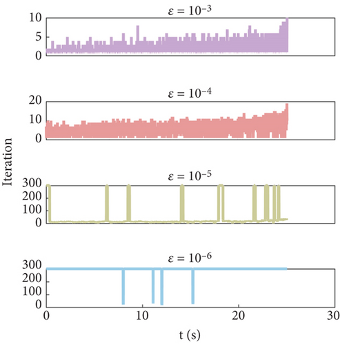
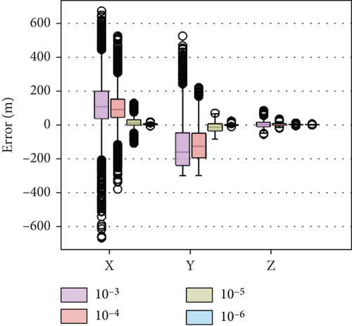
When used onboard, to reduce the computational pressure and speed up the estimation speed, a threshold condition can be added. When the objective function f < ε, the optimization process terminates, and the target location is directly output. The error tolerance ε is related to the angular error Δθ; for example, ε < 10−6 means Δθ < 10−3.5. In this section, ε is set as 10−3, 10−4, 10−5, and 10−6 respectively, to investigate the effect of error tolerances on the optimization performance.
The simulation results are shown in Figure 12 and Table 6. The iteration number decreases as the error tolerance increases, while the resultant error increases as the error tolerance increases. Figure 12(a) indicates that as the requirement for accuracy increases, more iterations are needed to meet the requirement. From Figure 12(b), it can be seen that when the error tolerance is set to 10−4, the maximum error of xt exceeds 400 m, indicating that such a large error tolerance will greatly reduce the accuracy of the result or even make the algorithm invalid. Comparing the results of xt, yt, zt, the accuracy of zt is much higher than that of xt and yt, which indicates that the algorithm is more sensitive to the lateral changes of the target coordinates. The estimated xt is high, and yt is low. Both xt and zt have outliers, while yt does not. This is due to the fact that in (9), xt and zt are positively proportional and therefore vary consistently. As the missile-to-target distance approaches, parameter range adaptation makes the lower bound continuously rise, and the estimation result accuracy also continuously improves, so xt and zt values tend to converge around the true value. However, yt is alone on the numerator and thus has been oscillating uniformly.
| Error tolerance ε | xt (m) | yt (m) | zt (m) | gave |
|---|---|---|---|---|
| Mean (std) | Mean (std) | Mean (std) | ||
| 10−3 | 5109.59 (170.82) | 73.67 (143.52) | 101.84 (21.20) | 1.89 |
| 10−4 | 5098.67 (110.44) | 83.63 (99.78) | 101.07 (7.56) | 6.17 |
| 10−5 | 5013.46 (31.42) | 185.25 (28.63) | 100.06 (2.00) | 37.70 |
| 10−6 | 5002.40 (3.81) | 198.11 (3.83) | 99.92 (0.98) | 298.81 |
As can be seen from Table 6, the std of xt is the largest, yt the second, and zt the smallest under the uniform error tolerance. As the error tolerance decreases, the coordinate std also decreases and eventually approaches zero.
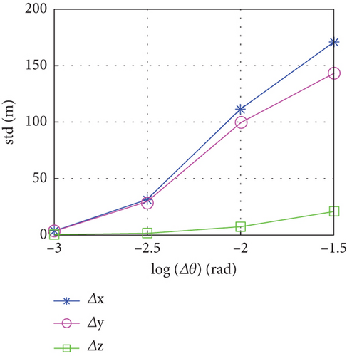
Since f is proportional to (Δθ)2, the relationship between the estimation error and the accuracy of Δθ is plotted in Figure 13. The trends of xt and yt are identical, with the curve declining rapidly at first and then slowing down, while zt declines smoothly and slowly. The stds of xt, yt, zt are 171, 144, and 21 m when the angle between the assumed and true LOS is 0.03 rad. As Δθ goes down to 0.001 rad, the stds of xt, yt, zt decrease to 3.81, 3.83, and 0.98 m. The error tolerance levels exhibit marginal effects.
4.4. Performance Under Different Frame Numbers
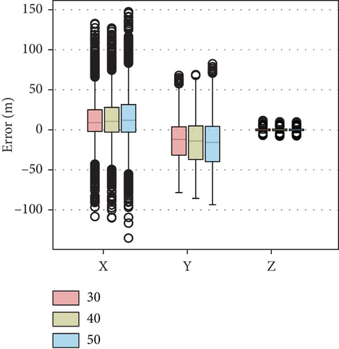
In the above simulation, the input frame number n was uniformly set as 40. In this section, n is set as 30, 40, and 50, respectively, to investigate the influence of different frame numbers on the optimization performance. The error tolerance is set as ε = 10−5.
The simulation results are shown in Figure 14 and Table 7. As can be seen, the number of input frames has a small effect on the iteration numbers. It is generally assumed that the more input frames, the greater the amount of data, and the more accurate the estimation results are. However, the simulation results show the opposite. This is because, after the key frame selection, the first k frames of data already have enough information. At this time, increasing the frame number will instead increase the proportion of the data with a short period in the total data, affecting the accuracy of the algorithm. Therefore, it is possible to use as few input frames as possible while ensuring normal operation.

| Frame number n | xt (m) | yt (m) | zt (m) | gave |
|---|---|---|---|---|
| Mean (std) | Mean (std) | Mean (std) | ||
| 30 | 5011.79 (29.24) | 187.23 (26.14) | 100.07 (1.99) | 21.15 |
| 40 | 5013.46 (31.42) | 185.25 (28.63) | 100.06 (2.00) | 20.94 |
| 50 | 5014.59 (34.13) | 183.71 (31.51) | 100.02 (1.88) | 20.87 |
5. Conclusion
To cope with the situation where the seeker loses the target, we design a new target localization algorithm for missiles with strapdown seekers. Multiframe data is used to find the target position based on the proposed SL-SHADE algorithm.
The performance of the localization algorithm is thoroughly investigated. The SL-SHADE algorithm is validated by simulation to outperform L-SHADE, DE, and PSO because it can locate 3D airborne targets with fewer iterations while ensuring accuracy. Under the error tolerance of 10−6, the result accuracy can reach within 13.91 m. The zt estimation accuracy is superior to xt and yt. The study also investigates the impact of error tolerance and frame number on the results, demonstrating that by adjusting the termination error condition in simulations, estimation accuracy and time can be balanced. Moreover, fewer input frames are preferable within the allowable range.
Conflicts of Interest
The authors declare no conflicts of interest.
Funding
This work was supported by the National Natural Science Foundation of China (U21B200527).
Open Research
Data Availability Statement
The data that supports the findings of this study are available on request from the corresponding author, upon reasonable request and with permission of laboratory confidentiality agency permission.


