Early Warning of Low-Frequency Oscillations in Power System Using Rough Set and Cloud Model
Abstract
The stability of the power system is largely affected by low-frequency oscillations, so early warning research on low-frequency oscillations in power grids has become an urgent task. Traditional low-frequency oscillation early warning methods are still deficient in handling incomplete and highly discrete information. Compared with the existing methods, we have pioneered a synergistic mechanism of discrete attribute screening and continuous probabilistic feature fusion by combining the dynamic attribute approximation algorithm of rough sets with the cloud model, which effectively solves the loss of information caused by the discretization of continuous data in the traditional methods. Firstly, we analyze the principle of grid oscillation, use rough sets to process the raw data and indicators, remove redundant attributes, and get the set reflecting the relationship of different attributes. Then we construct a standard cloud based on grid operation data and a comprehensive cloud based on PMU data and obtain the oscillation warning evaluation. Finally, through the validation and simulation of 10 machine and 39 node systems in New England, as well as the comparison with other methods, the rationality and effectiveness of the proposed method are proved to be of theoretical and practical application value.
1. Introduction
Low-frequency oscillations (LFOs) are significant concerns in power systems, affecting the stability and reliability. These oscillations typically occur in the frequency range from 0.1 to 2.0 Hz and can lead to inefficient power transmission, increased wear on equipment, and power system instability or blackouts. At present, there are a variety of specific methods for the LFO early warning of power grid at home and abroad, all of which can analyze LFO to a certain extent. They all have their advantages and disadvantages. The artificial neural network diagnosis method used in references [1–3] does not need to build a relevant knowledge base. However, for example, in reference [4], it is difficult to obtain a complete sample set for its training. Therefore, the diagnosis method of artificial neural network is only used in the diagnosis of small and medium-sized and simple power systems for the time being. There is also a Bayesian network diagnosis method used in references [5–7]. The principle of Bayesian network is simple, easy to understand, and insensitive to data loss. As can be seen in reference [8], the required training parameters are also few. To obtain the conditional probability distribution of each node in the network structure, it is difficult to determine actual problems and rely on the expert knowledge and relevant statistical analysis. The Prony algorithm mentioned in references [9, 10] adopts a linear combination of exponential terms to fit the equally spaced sampled data, from which information such as amplitude, phase, damping factor, and frequency of signals can be analyzed to objectively reflect the frequency characteristics. Although the model D-S evidence algorithm in references [11–13] can complete the LFO early warning task to a certain extent, its weight and conditional probability acquisition meet weaker conditions than the Bayesian probability theory, and it has the ability to directly express “uncertainty” and “don’t know.” However, as mentioned in reference [14], under the feature analysis of high dimension, contradictory evidence cannot be effectively processed, and with the growth of data, the amount of computation increases exponentially. In reference [15], when the reasoning chain is long, it is inconvenient and cumbersome to use evidence theory. Similarly, the hidden Markov algorithm in references [16, 17] has been applied to LFO and other power grid stability early warning due to its self-learning characteristics. But it has high requirements on input signals, requires a large amount of computation in learning, and has poor detection efficiency and real-time performance. If the long-sequence early warning task is carried out like that in reference [18], it can be used as an example. It is easy to produce error accumulation, making the accuracy difficult to meet the requirements.
- 1.
In view of the complex and incomplete operation data of the power system, rough sets are used to process real-time and historical data of the power grid.
- 2.
Innovative combination weights are constructed by combining attribute importance and knowledge granularity with expert methods to make the comprehensive evaluation of power grid warning more objective and precise.
- 3.
Historical data are used to construct a standard cloud, and the real-time PMU data are used to construct a comprehensive evaluation cloud to determine the early warning risk evaluation level through affiliation analysis.
In Section 2, this paper introduces the relevant fundamental theories. In Section 3, it constructs the early warning model of LFO in power grid based on the knowledge proposed in the previous section. In Section 4, it carries out the simulation and verification based on the New England 10-machine and 39-node example. Section 5 concludes this paper.
2. Fundamental Theory
2.1. Rough Set Principle
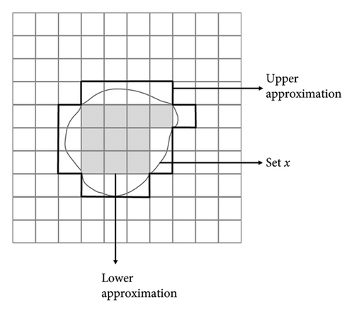
The rough set theory is a mathematical approach to dealing with vagueness and uncertainty by approximating sets with a pair of sets called the lower and upper approximations. In the definition and research of rough sets, feature reduction algorithms based on the attribution importance are all heuristic algorithms. That is, using heuristic information as the criterion to measure importance, adding non-nuclear conditional attributes with the greatest attribute importance to the kernel attribute set, or deleting conditional attributes with the least attribute importance one by one can meet the final condition. In the rough set theory, knowledge granularity represents the degree of fine division of knowledge (partition granularity), which can be used to measure the importance of equivalent categories related to knowledge, while attribute importance is to evaluate the importance of attribute kernel in a knowledge system and screen the most important attribute features. It can play a key role in attribute reduction of rough sets by classifying knowledge horizontally and analyzing it objectively by using the granularity function and then determining the weight vertically by combining with the attribute importance. Figure 1 shows a schematic diagram of rough set principle.
Please see the appendix for the formulas related to attribute importance-knowledge granularity, and here are the important formulas for the algorithms.
2.2. Cloud Model Theory
Cloud model theory solves the problem of uncertainty in transformations between qualitative and quantitative attributes by describing and calculating expectations (Ex), entropy (En), and hyperentropy (He). Comprehensive evaluation cloud: Due to the different relevance or independence between the sublayers corresponding to all levels of indicators in the power grid risk evaluation system, the algorithms used are not the same. Therefore, we use the integrated cloud algorithm and the standard operational algorithm for affiliation analysis to determine the risk level of the grid. The specific formulas are as follows.
3. Construction of Power Grid Early Warning Model Based on Rough Set and Cloud Model
3.1. Data Preprocessing
3.2. Rough Set Reduction Based on Grid Data
In the process of LFO warning, we use the approximation ability of rough sets to analyze and process the grid operation data and approximate the operation indexes according to the data to meet the current grid state.
-
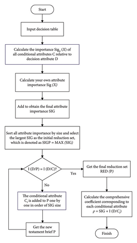
Step 1: Input a complete information system S = {U, R, V, F}, where U is the universe of discourse, and R = C ∪ D, C is the set of conditional attributes corresponding to the grid metrics, which is selected based on the characteristics of the power system; D is the decision attribute set, which generally is whether the fault or not, fault area, and power system operation state.
-
Step 2: Calculate the comprehensive attribute importance of each condition attribute in the condition attribute set and take the condition attribute set corresponding to the largest value as the initial set of heuristic information, denoted as SIGP, and SIGP = MAX(SIG).
-
Step 3: Compute the knowledge granularity I(D/C) of the set with the addition of the remaining conditional attributes in order according to the importance ranking of the comprehensive attributes.
-
Step 4: Determine whether the information amount (granularity entropy) of the reduction set is equal to the original reduction set. If not, continue to add the remaining condition attributes and calculate the granularity entropy of each reduction set until the information amount is equal to the original set I(D/C) = {max (Sig(c))c ∈ C − P}.
-
Step 5: After obtaining a set that is as informative as the original dataset, output the set RED(P) and compute ρ = SIG + I(D/Ci).
3.3. Comprehensive Evaluation of Early Warning Results Based on Cloud Model
-
Step 1: We randomly select , and from evaluating cloud. The variance expectation and normal distribution random number are and xi.
-
Step 2: Put xi generation into the first theta level evaluation standard in the cloud and calculate the uncertainty of .
-
Step 3: Repeat the preceding steps for y times (the value usually ranges from 10 to 30) and then get the degree of affiliation between the comprehensive evaluation cloud of power grid security and the standard cloud of this grade, as shown in the following formula:
() -
Step 4: Finally, based on the affiliation results, the affiliation judgment matrix Q is constructed with the following formula:
() -
where l denotes the number of risk levels and ρml is the affiliation of the mth grid risk assessment indicator in the lth risk level.
3.4. Combination Weighting
3.5. Comprehensive Grid Early Warning Model Construction
3.5.1. Construction of Power Grid Early Warning Indicators
For the power grid, which is complex and affected by multiple factors at different levels, the early warning indicators must cover multiple aspects, and the selection of indicators will directly affect the accuracy of the entire early warning system. At the same time, the parameters of the power grid are unstable and nonlinear changing, and there is also the possibility of dynamic faults in various lines and regions. So the real-time performance of indicators is also required. In addition, in the operation of the early warning system, it is necessary to adjust in time according to the appearance and solution of the problem, so it is also necessary to have a certain degree of flexibility when constructing the indication.
Based on the operating state of the grid and the mechanism and causes of LFOs, we select the grid operating parameters shown in Table 1 (based on the New England 10-machine and 39-node system) as a collection of conditional attributes of the rough set to construct the grid warning indicators.
| Indicator name | Indicator dimension | Indicator meaning |
|---|---|---|
| Offset at the beginning of the bus voltage | 39 | Offset of bus voltage from rated voltage |
| Unit frequency offset | 10 | Reflects the frequency modulation capability of the system |
| Unit power angle offset | 10 | Indicates the system power regulation capability |
| Amount of system power loss | 1 | System power cut due to fault |
| Unit electromagnetic power | 10 | Routine |
| Unit mechanical power | 10 | Routine |
| Load active power | 19 | Routine |
| The weakest damping ratio | 10 | Determination system stability |
| Peak yaw | 10 | Reflects the power transmission and thermal stability of the line |
| Peak-to-peak value | 39 | Routine |
| Fault jump voltage | 19 | Routine |
| Load power rising rate | 19 | Helps determine the fault type |
| Load power declining rate | 19 | Helps determine the fault type |
| Voltage stability margin | 39 | Routine |
| Current stability margin | 39 | Routine |
| Dynamic damping ratio | 10 | Determination system stability |
| Unit oscillation amplitude ratio | 10 | Routine |
| Maximum temperature difference in summer | 19 | Environmental factor |
| Maximum temperature difference in winter | 10 | Environmental factor |
| Ambient humidity | 1 | Environmental factor |
| Ambient pressure | 1 | Environmental factor |
| Offset at the beginning of the bus voltage | 1 | Offset of bus voltage from rated voltage |
| Unit frequency offset | 1 | Reflects the frequency modulation capability of the system |
| Safety level | Risk assessment level | Potential consequence |
|---|---|---|
| I | Risk-free | Risk-free |
| II | Less risky | May cause abnormal operation of the grid or equipment |
| III | Average risk | May cause equipment or grid accidents |
| IV | Higher risk | May cause a grid first-class failure |
| V | Very high risk | May cause a major grid incident |
3.5.2. Framework of the Proposed Early Warning Model
-
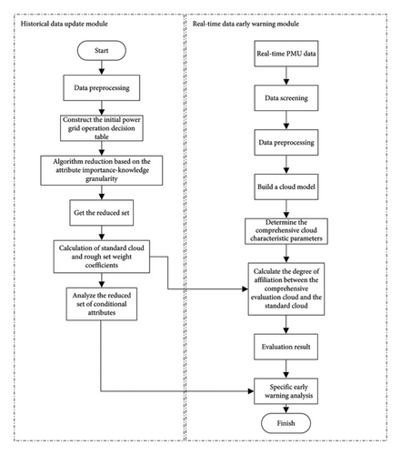
Step 1: Preprocessing data. We discretize the historical grid operation data according to the method in Section 3.1 to form a new set of objects U and build a new initial decision table S = {U, C, D, V, F}.
-
Step 2: The selection of condition attributes and decision attributes is carried out. This simulation is based on the general power system, the decision attribute is whether there is a fault in power grid, and the condition attribute set is the basic data indicator constructed in the above subsection.
-
Step 3: Build the power grid early warning information decision table, then use the reduction algorithm based on the attribute significance and knowledge granularity proposed in Section 3.2 to obtain the core attributes in the decision table, and calculate the weight wi for each conditional attribute based on ρ.
-
Step 4: After obtaining the attribute set of the simplified decision table, the comprehensive evaluation grade is constructed based on the core attributes therein according to the method in Section 3.5.1, and the cloud model feature parameters corresponding to the evaluation grade standard cloud are calculated according to the method in Section 3.3 by combining the data in the attribute set of the simplified conditions.
-
Step 5: Take out the PMU real-time data, calculate the comprehensive cloud evaluation results and the degree of affiliation, and finally derive the warning evaluation level according to the principle of maximum affiliation.
The framework of the specific early warning model algorithm is shown in Figure 3.
Overall, in terms of dimensionality simplification ability, compared with linear dimension reduction methods such as PCA, rough set eliminates redundant indicators while retaining key attributes with strong causal associations, ensuring that the indicator set still has clear power system physical meaning after dimension reduction. Meanwhile, the complexity of the rough set method is O(n), which is lower than the exponentially increasing complexity of local linear embedding (LLE) and other methods. Secondly, the cloud model updates the digital feature parameters in real time through the sliding window mechanism, so that the warning threshold can be dynamically adjusted with the load fluctuation of the grid. In terms of knowledge interpretability, the “conditional attribute-decision rule” generated by the rough set and the cloud model supports causal logic tracing, which is more suitable for the needs of grid operation and maintenance personnel for the transparency of the rules compared with the black-box models such as support vector machine (SVM) or deep learning.
4. Simulation and Verification
4.1. New England 10-Machine and 39-Node System Data Analysis
In order to illustrate and verify the effectiveness and feasibility of the algorithm in this paper, this paper selects the New England 10-machine and 39-node system for the simulation verification. The PMU dataset from New England 10-machine and 39-node, while reduced in scale, is highly representative of larger and more complex power system dataset. It has been widely adopted in power system studies due to its balance between simplicity and the inclusion of key operational and dynamic characteristics found in real-world grids. Although the New England 10-machine and 39-node system is a simplified model, its structure and behavior make it broadly applicable to larger systems, such as national or continental grids. The dynamic relationships between generators and loads, as well as the occurrence of faults and disturbances, are consistent with what is observed in more extensive grids. This makes the dataset an effective proxy for studying the behavior of larger systems, especially in terms of stability and fault response. For the warning and detection of LFO, the dataset offers a high level of completeness. It provides all the essential measurements (e.g., voltage, current, and frequency) that are required for identifying and diagnosing faults. The high-resolution and time-series data allow for both real-time fault detection and retrospective fault analysis, supporting the development of early warning systems. While the dataset does not capture all possible fault types or external environmental factors, its structured nature allows for fault scenarios to be simulated and analyzed in a controlled manner.
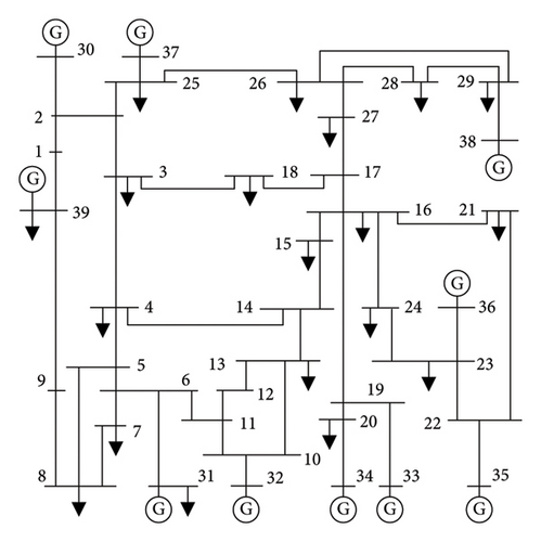
The data in this paper are selected from the PMU dataset of the New England 10-machine and 39-node system throughout the year, which has a sampling point every 15 min. A total of 35,040 data points throughout the year will be obtained, which is used as historical data for the correlation analysis. The dataset effectively captures essential system dynamics, which contains the frequency, phase shift, voltage, current, active and reactive power of each node, and so on. Then we selected August of that year as the test set to test the model effect, in which we selected 4 evaluation moments per day, for a total of 128 (T1–T128) evaluation moments in the whole month. The power system topology of the New England 10-machine and 39-node system constructed in this section is shown in Figure 4.
In this paper, MATLAB and Simulink simulation systems are used for experimental verification. A small load fluctuation (LFO) is applied to machine 5. The power and voltage values of the system are shown in Figure 5.
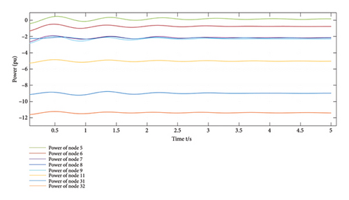
The operation of this simulation system shows that when the system undergoes LFOs, power fluctuations are generated in all lines 5–9, while small magnitude power oscillations are also generated in lines 11, 31, and 32. Then the system power fluctuation decreases and gradually tends to be stable. Compared with the total power before the LFO decreases, the system is damaged. But the LFO occurs rapidly and has the self-recovery nature, which is easy to cause the early warning system misjudgment, omission of judgment, and so on. The above phenomenon reflects that the early warning system should have the rapidity and accuracy of reflection, correctly reflecting the current power grid alarm, in order to carry out reasonable warning planning and avoid wasting resources.
4.2. Condition/Decision Attribute Selection and Data Discretization
When the power grid is running, the early warning indicators should be in line with the characteristics of the current power system model and can objectively reflect the operation state of power grid. Similarly, when selecting conditions or deciding attributes, the data processing advantages of rough set should also be adapted, and the indicators that can reflect the volatility and stability of the power grid should be selected as condition attributes.
The data are also discretized using the method in the previous section and categorized using the numbers 0, 1, and 2, where “0” indicates the indicator “normal”; “1” indicates the indicator “fluctuating”; and “2” indicates the indicator “deviating from normal values.” After discretization, the attribute values were compiled into a table of conditional attribute values as shown in Table 3.
| Indicator | Attribute |
|---|---|
| Bus start voltage | |
| Bus start current | |
| Bus voltage phase angle | |
| Bus current phase angle | |
| Unit active power | |
| Unit reactive power | |
| Unit frequency offset | |
| Unit oscillation amplitude ratio | |
| Unit dynamic damping ratio | |
| Unit power angle offset | |
| CΔP1∼3 | Power loss (zoning) |
| Transformer operating status | |
| Bus power | |
| CT | Ambient temperature |
| Cw | Ambient humidity |
4.3. Determination of Standard Cloud Parameters
The standard cloud parameters corresponding to the five warning levels calculated from historical grid data are shown in Table 4.
| Safety level | Cloud feature model parameters |
|---|---|
| I | (18, 9.52, 0.1) |
| II | (27, 6.18, 0.1) |
| III | (44, 5.70, 0.1) |
| IV | (62, 4.13, 0.1) |
| V | (91, 1.83,0.1) |
4.4. Approximation of Grid Conditional Attributes Based on Rough Set
Based on the historical operation data of the grid, a decision table is constructed, in which some of the conditional attributes corresponding to no fluctuations are reduced, and the decision table is shown in Table A1 in the Appendix (some samples are omitted).
The maximum importance reduction set {CPe} is taken as the initial reduction set, and its particle size entropy is calculated as I(D/CPe) = 0.187 ≠ I(D/C). Therefore, the remaining conditional attributes are added in sequence according to the comprehensive importance order SIG until the requirements are met, and the final reduced set is obtained, as shown in Table A2 in the Appendix.
4.5. Determination of Indicator Weights and Standard Cloud Parameters
Based on the approximated decision table, we obtain the core conditional attributes of the grid at this time, i.e., the filtered warning indicators, as shown in Table 5.
| Criterion layer | Indicator |
|---|---|
| Bus voltage | |
| Bus current | |
| Voltage phase angle | |
| Unit power | |
| Unit power angle offset | |
| Power loss | |
| Busbar power | |
| Unit frequency offset | |
| Dynamic damping ratio | |
| Unit oscillation amplitude ratio | |
Then we calculate the comprehensive cloud parameters and composite weights for each indicator based on the algorithm proposed in the previous section using the real-time PMU data (taking moment T97 as an example), and the specific values are shown in Table 6.
| Criterion layer | Criterion layer weight | Indicator | Weights | Characteristic parameters of cloud model | ||
|---|---|---|---|---|---|---|
| EX | En | He | ||||
| Bus voltage | 0.063 | 0.311 | 42.6 | 4.11 | 0.1 | |
| 0.689 | 72.3 | 4.54 | 0.1 | |||
| Bus current | 0.059 | 0.418 | 76.5 | 4.87 | 0.1 | |
| 0.582 | 52.4 | 4.50 | 0.1 | |||
| Voltage phase angle | 0.065 | 0.221 | 67.1 | 4.07 | 0.1 | |
| 0.396 | 64.6 | 2.83 | 0.1 | |||
| 0.383 | 90.9 | 1.42 | 0.1 | |||
| Unit power | 0.086 | 0.892 | 96.7 | 3.96 | 0.1 | |
| 0.108 | 99.1 | 1.83 | 0.1 | |||
| Unit power angle offset | 0.153 | 1 | 76.2 | 3.65 | 0.1 | |
| Power loss | 0.070 | 0.178 | 88.7 | 2.53 | 0.1 | |
| 0.622 | 57.4 | 3.14 | 0.1 | |||
| 0.200 | 54.8 | 2.70 | 0.1 | |||
| Busbar power | 0.02 | 0.686 | 79.5 | 2.68 | 0.1 | |
| 0.314 | 95.9 | 3.56 | 0.1 | |||
| Unit frequency offset | 0.164 | 1 | 72.1 | 1.15 | 0.1 | |
| Dynamic damping ratio | 0.138 | 1 | 58.8 | 2.71 | 0.1 | |
| Unit oscillation amplitude ratio | 0.182 | 1 | 43.5 | 1.98 | 0.1 | |
4.6. Evaluation of the Level of Early Warning Results
After obtaining the weights and integrated cloud parameters corresponding to each approximated grid indicator, the corresponding affiliation matrix Q is calculated according to the algorithm in Section 3.3, and finally the affiliations corresponding to different grid risk levels are obtained through equation (14) as shown in Table 7.
| Standard cloud | Cloud1 | Cloud2 | Cloud3 | Cloud4 | Cloud5 |
|---|---|---|---|---|---|
| Hazard degree | I | II | III | IV | V |
| Affiliation | 0.093 | 0.052 | 0.030 | 0.814 | 0.011 |
From Table 7, it can be seen that at this time the integrated evaluation of clouds corresponds to the largest affiliation of cloud 4, which indicates that the risk level of the grid at T97 is level IV, i.e., it may lead to a level 1 failure of the grid.
At the same time, we calculate the affiliation results for 128 moments corresponding to each risk, as shown in Figure 6.
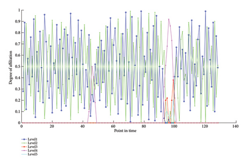
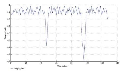
After obtaining the grid risk level affiliations corresponding to different time points, we calculate and test the grid damping ratios at different time points during the day, which is shown in Figure 7.
4.7. Analysis and Comparison of Results
According to Figure 7, it can be seen that the early warning assessment result of this paper’s method at the time of T97 is level IV, which may lead to a level I fault in the power grid. According to Figure 7, the corresponding risk level affiliation of the grid is level I or II most of the time, which becomes risk IV at T45 and T97 and has a tendency to develop into risk V at T98. Similarly, according to the analysis in Figure 7, the grid damping ratio decreases at time points T44 and T96, representing that the damping ratio is too low (close to zero), which indicates that the system is not sufficiently damped, and the system undergoes LFOs. It can be seen that the method in this paper successfully warns the LFO with low delay and high accuracy, which verifies the effectiveness of the method.
Then we, in order to further verify the effectiveness of the algorithm, take T90–T110 time points and compare the method of this paper with k-nearest neighbor (KNN), SVM, backpropagation (BP) neural network, and analytic hierarchy process (AHP) analysis method. The results are shown in Figure 8.

As can be seen from Figure 8, since the LFO starts at T95 and ends at T100, the method in this paper responds most rapidly and raises the warning evaluation level to 4 at the moment of T96, whereas all other methods suffer from the phenomenon of warning lag. Due to SVM method needing a lot of tuning parameters to assist, it fails to respond in time when the LFO occurs and delays the early warning time. The BP neural network method has some overfitting problems, which leads to premature judgment of early warning situation. Due to the lack of sufficient feature selection preprocessing ability, the KNN method misdetermines the occurrence time of LFO. Meanwhile, when the LFO disappears, the response speed of this paper’s method and the BP neural network method is the same, which adjusts the risk of LFO of the grid downward in time and reduces the waste of resources. However, the AHP method relies on the subjective judgment of weight and priority, and a large number of incomplete data information leads to the decline of the accuracy of its judgment matrix, which makes the AHP method misjudge the recovery time of LFO fault and reduce the warning level prematurely. Moreover, during the LFO, this paper’s method accurately predicts its risk degree as 4, but it does not rise to 5 (large-scale grid accidents), while other methods have different degrees of precision disorders. In summary, this paper’s method is superior to other methods in terms of warning response time and warning accuracy.
Meanwhile, to further compare the accuracy of this paper’s method, confusion matrix analysis is used, where the diagonal box represents that the actual risk matches the predicted risk, and the other boxes represent that the warning level and the real level do not match. The specific warning situation is shown in Figure 9.
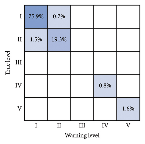
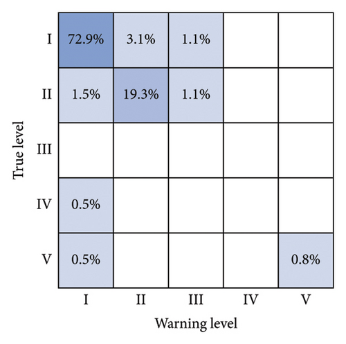
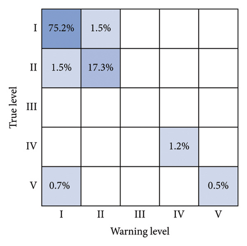
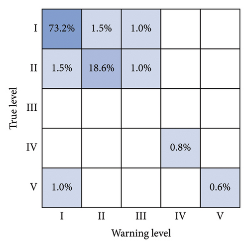
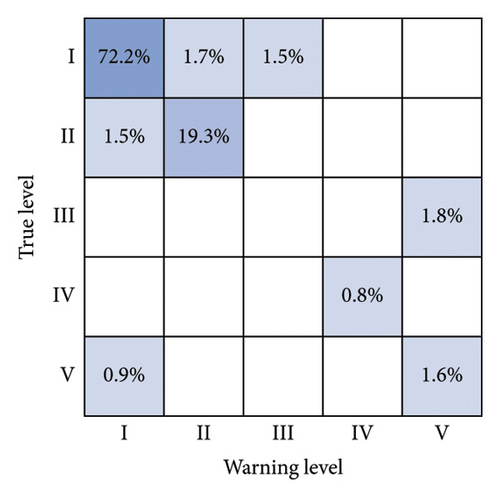
From the analysis of Figure 9, it can be seen that the proportion of samples represented by the diagonal box frame of this paper’s method is 75.9%, 19.3%, 0.8%, and 1.6%, respectively, which are higher than those of the other models, and the nondiagonal box frames of the other models still have different probabilities of appearing in the samples, which proves that this paper’s method is also ahead of the other methods in terms of accuracy.
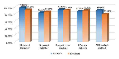
In order to further validate the advantages of the method in this paper, 128 assessment periods are compared with the real warning levels, and their precision and recall are calculated as shown in Figure 10. As can be seen from Figure 10, the accuracy and recall of the comprehensive warning model constructed by this paper’s method are above 90%. It is 15% points better than the KNN model with the lowest precision in the comparison of precision, and it is also slightly higher than that of the SVM method with stronger comprehensive performance, which once again verifies the effectiveness of this paper’s method.
To verify the effectiveness of the method in this paper, we collect historical fault data such as bus voltage and line power as a test set. Comparing the traditional statistical analysis methods, machine learning methods, etc., which include KNN method, SVM, and deep belief network (DBN) methods, the key performance indexes are given in Table 8.
| Methods | Average elapsed time (s) | Noise robustness (ΔAcc%) |
|---|---|---|
| Method of this paper | 0.92 | −2.6 |
| K-nearest neighbor method | 1.28 | −6.3 |
| SVM | 1.05 | −4.5 |
| DBN | 1.68 | −3.9 |
- Note: The significance of bold values given is to highlight the key performance results of using the proposed method of this paper.
From Table 8, it can be seen that the response speed and robustness of the methods in this paper are stronger than the statistical and machine learning methods; this is because the statistical methods often require a large number of parameter calculations, while the machine learning methods require training and GPU acceleration and also lead to poorer robustness due to their inability to recognize the physical significance of the attribute set.
In order to compare the contribution of this paper’s method with other methods in a more comprehensive way, we have selected some key performances of the early warning model for comparison, which are shown in Table 9.
| Method of this paper | K-nearest neighbor method | SVM | DBN | |
|---|---|---|---|---|
| False alarm rate | 5.9% | 8.6% | 6.7% | 6.2% |
| Feature dimension | 18 | 24 | 128 | 128 |
| Memory footprint | 640 MB | 792 MB | 3.2 GB | 2.4 GB |
| Number of interpretable rules | 23 | 8 | 0 | 0 |
| Parameter sensitivity | ±10% | ±22% | ±31% | ±42% |
The method proposed in this study achieves the synergistic optimization of accuracy, efficiency, and interpretability through the combination of rough sets and cloud models. Experiments show that under the premise that the false alarm rate (5.9%) is significantly lower than that of the traditional model (6.2%–8.6%), the feature dimension is compressed to 14%–23% of the comparative methods, and the memory occupation is only 26%–27% of that of the deep model (DBN/SVM), which breaks through the bottleneck of the lightweight deployment; at the same time, the method generates 23 interpretable rules, which is upgraded compared with the classical interpretable model (KNN) by 187.5%, which is the first time to realize the compatibility design between deep learning and symbolic reasoning, and solves the industry pain point of insufficient decision transparency in black-box models; in addition, the parameter sensitivity (±10%) is reduced by 54.5% compared with the optimal comparison model, which verifies the strengthening effect of algorithm robustness.
In discussion, the method in this paper is proved to be superior to mainstream methods in terms of warning accuracy and warning response speed. A new problem solving idea is proposed for the LFO warning problem, i.e., the use of rough sets to approximate the grid attributes and then the use of cloud models for comprehensive evaluation. Compared to the rough set method, the KNN method suffers from high sensitivity to noise and outliers, significant computational cost, scalability issues, and a lack of inherent feature selection. SVMs face high computational demands, complex parameter tuning, a risk of overfitting, and less interpretable decision boundaries. BP neural networks are challenged by long training times, overfitting, interpretability issues due to their black-box nature, and sensitivity to hyperparameters. The AHP is hindered by subjectivity in judgments, complexity in managing large systems, and potential inconsistencies. In contrast, the rough set method excels in early warning systems by effectively handling uncertainty and incomplete information, providing clear and interpretable decision rules, and offering a robust framework for feature selection without the need for prior knowledge of the data distribution. At present, this study still contains some limitations in computational processing, and future research work should be carried out in simplifying computational processing and reducing computational complexity.
While the rough set method offers significant benefits for early warning systems, it also has limitations that require critical examination. One key limitation is its susceptibility to potential biases based on the quality and representativeness of the data used. If the dataset contains biases or lacks representation of all possible scenarios, the decision rules derived may not be universally applicable or may miss important patterns. Additionally, the method faces scalability challenges as the size and complexity of the data grow. Larger grid systems or datasets with many features can lead to significant computational effort and may impact the method’s performance due to the increased number of possible rules and their interactions. Furthermore, rough sets may struggle with capturing complex, nonlinear relationships within the data, which can limit their accuracy in providing early warnings in systems where such relationships are critical. The generation of decision rules can also lead to rule overload, where managing and interpreting a large number of rules become cumbersome, potentially diminishing the effectiveness of the early warning system. Addressing these limitations involves refining the rough set approach to improve scalability, ensuring data quality and representativeness, and possibly integrating it with other methods to capture complex relationships and enhance overall performance.
5. Conclusion
Future research can continue to advance along the explicit technical paradigm of this paper: the rough set–cloud model hybrid warning architecture constructed in this paper opens up a new methodological path for power system fault warning. Compared with the neural network relying on black-boxed weights and the KNN method with response hysteresis, this study achieves the synergistic optimization of response efficiency and recall rate through the attribute importance-knowledge granularity weight allocation mechanism while ensuring the transparency of the warning logic; the core breakthrough of this study lies in ① small sample adaptability—a dynamic approximation strategy designed for the residual historical data and high-dimensional characteristics of real-time information, which significantly reduces the model’s dependence on data size; ② physical interpretability—The comprehensive evaluation system based on cloud modeling maps implicit features into explicit rule clusters, overcoming the shortcomings of traditional data-driven methods with fuzzy decision basis; and ③ lightweight reasoning—compression of redundant computation through feature space reconstruction to provide underlying architectural support for edge-side real-time warning. These findings point out the hybrid design direction of fusing symbolic reasoning and data intelligence for the next-generation electric power security prevention and control system, and the subsequent exploration can focus on three major derivative scenarios: expanding the adaptive fusion capability of multisource heterogeneous data based on this architecture, developing an online learning mechanism for the dynamic grid environment, and constructing a collaborative decision-making framework for the big model of artificial intelligence and the knowledge-approximation engine. This study verifies the engineering potential of rough set theory in power critical tasks, and its characteristics of “low dependence, high transparency, and fast response” are expected to reshape the fault warning technology system of new energy-dominated power grids.
Conflicts of Interest
The authors declare no conflicts of interest.
Funding
This work was supported in part by Natural Science Foundation of Beijing Municipal under grant no. 4242035, in part by Shandong University Key Laboratory of Power System Intelligent Dispatch and Control, Ministry of Education, and in part by National Natural Science Foundation of China under grant no. 51407201.
Appendix A: The Formulas Omitted in This Paper
Definition 1. Knowledge granularity: In the knowledge base S = (U, R), the division of knowledge R on the domain U can be expressed as U/R = {R1, R2, R3, …, Rn}, and we use GD(R) to represent the granularity of knowledge R, marking the resolution of R as Dis(R) = 1 − GD(R). Therefore, we have
As we know, the larger the GD(R) is, the smaller the Dis(R) will be, where card(U) is the base quantity of set U.
Definition 2. Let U/R = {R1, R2, R3, …, Rn} be knowledge on the domain U; then the granularity entropy of knowledge is defined as
Definition 3. In an information system S = {U, C, D, V, F}, U represents all domains; C represents a nonempty finite set of attributes; V represents the range of each attribute; and x is an attribute in the attribute subset U ∈ C. The importance of x to X is the improvement of X resolution after x is increased. The more resolution increases, the more important x will be to X. The importance of x to X is denoted as Sigx(X), calculated by the following formula [21].
Definition 4. Let U be a numerical domain of theory, where X represents a qualitative concept of U. If the quantitative value x ∈ U and x is a one-time random implementation of the qualitative concept X, X will have the stable propensity randomness for the certainty μx(x) ∈ [0, 1] of the qualitative concept x. If μ : U⟶[0, 1], ∀x ∈ U, x⟶U(x), then the distribution of x in U is said to be a cloud model, or cloud for short, where each x becomes a cloud droplet.
| ⋱ | ||||||||||||||||||||||
|---|---|---|---|---|---|---|---|---|---|---|---|---|---|---|---|---|---|---|---|---|---|---|
| 1 | 0 | 0 | 1 | 0 | 0 | 1 | 0 | 1 | 1 | 1 | 1 | 1 | 1 | 1 | 1 | 1 | 1 | 1 | 1 | 1 | 1 | 1 |
| 2 | 0 | 0 | 1 | 1 | 1 | 0 | 0 | 0 | 0 | 0 | 0 | 0 | 0 | 0 | 0 | 0 | 0 | 0 | 0 | 0 | 0 | 0 |
| 3 | 0 | 1 | 1 | 0 | 1 | 0 | 0 | 1 | 0 | 0 | 0 | 1 | 0 | 0 | 0 | 2 | 0 | 0 | 0 | 0 | 0 | 0 |
| 4 | 0 | 0 | 0 | 1 | 0 | 1 | 0 | 1 | 1 | 0 | 0 | 1 | 0 | 0 | 0 | 1 | 0 | 0 | 0 | 0 | 0 | 0 |
| 5 | 1 | 0 | 1 | 1 | 0 | 2 | 0 | 2 | 0 | 0 | 0 | 0 | 2 | 0 | 2 | 2 | 0 | 0 | 0 | 0 | 0 | 0 |
| 6 | 0 | 0 | 0 | 0 | 1 | 1 | 0 | 0 | 2 | 0 | 0 | 0 | 0 | 0 | 0 | 0 | 0 | 0 | 0 | 0 | 0 | 1 |
| 7 | 0 | 1 | 0 | 1 | 1 | 0 | 0 | 2 | 2 | 0 | 0 | 0 | 0 | 0 | 0 | 0 | 0 | 0 | 0 | 0 | 0 | 0 |
| 8 | 0 | 0 | 1 | 0 | 0 | 1 | 0 | 1 | 1 | 1 | 1 | 1 | 1 | 1 | 1 | 1 | 1 | 1 | 1 | 1 | 1 | 0 |
| 9 | 1 | 0 | 1 | 0 | 1 | 0 | 0 | 0 | 0 | 0 | 0 | 0 | 0 | 0 | 0 | 2 | 0 | 0 | 0 | 0 | 0 | 0 |
| 10 | 0 | 1 | 1 | 0 | 1 | 0 | 0 | 1 | 1 | 0 | 0 | 2 | 0 | 0 | 0 | 2 | 0 | 0 | 0 | 0 | 0 | 0 |
| 11 | 0 | 0 | 0 | 2 | 0 | 1 | 1 | 0 | 1 | 0 | 0 | 2 | 1 | 0 | 0 | 2 | 0 | 2 | 0 | 0 | 0 | 2 |
| 12 | 1 | 0 | 1 | 1 | 0 | 0 | 0 | 1 | 2 | 0 | 0 | 0 | 0 | 0 | 0 | 1 | 0 | 0 | 0 | 0 | 2 | 0 |
| 13 | 0 | 0 | 0 | 0 | 1 | 2 | 0 | 1 | 0 | 0 | 0 | 1 | 1 | 0 | 1 | 0 | 1 | 0 | 0 | 0 | 0 | 0 |
| 14 | 0 | 0 | 0 | 0 | 1 | 1 | 0 | 1 | 0 | 0 | 0 | 1 | 0 | 0 | 0 | 1 | 0 | 0 | 0 | 0 | 0 | 0 |
| 15 | 0 | 0 | 0 | 2 | 1 | 0 | 0 | 1 | 0 | 0 | 0 | 0 | 2 | 0 | 0 | 1 | 0 | 0 | 0 | 0 | 0 | 0 |
| 16 | 0 | 0 | 0 | 0 | 1 | 1 | 0 | 0 | 0 | 0 | 0 | 0 | 0 | 0 | 0 | 0 | 0 | 0 | 0 | 0 | 1 | 1 |
| 17 | 0 | 0 | 0 | 0 | 1 | 1 | 0 | 0 | 1 | 0 | 0 | 1 | 1 | 0 | 0 | 0 | 0 | 0 | 0 | 0 | 0 | 0 |
| 18 | 0 | 0 | 0 | 1 | 1 | 1 | 0 | 0 | 1 | 0 | 0 | 0 | 0 | 0 | 0 | 1 | 0 | 0 | 0 | 0 | 0 | 0 |
| ⋮ | ⋯ | ⋯ | ⋯ | ⋯ | ⋯ | ⋯ | ⋯ | ⋯ | ⋯ | ⋯ | ⋯ | ⋯ | ⋯ | ⋯ | ⋯ | ⋯ | ⋯ | ⋯ | ⋯ | ⋯ | ⋯ | ⋯ |
| 50 | 0 | 0 | 0 | 0 | 1 | 1 | 0 | 2 | 1 | 0 | 0 | 1 | 1 | 0 | 0 | 2 | 0 | 0 | 0 | 2 | 0 | 1 |
| ⋱ | ||||||||||||||||||||||
| 1 | 0 | 0 | 1 | 0 | 0 | 1 | 0 | 0 | 1 | 1 | 1 | 1 | 1 | 1 | 1 | 1 | 1 | 1 | 1 | 1 | 1 | 1 |
| 2 | 1 | 0 | 1 | 0 | 1 | 0 | 0 | 0 | 0 | 0 | 0 | 0 | 0 | 0 | 0 | 0 | 0 | 1 | 0 | 1 | 0 | 0 |
| 3 | 1 | 1 | 1 | 0 | 1 | 0 | 0 | 0 | 0 | 0 | 0 | 0 | 0 | 0 | 0 | 0 | 0 | 0 | 1 | 0 | 1 | 0 |
| 4 | 0 | 0 | 0 | 1 | 0 | 1 | 0 | 0 | 1 | 0 | 0 | 0 | 0 | 1 | 0 | 0 | 0 | 1 | 1 | 0 | 0 | 0 |
| 5 | 1 | 0 | 1 | 1 | 0 | 0 | 0 | 0 | 0 | 0 | 0 | 0 | 0 | 0 | 0 | 0 | 0 | 0 | 0 | 1 | 0 | 0 |
| 6 | 0 | 0 | 0 | 0 | 1 | 0 | 0 | 0 | 0 | 0 | 0 | 0 | 0 | 0 | 1 | 0 | 0 | 0 | 1 | 1 | 1 | 0 |
| 7 | 0 | 0 | 0 | 1 | 1 | 1 | 0 | 0 | 0 | 0 | 0 | 0 | 0 | 0 | 0 | 0 | 0 | 2 | 0 | 0 | 2 | 1 |
| 8 | 0 | 0 | 2 | 0 | 0 | 2 | 1 | 1 | 1 | 1 | 0 | 0 | 1 | 1 | 1 | 1 | 1 | 2 | 1 | 1 | 0 | 0 |
| 9 | 1 | 0 | 2 | 1 | 1 | 0 | 0 | 0 | 0 | 0 | 0 | 0 | 0 | 0 | 0 | 0 | 0 | 1 | 0 | 1 | 0 | 0 |
| 10 | 0 | 1 | 1 | 0 | 0 | 0 | 0 | 0 | 0 | 0 | 0 | 0 | 0 | 1 | 0 | 0 | 0 | 0 | 0 | 0 | 0 | 0 |
| 11 | 0 | 0 | 1 | 0 | 0 | 1 | 0 | 0 | 0 | 0 | 0 | 0 | 0 | 0 | 0 | 0 | 0 | 0 | 0 | 0 | 0 | 0 |
| 12 | 1 | 0 | 1 | 0 | 0 | 0 | 0 | 1 | 0 | 0 | 0 | 0 | 1 | 1 | 0 | 1 | 0 | 0 | 0 | 0 | 0 | 0 |
| 13 | 0 | 1 | 0 | 0 | 1 | 1 | 0 | 1 | 0 | 0 | 0 | 0 | 1 | 0 | 1 | 1 | 0 | 0 | 1 | 1 | 0 | 1 |
| 14 | 0 | 0 | 0 | 0 | 1 | 0 | 1 | 0 | 1 | 0 | 0 | 0 | 0 | 0 | 0 | 0 | 0 | 0 | 1 | 0 | 1 | 0 |
| 15 | 0 | 0 | 2 | 0 | 0 | 0 | 0 | 0 | 0 | 0 | 0 | 0 | 1 | 0 | 0 | 1 | 0 | 0 | 0 | 0 | 0 | 0 |
| 16 | 0 | 0 | 1 | 0 | 1 | 0 | 0 | 0 | 0 | 0 | 0 | 0 | 1 | 1 | 0 | 1 | 0 | 0 | 1 | 0 | 0 | 0 |
| 17 | 0 | 0 | 0 | 1 | 0 | 1 | 0 | 0 | 0 | 0 | 0 | 0 | 0 | 0 | 0 | 0 | 0 | 0 | 1 | 1 | 0 | 1 |
| 18 | 0 | 0 | 0 | 0 | 0 | 1 | 0 | 0 | 0 | 0 | 0 | 0 | 0 | 0 | 0 | 0 | 0 | 0 | 0 | 0 | 0 | 0 |
| ⋮ | ⋯ | ⋯ | ⋯ | ⋯ | ⋯ | ⋯ | ⋯ | ⋯ | ⋯ | ⋯ | ⋯ | ⋯ | ⋯ | ⋯ | ⋯ | ⋯ | ⋯ | ⋯ | ⋯ | ⋯ | ⋯ | ⋯ |
| 50 | 0 | 0 | 1 | 0 | 1 | 1 | 0 | 0 | 0 | 0 | 0 | 0 | 0 | 0 | 0 | 0 | 0 | 0 | 0 | 0 | 0 | 0 |
| ⋱ | C24 | CT | D | |||||||||||||||||||
| 1 | 1 | 1 | 0 | 1 | 0 | 1 | 0 | 1 | 1 | 1 | 1 | 1 | 1 | 1 | 1 | 1 | 1 | 1 | 1 | 1 | 1 | D1 |
| 2 | 1 | 0 | 1 | 1 | 1 | 0 | 0 | 0 | 1 | 0 | 1 | 0 | 0 | 0 | 0 | 0 | 0 | 0 | 0 | 0 | 0 | D1 |
| 3 | 0 | 0 | 0 | 0 | 1 | 0 | 0 | 1 | 1 | 0 | 0 | 0 | 0 | 1 | 0 | 0 | 0 | 0 | 0 | 0 | 0 | D1 |
| 4 | 1 | 0 | 0 | 1 | 0 | 1 | 0 | 0 | 0 | 1 | 0 | 0 | 1 | 0 | 0 | 1 | 0 | 0 | 0 | 0 | 0 | D1 |
| 5 | 1 | 0 | 1 | 1 | 0 | 0 | 0 | 0 | 1 | 1 | 1 | 0 | 0 | 0 | 0 | 1 | 0 | 0 | 0 | 0 | 0 | D1 |
| 6 | 0 | 0 | 0 | 0 | 1 | 1 | 0 | 0 | 0 | 0 | 0 | 0 | 0 | 2 | 0 | 0 | 0 | 0 | 0 | 0 | 0 | D1 |
| 7 | 0 | 1 | 0 | 1 | 1 | 0 | 0 | 0 | 0 | 0 | 0 | 0 | 0 | 1 | 0 | 1 | 0 | 0 | 0 | 0 | 0 | D2 |
| 8 | 0 | 0 | 1 | 0 | 0 | 1 | 0 | 1 | 1 | 1 | 1 | 1 | 1 | 1 | 1 | 1 | 1 | 1 | 1 | 1 | 1 | D2 |
| 9 | 1 | 0 | 1 | 0 | 1 | 0 | 0 | 0 | 0 | 0 | 0 | 0 | 0 | 0 | 0 | 0 | 0 | 0 | 0 | 0 | 0 | D2 |
| 10 | 1 | 1 | 1 | 0 | 1 | 0 | 0 | 0 | 0 | 0 | 0 | 0 | 0 | 0 | 0 | 0 | 0 | 0 | 0 | 0 | 0 | D2 |
| 11 | 0 | 0 | 0 | 1 | 0 | 1 | 0 | 0 | 0 | 0 | 0 | 0 | 0 | 1 | 0 | 0 | 0 | 0 | 0 | 0 | 0 | D3 |
| 12 | 1 | 0 | 1 | 1 | 0 | 0 | 0 | 0 | 0 | 0 | 0 | 0 | 1 | 0 | 0 | 1 | 0 | 0 | 0 | 0 | 0 | D3 |
| 13 | 0 | 0 | 0 | 0 | 1 | 0 | 1 | 0 | 0 | 0 | 0 | 0 | 0 | 0 | 0 | 1 | 0 | 0 | 0 | 0 | 0 | D3 |
| 14 | 0 | 0 | 0 | 0 | 1 | 1 | 0 | 0 | 1 | 0 | 0 | 0 | 0 | 2 | 0 | 0 | 0 | 0 | 0 | 1 | 0 | D3 |
| 15 | 0 | 0 | 0 | 0 | 1 | 0 | 0 | 0 | 1 | 0 | 0 | 0 | 0 | 1 | 0 | 1 | 0 | 0 | 1 | 0 | 0 | D3 |
| 16 | 0 | 0 | 0 | 0 | 1 | 0 | 2 | 0 | 0 | 0 | 0 | 0 | 0 | 0 | 0 | 0 | 0 | 1 | 0 | 0 | 1 | D3 |
| 17 | 0 | 0 | 0 | 0 | 1 | 0 | 1 | 0 | 1 | 0 | 0 | 0 | 0 | 0 | 0 | 0 | 0 | 0 | 0 | 0 | 1 | No |
| 18 | 0 | 0 | 0 | 0 | 1 | 1 | 0 | 0 | 0 | 0 | 0 | 0 | 0 | 0 | 0 | 0 | 0 | 0 | 2 | 0 | 0 | No |
| ⋮ | ⋯ | ⋯ | ⋯ | ⋯ | ⋯ | ⋯ | ⋯ | ⋯ | ⋯ | ⋯ | ⋯ | ⋯ | ⋯ | ⋯ | ⋯ | ⋯ | ⋯ | ⋯ | ⋯ | ⋯ | ⋯ | ⋯ |
| 50 | 0 | 0 | 0 | 0 | 1 | 1 | 0 | 0 | 0 | 0 | 0 | 0 | 0 | 0 | 0 | 0 | 0 | 0 | 0 | 0 | 0 | No |
| ⋱ | D | |||||||||||||||||||
|---|---|---|---|---|---|---|---|---|---|---|---|---|---|---|---|---|---|---|---|---|
| 1 | 0 | 0 | 1 | 1 | 1 | 1 | 1 | 1 | 1 | 1 | 1 | 1 | 1 | 1 | 1 | 1 | 1 | 1 | 1 | D1 |
| 2 | 1 | 1 | 0 | 0 | 0 | 0 | 0 | 0 | 0 | 0 | 0 | 1 | 0 | 0 | 0 | 1 | 0 | 0 | 0 | D1 |
| 3 | 0 | 1 | 0 | 0 | 1 | 0 | 2 | 0 | 0 | 0 | 0 | 0 | 1 | 0 | 1 | 1 | 0 | 0 | 0 | D1 |
| 4 | 1 | 0 | 1 | 0 | 1 | 0 | 1 | 0 | 1 | 0 | 0 | 1 | 1 | 0 | 0 | 0 | 1 | 0 | 1 | D1 |
| 5 | 1 | 0 | 0 | 0 | 0 | 2 | 2 | 0 | 0 | 0 | 0 | 0 | 0 | 0 | 0 | 1 | 1 | 0 | 1 | D1 |
| 6 | 0 | 1 | 2 | 0 | 0 | 0 | 0 | 1 | 0 | 0 | 0 | 0 | 1 | 0 | 0 | 0 | 0 | 0 | 0 | D1 |
| 7 | 1 | 1 | 2 | 0 | 0 | 0 | 0 | 0 | 1 | 0 | 0 | 2 | 0 | 1 | 0 | 0 | 0 | 0 | 1 | D2 |
| 8 | 0 | 0 | 1 | 1 | 1 | 1 | 1 | 0 | 2 | 1 | 0 | 2 | 1 | 0 | 1 | 1 | 1 | 1 | 1 | D2 |
| 9 | 0 | 1 | 0 | 0 | 0 | 0 | 2 | 0 | 0 | 0 | 0 | 1 | 0 | 0 | 0 | 0 | 0 | 0 | 0 | D2 |
| 10 | 0 | 1 | 1 | 0 | 2 | 0 | 2 | 0 | 0 | 0 | 0 | 0 | 0 | 1 | 0 | 0 | 0 | 0 | 0 | D2 |
| 11 | 2 | 0 | 1 | 0 | 2 | 1 | 2 | 2 | 1 | 0 | 0 | 0 | 0 | 0 | 0 | 0 | 0 | 0 | 0 | D3 |
| 12 | 1 | 0 | 2 | 0 | 0 | 0 | 1 | 0 | 0 | 0 | 0 | 0 | 0 | 0 | 0 | 0 | 0 | 0 | 1 | D3 |
| 13 | 0 | 1 | 0 | 0 | 1 | 1 | 0 | 0 | 1 | 0 | 0 | 0 | 1 | 0 | 0 | 0 | 0 | 0 | 1 | D3 |
| 14 | 0 | 1 | 0 | 0 | 1 | 0 | 1 | 0 | 0 | 0 | 0 | 0 | 1 | 0 | 0 | 1 | 0 | 0 | 0 | D3 |
| 15 | 2 | 1 | 0 | 0 | 0 | 2 | 1 | 0 | 0 | 0 | 0 | 0 | 0 | 0 | 0 | 1 | 0 | 0 | 1 | D3 |
| ⋮ | ⋯ | ⋯ | ⋯ | ⋯ | ⋯ | ⋯ | ⋯ | ⋯ | ⋯ | ⋯ | ⋯ | ⋯ | ⋯ | ⋯ | ⋯ | ⋯ | ⋯ | ⋯ | ⋯ | ⋯ |
| 50 | 0 | 1 | 1 | 0 | 1 | 1 | 2 | 1 | 1 | 0 | 0 | 0 | 0 | 0 | 0 | 0 | 0 | 0 | 0 | No |
Open Research
Data Availability Statement
The data of this paper is openly available in [IEEE Dataport] at https://doi.org/10.21227/vkz3-2e96., reference number [Matija Naglic, 2019. PMU measurements of IEEE 39-bus power system model].


