Sustainable Electric Railway System Integrated With Distributed Energy Resources: Optimal Operation and Smart Energy Management System
Abstract
Global concern about the energy crisis and its environmental impact has focused on sustainable alternatives. The electric railway system (ERS) is a major electrical energy consumer, contributing to greenhouse gas (GHG) emissions and CO2 pollution. This study introduces railway energy management systems (REMSs) as a green solution to address these challenges. REMS not only mitigates environmental risks but also enables surplus electricity sales to the grid market. This research formulates an AC optimal power flow (AC-OPF) problem by the utilization of mixed integer linear programming (MILP) for optimization of the railway station electrical system operation cost. In this paper, renewable energy resources (RERs), energy storage systems (ESSs), and regenerative braking energy (RBE) are taken into account, as well as the electrical grid. Additionally, by considering the probabilistic and stochastic behaviors of RERs, ESSs, and RBE, using real-time data, significant cost reductions in the daily operations of smart railway stations are achieved. With the aid of MATLAB, the model is effectively solved, and the results provide compelling evidence of the suitability and remarkable effectiveness of the proposed model.
1. Introduction
The proliferation of vehicles has led to a multitude of pressing problems, notably the detrimental impact of air and noise pollution [1]. Indeed, reports indicate that transportation accounts for approximately 14% of total GHG emissions as of 2010, with projections indicating a doubling of this figure by 2050 [2]. Furthermore, the rapid expansion of both population and industries has fueled an escalating demand for extensive transportation networks [3]. Transportation alone is responsible for a staggering 23.4% of global carbon emissions [4].
Railway stations are significant structures that consume a substantial amount of energy. This energy consumption is primarily attributed to the trains themselves, which require significant power to operate and move efficiently. To address this issue and promote sustainability, it is crucial to prioritize the development of clean and renewable energy sources as alternatives to fossil fuels. Additionally, the establishment of distributed smart energy stations can play a pivotal role in providing renewable cold, heat, power, and water to new buildings, thereby significantly reducing their energy consumption to ultralow or zero levels [5]. In the context of smart high-speed railway stations, there exists an opportunity for enhanced energy efficiency such as:
Trajectory optimization: Implementing advanced algorithms to optimize the trajectory of individual metro trains can significantly reduce energy consumption. By considering factors such as train speed, acceleration, and braking, it is possible to minimize energy wastage and improve overall efficiency [6–8].
Optimized timetables: Developing optimized timetables for traction substations in railway systems can help streamline energy usage. By coordinating train schedules with the availability and capacity of substations, it is possible to reduce energy waste and improve the overall utilization of resources [9, 10].
Power electronics and energy storage: Utilizing power electronic devices, such as regenerative braking (RB) systems, can capture and store energy that would otherwise be wasted during braking. Additionally, incorporating wayside ESS allows for efficient distribution and utilization of energy across the railway network. Integrating renewable energy generation sources, such as solar or wind, further reduces reliance on traditional power sources and promotes sustainability [11, 12].
By implementing these technologies, railway stations can become self-sufficient in meeting their energy needs while also contributing to the overall sustainability goals of the transportation sector.
Smart railway energy management system is one of the greenest, most modern, and eco-friendly techniques which optimizes energy usage and enhances efficiency in railway stations. As REMS is based on smart grid concepts [13], it can integrate with various railway components, using advanced technologies to monitor and control energy consumption. Real-time data analysis and intelligent algorithms minimize wastage, reduce emissions, and lower costs. The system enables load balancing, RB, and smart power distribution, improving sustainability and reliability.
The development and implementation of an effective control strategy play a pivotal role in the success of any system [14, 15]. In the context of enhancing energy efficiency in electrical railway systems by storing RBE in ESSs, various control strategies have been proposed [16]. These strategies outline the utilization of ESS applications such as batteries, flywheels, and electric double-layer capacitors. By employing these strategies, the aim is to optimize the storage and utilization of RBE, leading to improved overall system performance [17].
A basic REMS is implemented in [18]. ESSs, such as batteries, are charged during low-demand periods (such as nighttime when electricity tariffs are low) using the primary grid. Additionally, PV panels installed in the station store energy on ESSs during peak sunlight hours around noon at no cost. These ESSs are then discharged into the station grid during high-demand hours, resulting in notable cost reductions for electricity consumption.
Integrating ERSs and electric vehicle charging stations (EVChSs) at significant locations, such as parking areas near ERS stations or rail transport intermodal terminals, while effectively utilizing trains’ RBE as an additional power source, has the potential to enhance energy efficiency in EVChSs and decrease costs [19–23]. In [24], a comprehensive power management system is introduced, which incorporates RBE to integrate wind, solar, and electric vehicle (EV) charging infrastructures into MVDC railway microgrids. In [25], a modeling study was conducted on a region that included a metro system, EVs, and distributed generation. The focus was on determining the optimal utilization of RBE generated by the metro system to power other trains or EVs.
In [26], an optimal energy management strategy is proposed, employing the MILP method. The strategy utilizes the existing installed capacity of the rail system for service and transportation purposes, while also considering the integration of RBE and ESS. Additionally, a photovoltaic (PV) generation unit situated in the parking area is utilized to meet the energy demand of the EVs parking area, including the charging spaces for EVs and electric buses.
A stochastic approach is employed to develop a heuristic MILP model for energy management in railway stations in [27]. The model is designed to effectively generate RBE during braking to power various station loads. Additionally, the paper proposes a REMS model, which incorporates an ESS, RBE utilization, a solar PV generator, and an external grid to further optimize energy usage and enhance overall efficiency.
Evolutionary algorithms (EAs) have found wide-ranging applications in numerous engineering domains [28–31], as well as railways [32]. The authors of [33] implement differential evolution algorithm (DEA) to model REMS including renewable energy resources (RERs) (wind and solar PV systems), RB capabilities, and hybrid energy storage to minimizing the railway station operational cost. Also, the author of [34] applies nonlinear programming (NLP) and the DEA, a meta-heuristic method, to develop a REMS. The REMS incorporates renewable resources, ESSs, and RBE to minimize the overall cost of the station.
The authors of [35] suggest an ERS that employs clustering algorithms to achieve efficient stochastic energy management. This system aims to tackle the challenges associated with EMSs and make use of RBE to minimize the production cost of power plants in the upstream power system, which provides energy to the integrated energy systems.
In [36], the authors introduced a stochastic biobjective model that relies on a structural model of a multienergy hub system. The goal is to minimize operational costs and carbon emissions in a smart railway station and its associated commercial buildings. The energy hub system (EHS) consists of three subenergy hubs: one for power, one for heating, and one for cooling. Notably, the energy generated from RB during train deceleration is harnessed to power the EHS.
A new configuration for power optimization controllers is introduced in [37], comprising two distinct approaches: a higher-level strategy and a lower-level strategy. The higher-level strategy oversees the energy flow within the substation, while the lower-level strategy manages the power distribution within the hybrid energy storage system (HESS). To address the optimization challenge, a MILP approach is utilized. This method considers the operational discrepancies of electric multiple units (EMUs) and PV panels, ultimately reducing costs associated with operation and management.
In [38], the focus is on energy management for cophase traction substations (CTSSs) with the objective of minimizing operating expenses. This is achieved by coordinating various elements such as PV systems, HESS, power flow controllers (PFCs), and energy exchanges with the power grid. The authors specifically address the constraint of three-phase voltage imbalance. The energy management process consists of two stages: Stage I involves determining the operating status of the HESS and the energy transactions with the grid, while Stage II identifies the worst-case scenario that results in the highest operating costs for the CTSS. To solve this optimization problem, MILP is employed, using an efficient algorithm based on column-and-constraint generation.
In [39], it is suggested that smart rail systems (SRSs) can be operated optimally through the use of probabilistic clustering. The SRS structures demonstrate their ability to exchange energy with the utility grid and participate in the daily power market. To ensure optimal operation, an EMS controls the SRS. The EMS utilizes historical data, technical specifications of components, and power demand to calculate the required power exchange with the utility grid.
Table 1 provides a comprehensive comparison of the studies mentioned in the literature. This detailed analysis has contributed to a deeper understanding of the existing gaps in the research field.
| Ref | Year | Optimization method | Research concern elements | Stochastic behavior | |||||||
|---|---|---|---|---|---|---|---|---|---|---|---|
| PV | Wind | RBE | ESS | Pricing scheme | PV | Wind | RBE | ESS | |||
| [26] | 2022 | MILP | ✓ | ⨯ | ✓ | ✓ | ✓ | ✓ | ⨯ | ✓ | ✓ |
| [27] | 2018 | Heuristic MILP | ✓ | ⨯ | ✓ | ✓ | ✓ | ✓ | ⨯ | ✓ | ✓ |
| [33] | 2019 | DEA | ✓ | ✓ | ✓ | ✓ | ✓ | ✓ | ✓ | ⨯ | ✓ |
| [34] | 2021 | NLP/DEA | ✓ | ✓ | ✓ | ✓ | ✓ | ✓ | ✓ | ⨯ | ✓ |
| [35] | 2022 | MCS | ✓ | ✓ | ✓ | ✓ | ⨯ | ✓ | ✓ | ⨯ | ✓ |
| [36] | 2021 | DRP/MILP | ✓ | ⨯ | ✓ | ✓ | ⨯ | ✓ | ⨯ | ✓ | ⨯ |
| [37] | 2020 | MILP | ✓ | ⨯ | ✓ | ✓ | ✓ | ⨯ | ⨯ | ⨯ | ⨯ |
| [38] | 2022 | MILP/C&CG | ✓ | ⨯ | ⨯ | ✓ | ⨯ | ✓ | ⨯ | ⨯ | ⨯ |
| [39] | 2022 | MCS | ✓ | ⨯ | ✓ | ✓ | ✓ | ✓ | ⨯ | ✓ | ⨯ |
| This study | 2023 | MILP | ✓ | ✓ | ✓ | ✓ | ✓ | ✓ | ✓ | ✓ | ✓ |
- •
Introduction of a novel MILP model for REMS based on the smart grid architecture concept.
- •
Incorporation of various components including ESS and RER such as PV and wind turbines (WTs), RBE, and different pricing schemes for the first time in the literature.
- •
Utilization of a stochastic programming approach to evaluate the operation of a railway station, considering the uncertainty associated with the initial state of energy (SOE) of ESS, PV generation, wind generation, and the stochastic behavior of RBE based on the daily passenger profile.
- •
Consideration of different pricing signals throughout the day to fulfill the stochastic behavior of the grid.
- •
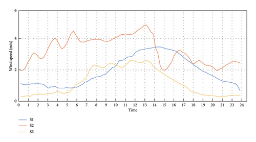
Examination of the probabilistic behavior of renewable resources and ESSs, taking into account the likelihood of ESS state, solar irradiation, and wind speed on a per-minute basis.
- •
Comprehensive assessment of the operational performance of the railway station in the presence of uncertain and variable RER.
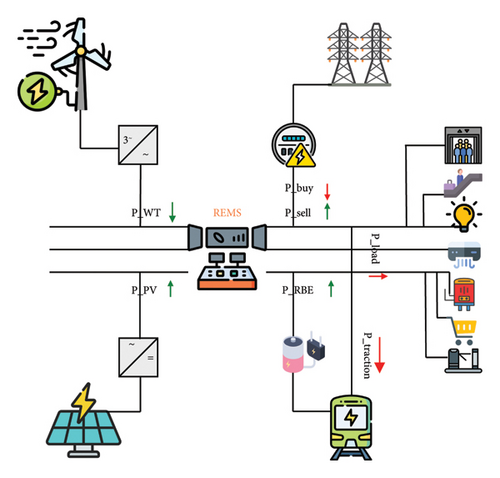
The block diagram of proposed REMS is illustrated in Figure 1. The study focuses solely on the internal energy demand of a railway station, with the assumption that the energy required for train operations is supplied through traction transformers. Designing optimal sizes of the interfacing converters [40] is one of the other aspects of smart railway systems which is our primary focus in this paper that is out of scope of our primary focus in this paper.
The rest of the paper is organized as follows: methodology and mathematics are given in Section 3. In Section 4, the different case studies and results are expressed. Finally, the concluding remarks are evaluated in Section 5.
2. Materials and Methods
2.1. MILP Method
If xj ∈ {0, 1} for all j, it is a binary LP. And if xj is an integer, it is a MILP. For any ILP with maximization, there is GILP ≤ GLP, and it means GLP is an upper bound on the optimal value of ILP. For any ILP with minimization, there is GILP ≥ GLP which means GLP is a lower bound on the optimal value of ILP. A is the single inequality constraint matrix, b is a vector represents the right-hand side value of a corresponding inequality constraint, and C is a vector of objective function coefficients.
To begin, we define the decision variables, which represent the unknowns in our problem. These variables are carefully chosen to capture the key parameters and factors that influence the desired outcome. By combining these decision variables using mathematical expressions with parameters that we have, we formulate an objective function that quantifies our optimization goals. This objective function guides the search for the optimal solution that maximizes or minimizes the desired objective.
Next, we consider the constraints that must be satisfied to ensure the feasibility of the solution. These constraints represent the limitations or requirements imposed by the problem at hand. By incorporating these constraints into our model, we create a comprehensive representation of the problem, taking into account various considerations and restrictions.
Solving ILP/MILP problems typically involves employing specialized algorithms and techniques. Two commonly used methods are the branch and bound method, which systematically explores the solution space by branching into smaller subproblems, and the cutting plane method, which progressively refines the solution space by adding valid linear inequalities.
However, due to the substantial number of decision variables and parameters in our specific problem, these traditional methods may not be practical. Instead, we leverage powerful optimization solvers, such as MATLAB, CPLEX, GAMS, and AMPL, to tackle the complexity of our MILP model. In this paper, we specifically utilize the “intlinprog” solver in MATLAB, which is capable of efficiently solving large-scale MILP problems.
By using these solvers, we can effectively handle the computational challenges associated with our problem, providing us with accurate and timely solutions. For a better understanding, a brief description of used MILP method in MATLAB is presented in Table 2.
| Algorithm 1 |
| Step 1: taking input data as power generated by PVs, WT, … |
| Step 2: define decision variables as power sold to the grid and power buy from the grid, … |
| Step 3: define constant values as Ugrid, Uess, … |
| Step 4: define objective function |
| Step 5: define constraints |
| Step 6: formulate the problem as MILP |
| Step 7: solve the problem with “intlinprog” solver in MATLAB |
2.2. Energy Management Model
In order to illustrate the proposed MILP system, a comprehensive flowchart depicting its key components, decision points, and information flow is presented in Figure 2.

The main goal of the energy management model described in this research paper is to reduce the overall daily expenses associated with the electricity consumption of railway stations.
By using this objective function, the daily operational cost is minimized, which include elevators, escalators, lightning, passengers’ information, heating, air conditioning, and commercial users. Also, the considered time period (ΔT) in this study is 15 min.
2.3. Power Balance
2.4. ESS Modeling
During braking, a significant amount of energy is generated, but it cannot be injected into the grid due to voltage limitations. Instead, this excess energy needs to be released as heat using onboard or wayside dumping resistors. Unfortunately, this wasted heat ends up warming the tunnel and substation, necessitating the implementation of a ventilation system to effectively manage it [41]. Implementing RB not only allows for the injection of excess energy into other trains or storing it in ESSs but it also leads to a reduction in purchased power from the grid. This results in significant cost savings by eliminating the need for onboard or wayside dumping resistors and ventilation systems in tunnels. By harnessing and utilizing this regenerated energy, substantial financial benefits can be achieved [42].
In the above equations, is the power used from ESS during period t for scenarios s and w (kW), is the ESS charging power during period t for scenarios s and w (kW), CRESS, DRESS, and CEESS stand for charging and discharging rate of the ESS (kW per min), and charging efficiency of the ESS, respectively, is a binary variable: 1 if charging during t for scenarios s and w, else 0. Also, SOEESS, min and SOEESS, max are minimum and maximum SOE limits of the ESS (kWh). Equation (4) emphasizes the influence of the discharging efficiency of the ESS (DEESS) on the available power () that can be used to supply internal loads at the railway station or to sell back to the grid. This available power is derived from the discharging power of the ESS (). Additionally, inequalities (5) introduce the utilization of binary variables to capture the physical nature of the ESS, considering that it cannot be charged and discharged simultaneously.
Equation (6) establishes the mathematical relationship between the remaining SOE of the ESS from the former time interval (), the charging energy feeded from the RB system and/or the electrical grid, and the discharging energy used to meet the internal power demands of the railway station. This equation enables the calculation of the SOE of the ESS () for each time interval.
Regarding the initial SOE of the ESS, equation (7) assigns the value of the initial SOE () based on the calculated SOE of the ESS at the beginning. It is important to note that the initial SOE of the ESS is presumed to exhibit stochastic behavior, which varies depending on the given scenarios. Furthermore, to ensure the SOE of the ESS remains within the permissible range, constraint (8) is applied.
2.5. Train Motion and RBE Modeling
2.6. Power Exchange Constraints
2.7. Renewable Resources Power Exchange Constraints
2.8. Stochastic and Probabilistic Behavior
To enhance the consideration of the stochastic behavior of ESSs, we can make the following improvements to the description:
To account for the stochastic behavior of ESSs, we employ a set of nine distinct scenarios, each representing a different initial SOE value. These scenarios encompass a range of SOE values, including, 10, 20, 30, 40, 50, 60, 70, 80, and 90 KW. By incorporating this diverse set of initial SOE values, we aim to capture a comprehensive representation of the system’s stochastic behavior.
Additionally, in order to accurately model the probabilistic nature of ESS behavior, we assign equal probabilities to each of the nine scenarios. However, it is important to note that further enhancements can be made by tailoring the probabilities based on specific characteristics and likelihoods associated with each scenario. This approach would provide a more realistic portrayal of the system’s behavior.
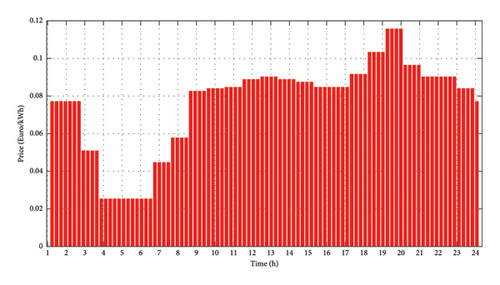
Moreover, by noticing different electricity price scenarios, as depicted in Figure 8, we can capture the stochastic behavior of the grid. The variation in electricity prices adds an important element of uncertainty and randomness to the overall grid behavior.
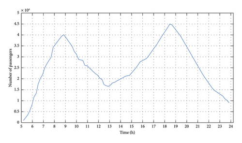
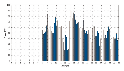
To acquire more relative results to real case, we also take into account the dynamic changes in passenger numbers (Figure 9) at the considered station. The fluctuating number of passengers indirectly impacts the amount of RBE generated by causing variations in the total mass of the train (Figure 10), which in that way stochastic behavior of the RBE will be satisfied. In this context, RBE is assumed as energy that is indirectly supplied to the grid through the ESS.
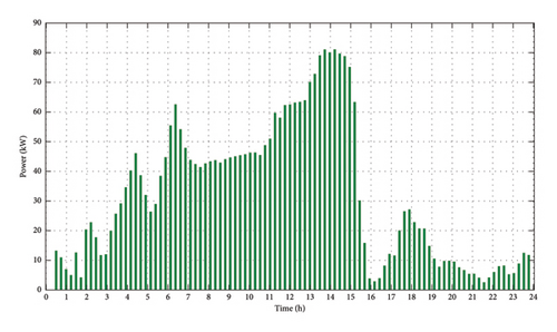
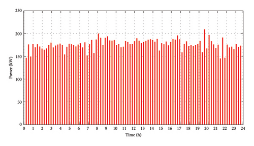
In this study, the station load demand is a crucial factor that has been thoroughly examined and is illustrated in Figure 11. As mentioned before, it encompasses several significant components such as elevators, escalators, lighting, passengers’ information systems, heating, air conditioning, and commercial users.
Drawing insights from our prior research, particularly in [5], the experiences and outcomes from that study provide valuable considerations for understanding the applicability of the modern methods in the specific context of energy management. It is noteworthy that Table 3 serves as a valuable tool for a comprehensive overview of modern methods, facilitating a clearer understanding of their comparative performance in the context of energy management. While the table offers a general performance comparison, it is crucial to recognize that the suitability and efficacy of each method can vary significantly based on the specific nuances of the energy management problem at hand. Factors such as data availability, system constraints, objectives, and modeling assumptions all contribute to this variability. A thorough assessment of these considerations is indispensable for identifying the most fitting optimization technique tailored to the unique needs of your EMS.
| Technique | Speed | Simplicity | Efficiency | Robustness | Accuracy | Performance |
|---|---|---|---|---|---|---|
| NLP | Varies based on problem complexity and solver efficiency | Moderate complexity due to nonlinear nature | Can handle large-scale problems efficiently with suitable solvers | Sensitive to problem formulation and initial conditions | Highly dependent on problem formulation and solution approach | Can provide high-quality solutions, but convergence may not always be guaranteed |
| DEA | Fast and efficient | Relatively simple | Can handle large datasets efficiently | Robust against outliers and noise in the data | Based on relative efficiency rather than absolute accuracy | Provides comparative efficiency scores and rankings |
| MCS | Moderate speed | Relatively simple | Computationally demanding for a large number of iterations | Robust in capturing uncertainty and variability | Accuracy depends on the quality of probability distributions used | Provides probabilistic outputs and risk analysis results |
| MILP | Varies based on problem complexity and solver efficiency | Moderate complexity due to integer variables | Can handle large-scale problems with efficient solvers | Robust against problem formulation and constraints | High accuracy in finding optimal or near-optimal solutions | Provides optimal solutions and guarantees optimality under certain conditions |
In the broader landscape, contemporary methods such as DE, dynamic programming (DP), Monte Carlo simulation (MCS), MILP, and NLP showcase advanced capabilities in handling intricate and nonlinear optimization challenges within railway EMSs. These methods offer heightened flexibility, superior global optimization guarantees, and adeptness in managing discrete variables or dynamic scenarios. However, the optimal choice among these methods hinges on factors such as problem characteristics, computational resources, and the delicate balance between solution quality and computational efficiency. And based on high efficiency, robustness, accuracy, and performance of MILP, we chose this method for our work.
In REMS, the integration of various cutting-edge technologies lies at the core of achieving concurrent utilization of different energy types. First, we implement hybrid energy systems, strategically combining the attributes of multiple sources such as wind and solar energy. By strategically situating WTs and solar panels to complement each other’s generation patterns, a harmonized and uninterrupted power supply is ensured.
Second, the pivotal role of ESS comes into play within this integrated framework. Advanced batteries and super capacitors are employed to capture excess energy during peak periods, releasing it during low-production phases. This dynamic process effectively mitigates the intermittent nature of renewable sources, contributing to a stable and continuous energy output.
Furthermore, the implementation of smart grid architecture is crucial for seamless coordination and control of diverse energy inputs. Smart grids actively manage energy distribution, optimizing the utilization of different sources based on real-time demand and availability. Additionally, strategically integrated power converters play a vital role, converting energy from various sources into a standardized form for efficient distribution.
The synergy of these elements, coupled with the application of MILP models for optimization, ensures a reliable, sustainable, and simultaneous utilization of different energy sources in the railway station EMS. This comprehensive approach not only enhances efficiency but also underscores the system’s adaptability and resilience in harnessing diverse energy resources.
3. Results and Discussion
- 1.
ESS scenarios (9 variations): We thoroughly explored different initial SOE for the ESS. This allowed us to investigate a wide spectrum of potential ESS setups.
- 2.
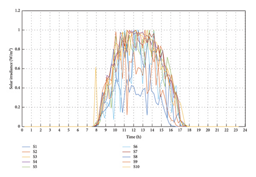
PV generation scenarios (10 variations): To capture the diverse nature of solar energy, we meticulously assessed PV generation under two distinct weather conditions: sunny and cloudy. This involved analyzing variations in solar irradiance and its consequent impact on PV output.
- 3.
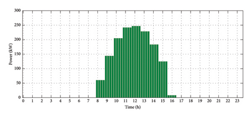
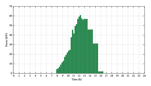
WT generation scenario (3 variations): Considering the significant role of wind power, we integrated a scenario that precisely depicted the WT generation based on the prevailing wind speeds. This offered valuable insights into the output potential of WTs.
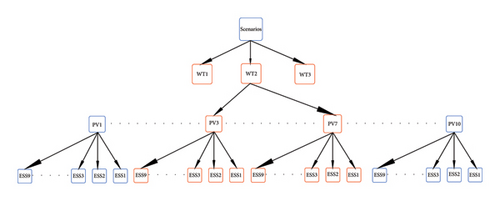
The amalgamation of these three elements yielded the exhaustive range of 36 distinct scenarios, as visually depicted in Figure 12. Each scenario represents a unique combination of ESS configuration, PV generation condition, and WT generation condition.
The results of the analysis are presented in Table 4, showcasing optimal scenarios and their corresponding outcomes. The base case, which does not include any PV panels, WT, or ESS, serves as a reference point for comparison. In Case 2, only the ESS is utilized, while Case 3 focuses solely on PV in a cloudy scenario. In Case 4, PV is examined in a sunny scenario. Case 5 incorporates both ESS and PV in a cloudy scenario, while Case 6 considers ESS and PV in a sunny scenario. Case 7 explores the combined impact of ESS, WT, and PV in a cloudy scenario, and Case 8 investigates ESS, WT, and PV in a sunny scenario. The table provides a comprehensive overview of the results, allowing for a thorough analysis of each case study and its corresponding cost reduction.
| Rows | Case description | Operational cost (€) | Reduction cost (%) |
|---|---|---|---|
| Case 1 | None of ESSs, PV, WT | 316.25 | Base case |
| Case 2 | ESSs | 306.10 | 3.2 |
| Case 3 | PV (cloudy scenario) | 274.98 | 13.04 |
| Case 4 | PV (sunny scenario) | 255.43 | 19.23 |
| Case 5 | ESSs, PV (cloudy scenario) | 223.56 | 29.3 |
| Case 6 | ESSs, PV (sunny scenario) | 204.01 | 35.49 |
| Case 7 | ESSs, PV (cloudy scenario), WT | 158.39 | 49.91 |
| Case 8 | ESSs, PV (sunny scenario), WT | 138.85 | 56.09 |
Table 4 summarizes the base case and seven optimal cases evaluated in this research, assuming different pricing schemes. The table reveals that utilizing only ESS, PV systems, or combinations of ESS, PV, and WT has a magnificent impact on reducing the total daily operational costs of the smart railway station using the stochastic approach.
In the base case, which assumes no utilization of ESS, PV, or WT, the worst-case scenario is evaluated based on the pricing signal. However, the study demonstrates that even with only ESS installed, using the REMS results in a cost reduction of 3.2% for the stochastic approach.
Moreover, the most efficient option is found to be the reuse of RBE by ESS, PV, and WT. This option achieves a 56.09% reduction in costs for the stochastic approach.
The findings highlight the significant benefits of incorporating ESS, PV, and WT in reducing the operational costs of smart railway stations. Implementing REMS and utilizing RBE alongside ESSs and RERs further enhance cost savings, making them highly advantageous options.
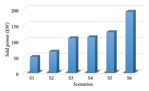
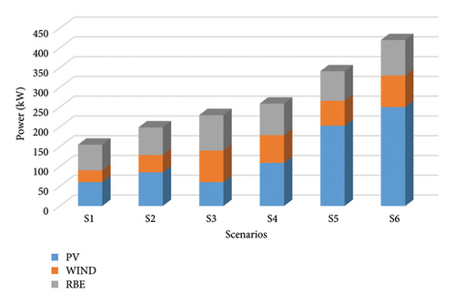
The implementation of the smart grid architecture in this study has established a bidirectional power flow at the smart railway station. This foundation enables the seamless integration of RERs. Figure 13 depicts the power sold back to the grid in convenient 24 h intervals for 6 scenarios. Notably, the stability of the sold power varies based on different scenarios, such as a combination of WT and a PV generation—sunny day, as opposed to a cloudy one. Also, Figure 14 showcases the decomposition of generated power, focusing on the contributions of PV panels, WTs, and RBE, to sell to the grid across these six different scenarios.
4. Conclusions
Researchers have proposed several approaches to address the increasing greenhouse gas emissions and CO2 emissions in the railway industry, as well as the energy shortage. This study introduces a REMS that incorporates RERs and ESSs and utilizes RBE. The stochastic behavior of PV panels, influenced by varying solar irradiation levels, and different wind speeds affecting the WT, along with various initial SOE levels of ESSs, passenger numbers throughout the day, and pricing signals from the main grid, are considered.
This study implements a MILP model to minimize the total daily operational cost of a smart railway station. Also, probabilistic behavior is incorporated to account for the likelihood of different solar irradiation levels and wind speeds occurring. To simplify the analysis, 36 different scenarios are selected. Following the base case definition, Case 2 demonstrates a 3.2% cost reduction by utilizing ESSs. The implementation of PV panels in two scenarios (cloudy and sunny) results in cost reductions of 13.04% and 19.23%, respectively. Furthermore, combining ESSs with PV panels in two scenarios (cloudy and sunny) reduced operational costs by 29.3% and 35.49%, respectively.
In Cases 7 and 8, the addition of a WT to the previous cases led to significant cost reductions of 49.91% and 56.09%, respectively. Additionally, through the implementation of smart grid architecture and bidirectional power flow between the grid and the station, the most effective scenario enables the sale of 190.8 kW of power to the grid in a single day.
The authors underscore the forward-looking potential of this research, envisioning a future where the REMS seamlessly converges with EV smart parking lots. This innovative integration promises to create a holistic and sustainable urban mobility ecosystem, optimizing energy usage not only within railway stations but also in the burgeoning realm of electric transportation. Furthermore, the authors advocate for the incorporation of machine learning methodologies to elevate the REMS to new heights of sophistication. Envisioned enhancements include predictive energy consumption modeling, anomaly detection, fault diagnosis, and the implementation of optimal energy allocation strategies. The integration of adaptive control strategies further fortifies the system’s resilience and responsiveness. These transformative synergies between REMS, EV infrastructure, and machine learning present an exciting and multifaceted avenue for future research and exploration, promising groundbreaking contributions to the realms of energy efficiency, transportation sustainability, and smart urban development.
Disclosure
This manuscript reflects only the authors’ views and opinions; neither the European Union nor the European Commission can be considered responsible for them.
Conflicts of Interest
The authors declare no conflicts of interest.
Funding
This study was carried out within the MOST—Sustainable Mobility National Research Center and received funding from the European Union Next-Generation EU (PIANO NAZIONALE DI RIPRESA E RESILIENZA (PNRR)—MISSIONE 4 COMPONENTE 2, INVESTIMENTO 1.4—D.D. 1033 17/06/2022, CN00000023).
Open Research
Data Availability Statement
Due to the institutional data usage limitations and privacy policies, the data supporting the findings of this study are not publicly available.


