This paper proposes a multiagent reinforcement learning (MARL) approach to optimize energy management in a grid-connected microgrid (MG). Renewable energy resources (RES) and customers are modeled as autonomous agents using reinforcement learning (RL) to interact with their environment. Agents are unaware of the actions or presence of others, which ensures privacy. Each agent aims to maximize its expected rewards individually. A double auction (DA) algorithm determines the price of the internal market. After market clearing, any unmet loads or excess energy are exchanged with the main grid. The New Energy Lab (NEL) at Staffordshire University is used as a case study, including wind turbines (WTs), photovoltaic (PV) panels, a fuel cell (FC), a battery, and various loads. We introduce a model-free Q-learning (QL) algorithm for managing energy in the NEL. Agents explore the environment, evaluate state-action pairs, and operate in a decentralized manner during training and implementation. The algorithm selects actions that maximize long-term value. To fairly consider the algorithms for both customers and producers, a fairness factor criterion is used. QL achieves a fairness factor of 1.2643, compared to 1.2358 for MC. It also has a shorter training time of 1483 compared with 1879.74 for MC and requires less memory, making it more efficient.

1. Introduction

The electric power industry is facing numerous challenges, including depleting fossil fuel resources, regulatory and public pressure to cut pollution, growing energy demand, and aging infrastructure. Despite these difficulties, the industry has access to abundant clean energy resources, such as solar and wind power, which offer promising solutions [1]. In the future net zero buildings, natural gas, as an energy carrier, will need to be replaced by renewable energy systems including, photovoltaic (PV) panels, small wind turbines (WTs), renewable hydrogen, H2 fuel cell (FC), and energy storage systems (e.g., battery, H2 generation, and storage). Microgrids (MGs) are becoming increasingly important in today’s power systems because they enhance reliability, integrate renewable energy sources (RESs), improve energy efficiency, reduce costs, and increase energy availability [2]. According to the International Council on Large Electric Systems (CIGRE), MGs are defined as electricity distribution systems containing loads and distributed energy resources (DERs). These systems can operate in a controlled and coordinated manner, whether connected to the main grid or functioning independently in the islanded mode [3]. However, integrating DERs poses significant challenges for maintaining the stable and economical operation of a MG. The intermittent and stochastic nature of DERs, such as PV and WT, introduces uncertainty in energy generation. Combined with load variations, these uncertainties make it difficult to develop accurate generation schedules [4]. An energy management system (EMS) is a systematic approach to optimizing, planning, controlling, monitoring, and conserving energy. Its goal is to enhance operational efficiency and reduce energy consumption [5]. Numerous articles are devoted to managing energy in MGs. The authors in [6] used mixed integer linear programming to minimize fuel costs, employing a piecewise linear function for diesel generators. Notably, their work does not account for the uncertainties associated with PV generation and load demand. In [7], the authors present a modified particle swarm optimization algorithm for real-time energy management in grid-connected MGs, achieving a significant reduction in operational costs. The authors in [8] utilized the multiobjective nondominated sorting genetic algorithm II. This approach is aimed at optimizing energy management in MGs, with a primary focus on reducing costs and environmental pollution. In [9], the article focuses on the application of model predictive control (MPC) for energy management in grid-connected smart buildings with electric vehicles (EVs). The MPC-based EMS involves forecasting information on building demand and EV charging demand to optimize energy consumption and cost. The study assesses the effectiveness of MPC in achieving efficient energy management in the context of grid-connected smart buildings with EVs. In [10], the authors implemented an advanced EMS in a community of buildings by using nonlinear MPC based on successive linear programming. They optimized electricity flow by considering real-time factors such as weather forecasts and market prices. All the previously mentioned methods for managing energy in MGs rely on utilizing the system’s model estimation. Creating a model-based energy management strategy for a MG necessitates expertise in modeling each system component. The choice of models and parameters can significantly impact the results or predictions, and it is important to carefully consider and validate these selections to ensure the robustness and generalizability of the models. Inaccurate probability distribution models, coupled with low-accuracy parameters, hinder traditional model-based methods, leading to suboptimal solutions. In addition, adapting to changes in MG topology, scale, or capacity requires system remodeling and solver redesign, a process that is both cumbersome and time-consuming [11]. This typically occurs due to the complexity of the environment, making the priori design of effective agent behaviors challenging or even impossible. In addition, in a dynamic environment, a preprogrammed behavior may become unsuitable over time [12]. As an alternative to model-based approaches, learning-based algorithms have surfaced in recent years. They hold the potential to reduce dependence on explicit system models, improve the scalability of EMS, and decrease associated maintenance costs [13]. In recent years, there has been growing enthusiasm among academic and industrial research for energy management methods based on machine learning and artificial intelligence [14]. Reinforcement learning (RL) is one branch of machine learning that has been extensively applied to perform complex tasks, spanning from games [15] to robotics [16]. Lots of work has been devoted to using RL in managing energy in smart grids. For instance, in [17], a decentralized Q-learning (QL) algorithm was utilized to manage energy in a MG containing various energy resources. The performance of the agents was compared under four scenarios, which include no learning, generator learning, customer learning, and whole learning. In [18], the authors presented a novel decentralized multiagent approach for energy management in a grid-connected MG, incorporating both electrical and thermal power. Their approach treated energy generators and consumers as autonomous agents capable of making decisions, each seeking to maximize their own profit using a model-free QL algorithm. The study evaluated three different action selection methods and compared their results. This approach holds promise for more efficient and effective energy management in MG systems. In [19], a multiagent-based model is used to study energy management in a MG. In this article, WT, PV panel, diesel generator, and battery were considered within the MG. QL was used to solve the energy management problem. Loads were considered as active agents, which can curtail their demand in order to achieve more profit. The main focus of [20] has been on mitigating fluctuations and mismatches between power supply and demand. To tackle this issue, they introduced an innovative approach known as the enhanced RL-based method. By using the SARSA algorithm in RL, this method mainly optimizes energy usage from renewable sources like solar panels. The main objective of their work is to maximize the utilization of renewable energy while minimizing the consumption of fossil fuel energy. In [21], a novel SARSA-based method was proposed to solve a complex scenario-based nonconvex optimization problem. In [22], a method for managing energy in a multi-MG environment is introduced. To determine the retail price, the MC method was employed. It enhances decision-making by using predictive techniques, aiming to maximize profits from power sales while minimizing the peak-to-average ratio. The authors in [23] utilized the MC method to handle uncertainties in wind power, aiming to generate profits from wind energy investments. Numerous studies have delved into the domain of energy management in MGs. The distributed architecture of these agents allows for the application of this optimization technique as a decentralized control strategy employed in MG EMS [24]. The significant research gap in the literature is that none of the referenced articles integrate practical settings into their research methodologies. Consequently, there is a lack of comprehensive research aimed at validating theoretical concepts in real-world scenarios and utilizing real technical data. Hence, this article develops a smart and efficient scheduling mechanism for optimizing the performance of a MAS-based EMS in a practical setting to address real-world challenges. Therefore, the New Energy Lab (NEL) training set [25] is selected, a facility equipped with different DERs and some loads. Notably, this lab can be seamlessly integrated with the power main grid. A fully decentralized QL algorithm is proposed for the NEL’s energy management. To evaluate the performance of the presented algorithm, the simulations are conducted using real weather data. In addition, the results of the presented method are compared with SARSA and MC algorithms. Based on the simulation results, the efficiency and superiority of the proposed method are confirmed.

The primary contributions of this article can be summarized as follows:

•
A comprehensive MG model is created to simulate the components of the NEL. The model encompasses WTs, PV panels, an FC, a battery, and various loads. Each component is carefully modeled to ensure an accurate representation in the simulation.
•
The control problem is formulated as a Markov game, considering a wide range of control actions like the price of energy for all of the agents, as well as the current of the FC and battery.
•
This proposed model takes into consideration the technical constraints of DERs, as well as consumption by customer agents.
•
The market clearing process is facilitated using a DA algorithm.
•
The proposed decentralized approach is implemented using real-world data and compared with SARSA and the MC algorithm.

The remainder of this paper is organized as follows: In Section 2, we provide the model of the components of the NEL. Section 3 discusses the energy management design based on reinforcement learning, starting with the Markov game framework and its state, action, and reward components in the multiagent NEL environment. It then covers QL, SARSA, and Monte Carlo algorithms, followed by hyperparameter tuning and the double auction algorithm. Section 4 presents the simulation results and analysis. Finally, we conclude this paper in Section 5.

2. Modeling Agents and Environment in the NEL

The NEL comprises PV panels, WTs, an FC, a battery, and various loads. It serves as an energy management platform for integrating renewable wind and solar generation with battery storage, H₂ generation through electrolysis, H₂ storage, and power regeneration using an FC. Its flexible energy management unit allows quick modifications to the system’s setup, enabling the integration of multiple renewable inputs with various energy storage options.

In this study, the NEL is approached as a multiagent system (MAS), where each DER, battery, and load is modeled as an autonomous agent. An agent is an entity capable of perceiving its environment, processing information, and taking actions to achieve specific objectives. These agents operate in a fully decentralized manner, making independent decisions based on local observations while interacting through a shared communication network.

At the system level, the MAS ensures efficient resource utilization, minimizes reliance on the main grid, and guarantees reliable energy balancing. The scalable decentralized framework allows the seamless integration of additional agents without disrupting the learning process, while maintaining flexibility to adapt to dynamic changes in system configuration and operational goals.

The architecture of the NEL system is depicted in Figure 1, providing a visual representation of its components and interactions.

Details are in the caption following the image — **Figure 1**
Open in figure viewer PowerPoint

Visualization of the NEL system [25].

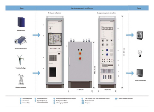
The NEL is connected to the main grid via a bidirectional power flow and a communication channel.

In the following, mathematical models of different agents are given.

2.1. WT

The output power from WT is a function of wind speed v(t) and can be derived using the following equation [26–28]:

()

where P and P_r indicate the output power and rated power of WT, respectively. v_r, v_ci, and v_co represent the rated wind speed, cut-in speed, and cut-out speed, respectively.

2.2. PV Panels

The output power of the PV module at solar irradiance s (watt/m²) and temperature T in °C can be expressed as follows [29]:

()

where

()

In the context of this equation, T and T_A correspond to the cell and ambient temperatures, expressed in °C. K_i and K_v denote the current and voltage temperature coefficients, measured in amperes/°C and volts/°C, respectively. N_OT signifies the nominal operating temperature of the cell in °C, and V_oc and I_sc stand for the open circuit voltage and short circuit current. V_M and I_M, respectively, refer to the voltage and current at the maximum power point.

2.3. FC

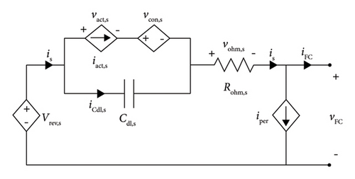
Figure 2 illustrates the model depicting the electrical performance of the FC in both steady-state and dynamic operational modes [30].

2.3.1. Thermodynamic Phenomena

By applying thermodynamic laws to this reaction and utilizing the Nernst equation, the reversible voltage of the cell is obtained as follows:

()

The cell operating temperature is represented by T in °C, while and correspond to the hydrogen and oxygen pressures, respectively, measured in bars.

The following equation is proposed to establish a relationship between the

with the i_FC:

()

2.3.2. Activation Phenomena

The overvoltage caused by this phenomenon is known as activation voltage.

In order to experimentally obtain v_act, one can use the following equations:

()

where a and b are parameters that depend on the cell temperature in °C, as follows:

()

2.3.3. Concentration Phenomena

The cell concentration overvoltage v_con is related to the concentration current i_con and can be obtained through the following empirical equation:

()

where we have

()

2.3.4. Double Layer Phenomena

Given the fact that the FC has N_s series connected cells, the FC double layer capacitor C_dl,s is obtained from the FC double layer capacitor C_dl through the following equation:

()

2.3.5. Ohmic Phenomena

v_ohm(t) can be generically represented based on Ohm’s law as follows:

()

where we have

()

2.3.6. Peripheral Energy Consumption

The equation for the current source modeling the FC peripherals and which relates the FC current i_FC(t) and the peripherals current i_per(t) is as follows:

()

2.4. Battery

In [31], the Manegon model of the battery is given, and it has two modes: discharge mode and charge mode.

2.4.1. Discharge Mode

The discharge voltage is given by the following equation:

()

where T represents the internal battery temperature in °C, T_a denotes the ambient temperature in °C, and C stands for the battery nominal capacity in Ah, and SoC(t) shows the state of charge (SoC) of the battery at time t.

During the discharge mode, a linear decrease in SoC occurs as the utility is supplied by the battery over time.

()

where SoC₀(t) represents the initial value of the SoC at time t and Δt is the time interval, measured in hours.

2.4.2. Charge Mode

The output voltage evolution and SoC(t) during the charging mode are provided in the following:

()

2.5. Loads

In this article, we categorize loads into two types: critical appliances and curtailable appliances.

•
Critical appliances, such as refrigerators, are essential for daily life and must always receive their full power demand. Since these appliances cannot be turned off or reduced without causing inconvenience or disruption, they are excluded from the demand response program.
•
Curtailable appliances, such as air conditioners and water heaters, offer more flexibility. Their power consumption can be adjusted based on system conditions, electricity prices, or incentives, making them valuable participants in the DR program.

Each load acts as an independent agent, deciding how much energy it can reduce when needed. This flexibility helps balance supply and demand, reduce peak loads, and lower electricity costs. By allowing real-time adjustments, curtailable loads also make it easier to integrate renewable energy sources into the microgrid, leading to a more stable and efficient energy system.

2.6. Environment Design

Due to the intermittent and uncontrollable nature of DERs, they cannot meet the entire demand independently. As a solution, the NEL is connected to the main grid, serving as an additional reserve. Initially, producers and consumers specify their energy supply and demand. After the DA agent clears the price, surplus energy from producers is sold to the main grid, and consumers buy their unsatisfied energy from it. For these transactions, the main grid determines its buying and selling prices at each time step, denoted as Pr_B (t) and Pr_S (t), respectively. It is imperative to ensure that the generation dispatch at each time step should meet the following power balance constraint:

()

P_WT(t), P_pv(t), and P_fuel(t) denote the energy generation from WT, PV panel, and FC at time t, respectively. P_battery(t) shows the power of battery at time t, and its sign depends on whether it is acting as a buyer or a seller. When functioning as a buyer, it has a positive sign; otherwise, it has a negative value. The values d₁(t)–d₅(t) represent the load demand of customers one to five at time t, respectively.

represents the power purchased from the main grid and

represents the power sold to the main grid at time slot t. To maintain balance, the following constraints must be satisfied:

()

where

is the maximum transaction power limit between main grid and MG at time slot t.

The profit of main grid can be written by the following formula [4].

()

3. Energy Management Design Based on RL

In MGs, agents’ profit depends on their own actions and the actions of other agents. Due to the stochastic nature of the MG environments, agents do not follow predetermined and fixed policies; they continuously adapt their strategies to maximize their profits. To represent these dynamic and nonstationary interactions among agents within MGs, the Markov game framework is suitable. Markov games are extensions of MDPs to MASs, in which multiple actions are chosen and executed at the same time, resulting in new states that are influenced by the actions taken by each individual agent [32].

A Markov game is a tuple , in which N shows the number of agents, S is a finite set of states, A is the action set where each A_i is the action set of agents i ϵ N, P is the transition probability which indicates the probability of going to new state given the current states and actions, R_i is the reward function of agent i, and γϵ(0, 1] is the discount factor [33].

3.1. Design of Agents’ Elements in Markov Game

In the Markov game setting, producer agents aim to maximize their profits, while customers seek to minimize costs. The primary objective is to reduce reliance on the main grid by establishing a self-sufficient MG. A summary of the agent’s role, state, action, immediate reward, and objective of all agents is provided in Table 1.

Table 1. State, action, and reward representation of all agents in the NEL multiagent environment.

Agent’s name	Agent’s role	States	Actions	Immediate rewards	Objectives
WT	Energy producer	(t, PrS, PrB)	Price of WT energy	profit_WT − cost_WT	Maximize profit of selling produced energy

PV	Energy producer	(t, PrS, PrB)	Price of PV energy	profit_PV − cost_PV	Maximize profit of selling produced energy

FC	Energy producer	(t, PrS, PrB)	Price of FC energy, current of FC	profit_FC − cost_FC	Maximize profit of selling produced energy

Load	Energy consumer	(t, PrS, PrB)	Price of load demand, load curtailment percentage	reward_load = −(pc∗(c_i(t) + r_i(t)) + K∗\|d_i(t) − e_i(t)\|)	Minimize costs and enhance customer satisfaction

Battery	Energy storage	(t, PrS, PrB, SoC)	Price of battery energy, current of battery	• If battery is seller and PrS = >40reward_Battery = ((Profit_Battery)/(totalp))∗100 + 8 • If battery is seller and PrS < 40reward_Battery = ((profit_Battery)/(totalp))∗100 − 200 • If current_Battery = 0reward_Battery = 16 • If battery is buyer and PrS > 16reward_Battery = (1 + (profit_Battery)/(totalp))∗50 − 200 • If battery is buyer and PrS < = 16reward_Battery = (1 + (profit_Battery/totalp))∗50 + 30 totalp = 0.45	Optimize charge/discharge cycles

Next, we describe the key elements of the Markov game, including states, actions, and rewards.

3.1.1. Description of State Elements in the NEL Multiagent Environment

Selecting an appropriate state space is crucial for each agent, as it should provide relevant information for decision-making while avoiding redundancy. In the NEL multiagent environment, we have outlined the relevant states for each agent in Table 1. In the following, we provide a detailed description of the components of these states and how each element supports the specific objectives of the agents.

•
The time of day serves as a valuable indicator for all agents, as demand fluctuations, renewable energy availability, and grid congestion can depend on the time. This helps in identifying patterns more effectively.
•
The prices for buying and selling energy from the main grid are chosen as states for all agents, providing essential information on the current energy cost. This enables both producers and consumers to make informed decisions about their energy bids. Producers, for example, can choose to sell energy to the grid when prices are high, thereby maximizing their revenue, while consumers can decide whether to purchase energy from the main grid based on the affordability of the prices. By relying on real-time price data, both types of agents can improve their operations and contribute to more efficient energy management.
•
The SoC of the battery is selected as a state for the battery agent to represent available energy storage capacity. This enables strategic management of battery usage, balancing supply and demand, reducing reliance on the main grid, and addressing the intermittency of renewable energy sources.

3.1.2. Description of Action Elements in the NEL Multiagent Environment

Actions play a crucial role in RL, as they determine the decisions made by an agent, directly influencing its future states and rewards, thereby guiding its learning process. In the NEL multiagent environment, we have carefully defined the corresponding actions for each agent, as outlined in Table 1. In the following section, we will provide an in-depth description of the elements that make up these actions, highlighting how each element is designed to facilitate the specific objectives of each agent.

•
PV and WT, as nondispatchable energy sources, generate power based on environmental factors such as solar irradiance, temperature, and wind speed. Due to their dependence on these fluctuating variables, their energy output is inherently variable and cannot be controlled to match demand. As such, no action is defined for controlling their energy output. In contrast, FCs are dispatchable, as their energy output can be adjusted by controlling the operating current, which is chosen as an action to allow regulation in response to demand.
•
Batteries enhance energy management by optimizing energy storage, meeting demand requirements, and contributing to grid stability. This is achieved through the precise control of charge and discharge currents, with battery current specifically chosen as an action for regulating their energy output.
•
All producer agents, batteries, and loads determine the prices for their energy production and consumption, enabling producers to strategically set prices for revenue optimization and consumers to minimize costs, while taking into account factors such as demand, supply, and market conditions.
•
Customers’ action is the percentage of their load they choose to curtail, representing their willingness to reduce electricity consumption. They select a curtailment percentage from the set {0, 0.05, …, 0.65, 0.70}. A selection of 0 means the customer opts not to curtail any part of their load, maintaining full electricity usage. Conversely, a selection of 0.7 indicates that the customer curtails 70% of their load, significantly lowering their electricity consumption to contribute to system efficiency or cost savings.

3.1.3. Description of Reward Elements in the NEL Multiagent Environment

In the NEL multiagent environment, a specific reward is defined for each agent based on its actions and performance, supporting decentralized decision-making. This allows each agent to independently optimize its behavior according to its unique goals, enhancing flexibility and efficiency. The approach also promotes scalability and robustness, as agents can adapt to local conditions without relying on centralized control. In the following section, we will provide a detailed explanation of the reward elements, emphasizing how each is tailored to support the specific objectives of each agent.

•
The rewards for producers, such as PV, WT, and FCs, are defined based on the profit they earn from selling their generated energy, either directly to local loads or to the main grid. These rewards are higher when they sell energy within the internal market, which offers greater profits compared with selling excess energy to the grid. The main grid encourages this behavior by prioritizing the utilization of green energy, reinforcing the incentive with a lower purchase price for energy bought by the grid.
()
•
The reward for the customers balances cost and satisfaction. In each time slot t, every customer i has an accumulated load demand, denoted as d_i(t), which represents the total energy they wish to consume for their appliances within that time slot. The desired energy consumption of customer i for their critical load and curtailable load at time slot t is represented by c_i(t) and r_i(t), respectively. Thus, d_i(t) can be expressed as d_i(t) = c_i(t) + r_i(t). After customer i consumes energy e_i(t) during time-slot t, it fulfills a portion of d_i(t), and the remainder, denoted as d_i(t) − e_i(t), remains unsatisfied. This unsatisfied load demand, referred to as the remaining load demand, leads to customer dissatisfaction during that time slot. Besides the price of energy that customer agent must pay, we have the penalized part, the unsatisfied amount of load will appear in the cost function. The reward of the customer’s energy at each time step is written as follows [19].
()
The value of K can be selected based on customer preferences. For instance, customers who prioritize having all their appliances fully satisfied need to choose a higher K. The system adjusts dynamically to these preferences, ensuring that rewards are optimized to effectively align with individual priorities. In this formula, pc shows the mean of energy price in the main grid.
•
The battery operates in three distinct modes: charging, discharging, and idle. Each mode has a specific reward mechanism designed to guide the battery’s behavior and ensure efficient energy management.
- 1.
  Charging mode (battery as a buyer)
- In the charging mode, the battery stores energy for future use. The reward formula is
  ()
- The parameter a plays a crucial role in encouraging or discouraging charging based on the selling price of energy by the main grid. We consider two following scenarios.
- First, high selling price (PrS〉P₁): a negative value is assigned to a, discouraging charging during high selling prices. This ensures the battery does not store energy when it is more profitable to sell.
- Second, low selling price (PrS ≤ P₁): a positive value is assigned to a, encouraging the battery to charge when energy prices are low, maximizing cost-effectiveness.
- 2.
  Discharging mode (battery as a seller)
- In the discharging mode, the battery releases stored energy to the grid or consumers. The reward formula is
  ()
- The parameter b determines the reward based on the selling price.
- First, high selling price (PrS ≥ P₂): a positive value is assigned to b, encouraging the battery to discharge during periods of high profitability.
- Second, low selling price (PrS < P₂): a negative value is assigned to b, penalizing discharging during low selling prices to avoid financial loss.
- 3.
  Idle mode (no energy exchange)
- When the battery is idle, it neither charges nor discharges. The reward is fixed as follows:
  ()
- The idle mode plays a crucial role in enhancing the overall efficiency and reliability of the system. By avoiding energy exchanges under unfavorable conditions, it enables more informed decision-making, ensuring that the battery is utilized only when it yields maximum benefits. This approach not only optimizes resource allocation but also enhances the system’s economic efficiency by preventing energy losses associated with inefficient charging and discharging. Furthermore, the idle mode significantly improves battery longevity by minimizing excessive cycling, thereby reducing capacity degradation over time. As a result, this mode supports both operational sustainability and long-term system stability, establishing it as a key element of energy management strategies.

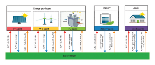
Figure 3 provides a visual representation of the NEL environment, highlighting the states, actions, and rewards associated with each agent in the multiagent setup. In this decentralized framework, agents operate independently, without awareness of each other’s existence, and interact solely with the environment to make decisions.

3.1.3.1. Cumulative Reward: System-Wide Performance

The cumulative reward represents the total reward of all agents in the system, including producers (WT, PV, and FC) and consumers (loads). It provides a unified measure of system performance by summing the individual rewards of all agents:

()

A higher cumulative reward indicates better overall coordination and efficiency among agents, reflecting an improved multiagent energy management strategy.

3.2. Multiagent Reinforcement Learning (MARL) Algorithms: An Overview of QL, SARSA, and Monte Carlo

RL is utilized for managing energy in MGs due to its capability to dynamically optimize energy distribution, storage, and consumption, adapt to changing conditions, handle complex decision-making tasks, provide flexibility in exploring strategies, and improve efficiency and reliability.

In RL, achieving an effective balance between exploration and exploitation is essential for agent success. Exploration involves trying new actions to discover potentially better strategies, while exploitation focuses on selecting the best-known actions to maximize immediate rewards. An overemphasis on exploration may delay convergence, while excessive exploitation can cause the agent to become stuck in suboptimal strategies.

In this article, the epsilon-greedy algorithm is used for choosing actions in the learning process as it effectively balances exploration and exploitation. In the ε-greedy scheme, the agent selects the action with the highest Q-value with a probability of 1 − ε or explores a random action with a probability of ε. It is beneficial for ε to vary over time; initially, it is set to a high value, promoting random action selection. As training progresses, ϵ gradually decreases, allowing the agent to shift from exploration to exploitation and better utilize accumulated knowledge [34].

The epsilon-greedy algorithm was chosen for its simplicity, flexibility, and computational efficiency, which make it suitable for real-time energy management. The algorithm’s smooth transition from exploration in early training to exploitation in later stages ensures that agents discover effective strategies while achieving stable performance.

In the following section, we will present a detailed explanation of the various algorithms employed in this article.

3.2.1. QL

This algorithm is a model-free off-policy. It means that for finding the optimal policy, the agents do not involve in constructing a model of the environment. It helps an agent to learn the optimal actions in different states by estimating their expected rewards. In RL, the learner (decision-maker) is called the agent and everything outside the agent is called the environment. The agent interacts with the environment over a sequence of discrete time steps (t = 0, 1, 2, 3, …). At each time step t, the agent receives a state, S_t ∈ S from the environment, where S is the set of possible states. Based on that state, the agent selects an action, A_t ∈ A (S_t), where A (S_t) is the set of actions available in the state S_t and it receives a reward, R_t ∈ R, and finds itself in a new state, S_t+1. The pseudocode for the QL algorithm for each agent is provided in the following (Algorithm 1).

Algorithm 1: Pseudocode of the QL algorithm for multiagent reinforcement learning.

Initialize Q (s^p, a^p) arbitrarily for all states s^p and actions a^p
For each episode:
Initialize for each agent p
Repeat for each step of the episode (t = 0, 1, 2, …, T − 1):
For each agent p:
Choose action using ε-greedy policy
Execute actions and observe reward for each agent p, and next state for each agent p
For each agent p:
Compute # Best action in next state
Update Q-value using the following formula:
Set
Until terminal condition (end of episode).

In this formula, α is the learning rate and determines in which degree the agent blends new information into its prior ones. Agents who care about their immediate reward choose a higher learning rate [33]. The discount factor γ determines the importance of future rewards [35]. Agents which think that expected future reward is much more valuable to them choose a higher discount factor.

3.2.2. SARSA

The SARSA [36] is a model free on-policy RL algorithm. A SARSA agent interacts with the environment and updates the policy based on actions taken, hence this is known as an on-policy learning algorithm. The pseudocode for the SARSA algorithm for each agent is given in the following (Algorithm 2).

Algorithm 2: Pseudocode of the SARSA algorithm for multiagent reinforcement learning.

Initialize Q (s^p, a^p) arbitrarily for all states s^p and actions a^p
For each episode:
Initialize for each agent p
Choose action using ε-greedy policy for each agent p
Repeat for each step of the episode (t = 0, 1, 2, …, T − 1):
Observe reward for each agent p, and next state for each agent p
Choose action using ε-greedy policy for each agent p
# Update Q-value using the SARSA formula:
# # Update state and action for next iteration.
Set
Until terminal condition (end of episode).

3.2.3. Monte Carlo

The Monte Carlo method also belongs to the category of model-free approaches. This method is an off-policy method. In order to acquire state and reward information, the Monte Carlo method employs a straightforward policy. It calculates the reward value by taking the average of sample rewards for a specific action. By leveraging the law of large numbers, which states that with a sufficient number of simulations and an adequate sample of rewards, the average value approximates the true value, the validity of the Monte Carlo method is confirmed [22]. The procedural form of the algorithm is shown in the following (Algorithm 3).

Algorithm 3: Pseudocode of the MC algorithm for multiagent reinforcement learning.

Initialize:
arbitrarily for all s ∈ S for each agent p
Return^p(s) ⟵ an empty list for all s ∈ S for each agent p
Loop forever (for each episode).
Generate an episode following policy
G^p⟵0 # Initialize return
Loop for each step of episode, t = T − 1, T − 2, …, 0:
Append G^p to

3.3. Hyperparameter Tunning

Hyperparameters like the discount factor and learning rate need to be tuned in RL to optimize the agent’s learning process and improve its performance. These hyperparameters influence the agent’s exploration–exploitation trade-off, convergence rate, and overall stability, impacting its ability to learn an effective policy and achieve desired outcomes in various environments. For finding the optimal value of each agent in each algorithm, the learning rate and discount factor of all the agents except the one that is examined are considered to be 0.5 and then the optimal value for the considered agent is calculated.

The parameters a, b, and c and the price thresholds P₁ and P₂, which influence the battery’s reward mechanism, are determined through an iterative trial-and-error approach. This process ensures that the reward structure effectively supports the system’s operational objectives.

3.4. Double Auction Procedure for Energy Management of the NEL

Auctions can be categorized into two types: single auctions, in which a single seller (or buyer) receives quotations from multiple buyers (or sellers), and DAs, which permit multiple buyers and sellers to bid or ask for a specified commodity [37]. The relationship between supply and demand in MGs exhibits a multibuyer and multiseller pattern. Therefore, the DA format is well-suited for MG markets. Buyers and sellers must take into account not only the quotations of other buyers (or sellers) but also the prices set by sellers (or buyers). Consequently, the decision-making process for trading strategies in a DA market is more intricate compared with a single auction [38]. In this article, we use a DA-based market structure, comprising a double auctioneer agent, buyer agents (customers), and seller agents (energy resources). It is worth noting that the battery agent at each time slot could be either buyer or seller based on the sign of its current (action of battery). During each time interval t, both seller and buyer agents submit their energy quantities along with corresponding prices. It is worth noting that the main grid is considered as a seller and specifies its price along with other producer agents and a battery when it functions as a seller agent. The double auctioneer agent facilitates market clearing by determining the price for energy transactions. At time slot t and in the kth round auction, the supplier’s produced energy and their respective offered price can be aggregated in QSupplier_k [39]:

()

In general, ns represents the number of all sellers, while

this number in round k. Note that Price_k is time-slot-dependent and remains constant across all rounds of auctions k, whereas Supplier_k varies in each round of auction. Similar to the suppliers, the buyer’s bid and their respective load demand can be aggregated in QDemand_k for time slot t and in the kth round auction.

()

As a general representation, n_b signifies the total number of buyers and specifically refers to this quantity in round k.

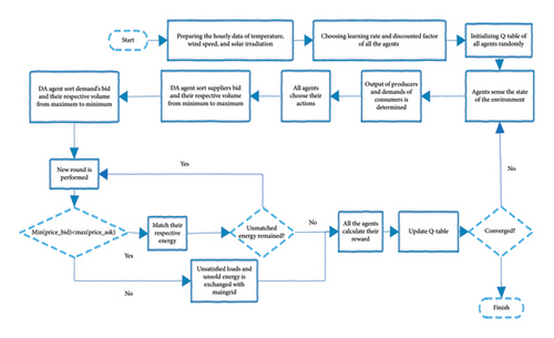
The DA agent organizes Price_k in ascending order and Bid_k in descending order. In the kth round, the minimum price is denoted as , and the maximum bid is . If , suppliers and demands will exchange their matched energy. The participating parties are the suppliers offering and the buyers bidding . If supplier i exhausts or buyer j is satisfied with , their respective quotes are removed from QSupplier_k+1 or QDemand_k+1. However, if there is still some quantity remaining for or at their specified prices, a new quote is formed, and it joins either QSupplier_k+1 or QDemand_k+1.

The auction process continues until all sellers’ or buyers’ quotes are matched or until

. We assume that there are

sellers offering

and

buyers offering

, where

≤

and

≤

. We have,

()

where

represents the energy supplied by the ith supplier and

represents the demand from the jth load, both in round k, and it is calculated by the following formula.

()

The trade volume for each seller or buyer is allocated according to their respective supply or demand proportions.

()

After the completion of the auction process, any surplus power from the sellers’ supply is sold to the main grid, while any unfulfilled demand is procured from the main grid. At time slot t, the energy supply of supplier i sold to the main grid, denoted as

, and the demand of load j purchased from the main grid, denoted as

, are described as follows:

()

In this formula, L_t represents the total number of auction round at time slot t.

In accordance with the above explanation, Figure 4 depicts the proposed algorithm for energy management within a MG based on RL.

4. Simulation and Results

In this section, we present the implementation of the proposed EMS tailored for the NEL. The simulation was executed on a laptop featuring an Intel(R) Core (TM) i7 processor and 8.00 GB of RAM. The algorithms, including QL, SARSA, and MC, were implemented using MATLAB R2020b with a decentralized control approach. Each agent independently updates its values based on local interactions with the environment, learning through exploration and exploitation within the MATLAB-defined environment.

4.1. Case Study

The simulation was carried out considering the NEL as a case study. Table 2 provides the nominal power ratings for various suppliers and loads in the NEL.

Table 2. Nominal capacity of different agents of the NEL as a case study.

Agent name	Nominal capacity (kW)	Cost of energy production (cents/kW)
PV	1	7
WT	0.4	7.8
Battery	0.4	—
Load	5 × 0.8 = 4	—

The technical parameters for the WT, PV, FC, and battery utilized in the NEL are summarized in Tables 3, 4, 5. Furthermore, the technical data employed for modeling the FC is derived from empirical results obtained for the Nexa 1200 FC, which is utilized in the NEL formulation.

Table 3. Technical data of WT of the NEL [25].

Parameter	Value
Rotor diameter	1.7 m (46 inches)
Quantity blades	3 pieces
P_r	400 W at 12.5 m/s
v_ci	3.6 m/s
v_r	12.5 m/s
v_co	49 m/s

Table 4. Technical data of photovoltaic cells of the NEL [25].

Parameter	Value
I_sc	8.63
K_i	0.055∗10⁻²
V_oc	37.4
K_v	−0.33∗10⁻²
V_M	30.7
I_M	8.15

Table 5. Technical data of lead-acid battery of the NEL [25].

Description	Value
Type	Lead-acid
Rated battery voltage	4 × 12 = 48 V
Nominal capacity C 20	55 Ah
Nominal capacity C1	34 Ah

Considering the models described in Section 2 and incorporating the weather data and technical specifications from these tables, various agents’ behaviors were simulated.

4.2. Configuration of MG

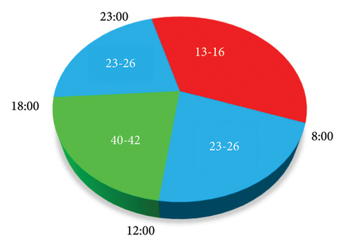
The main grid purchases electrical power from the MG at rates ranging from uniform distribution 5–15 cents per kilowatt-hour. In addition, it sells power to the MG at rates that vary, specifically at hours 23–8, 8–12, 12–18, and 18–23 from uniform distribution 13–16, 23–26, 40–42, and 23–26, respectively, as it is shown in Figure 5. To discourage the suppliers for the sole purpose of selling it to the main grid at a higher profit, the buying price of energy is set lower than the selling price.

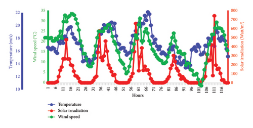
During the training and testing phases, distinct datasets are employed. The training dataset encompasses temperature, wind speed, and solar irradiation data spanning from 01/01/2018 to 01/01/2023. To augment the training dataset, additional data are generated based on the existing records. Subsequently, the testing phase utilizes data collected over 30 days, specifically from 01/07/2023 to 30/07/2023, to evaluate the effectiveness of the algorithms [40]. Figure 6 illustrates these data for five consecutive days.

As an example, Figure 7 illustrates the hourly energy outputs of WT, PV, and FC, along with the buying and selling prices of the main grid, observed over 24 h. Hourly mean profile of customers is given in Table 6 [38].

Table 6. Hourly load consumption.

Hours of a day	1	2	3	4	5	6	7	8	9	10	11	12
Load consumption (pu)	0.4	0.4	0.4	0.4	0.4	0.4	0.4	0.4	0.4	0.6	0.8	1

Hours of a day	13	14	15	16	17	18	19	20	21	22	23	24

Load consumption (pu)	1	1	1	1	1	1	1	1	1	0.8	0.6	0.5

Note: The values are per unit based on the maximum value of the load.

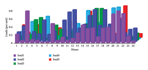
In this article, we examine five loads, each with an average of 0.8 kW. Figure 8 provides a visual representation of these loads over 24 h, which were created by using an exponential distribution. We have taken into account the following approach: 30% of each customer’s load is vital and should be fulfilled, while the remaining portion is subject to curtailment. Customers, in turn, have the ability to curtail only 70% of their load.

4.3. Sensitivity Analysis of Hyperparameters

In this article, three different algorithms are used for managing energy between generators, loads, and main grid. For all agents, we experimented with different values of epsilon in the epsilon-greedy approach, and the best result was achieved when we set epsilon to one. The optimal parameters of the agents for different algorithms are given in Table 7:

Table 7. Optimal learning rate and discount factors of different algorithms.

Agent name	QL		SARSA		MC
Agent name	Learning rate	Discount factor	Learning rate	Discount factor	Discount factor
WT	0.3	0.8	0.6	0.2	0.1
PV	0.2	0.7	0.7	0.4	0.9
FC	0.2	0.8	0.4	0.2	0.7
Battery	0.1	0.1	0.3	0.4	0.8
Load	0.4	0.9	0.9	0.3	0.2

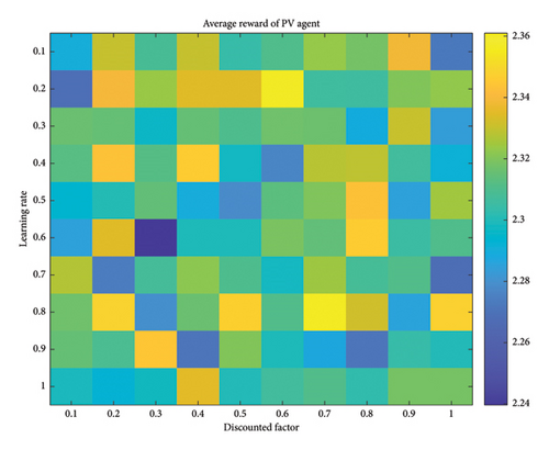
For instance, the performance of the PV agent was assessed using the QL algorithm, considering various combinations of learning rates and discount factors. Details of these evaluations are presented in Figure 9, where the profit of the PV agent is illustrated across different learning rates and discount factors. Notably, the PV agent achieves its maximum reward at a learning rate of 0.4 and a discount factor of 0.5.

4.4. Details of Markov Game Problem

Information regarding the designed state, reward, and action of these agents is provided in the following.

All of the agents select a price for the energy they intend to buy or sell value from a discrete set of prices uniformly distributed between 7 and 45 cents/kWh.

PV and WT establish the selling price of energy from the aforementioned interval. Consequently, their action space consists of nine possible values. The battery can engage in both buying and selling electricity, and they express their intention through the sign of their current. The current has one of the 5 values, including two positives, two negatives, and zero. Consequently, a battery agent’s action set comprises 9 × 5 = 45 values. Similar to the battery, an FC has the ability to select its current from the following ranges: 0, 0–10, 10–20, 20–30, 30–40, and 40–50. In summary, its action space consists of 9 × 6 = 46 values. More than choosing the price of energy for their energy demand, customers can also select their load curtailment percentage from the range {0, 0.05, …, 0.65, 0.70}. Therefore, their action space comprises 9 × 15 = 135 values.

4.5. Simulation Results and Analysis

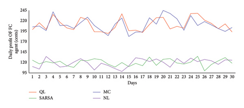
Figure 10 illustrates the daily profit of the FC agent under different algorithms. The mean profit of the MC algorithm is 211.03 cents, closely followed by the QL algorithm, which achieved a mean profit of 210.69 cents. SARSA exhibited the lowest profit among the learning algorithms at 120.06 cents, which was comparable to the NL scenario, with a mean profit of 119.61 cents. It is noteworthy that both MC and QL algorithms perform similarly, significantly outperforming the NL scenario.

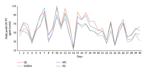
In Figure 11, the daily profits associated with various algorithms for managing the PV agent are depicted. Discerning the most effective algorithm through visual observation alone poses a challenge. According to the mean profit for the PV agent, QL demonstrates superior performance, achieving 70.24 cents. Following QL, the MC and SARSA algorithms show mean profits of 68.84 and 57.74 cents, respectively. QL and MC exhibit remarkably close performances. Surprisingly, in a scenario where agents lack learning capability, referred to as NL, the PV agent achieves a profit of 58.87 cents, even outperforming SARSA.

In Figure 12, the daily profit of the wind agent over 30 days is presented. The mean profits of the wind agent for MC, QL, and SARSA over 30 days are 107.14, 101.78, and 64.55 cents, respectively. For the NL scenario, the mean profit is 68.58 cents. It is important to highlight that both MC and QL algorithms performed well, with MC achieving the highest mean profit, followed closely by QL. However, SARSA’s performance was inferior to all of the algorithms, even NL.

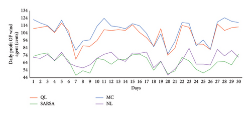
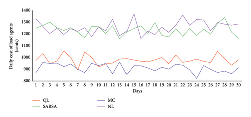
Figure 13 illustrates the daily accumulated costs of all five load agents. Notably, the cost is significantly higher when the agents lack learning capabilities. In the NL scenario, they struggle to efficiently curtail their loads and submit appropriate bids, resulting in a load cost average of 1237.89 cents in this scenario. Among the RL algorithms, MC demonstrates the best performance, with a mean cost of 910.97 cents over 30 days. Following SARSA, QL and SARSA have mean costs of 979.67 and 1234.25 cents, respectively. It is worth noting that SARSA’s performance closely mirrors the NL scenario, indicating that significant learning has not occurred in the SARSA algorithm.

One of the primary objectives for each MG is to achieve self-sufficiency and reduce reliance on the main grid, thereby minimizing transactions between the MG and the main grid. This can be accomplished by utilizing RES such as PV, WT, FC, and batteries within the NEL framework.

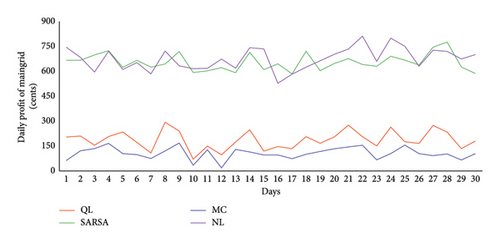
For MGs connected to the main grid, this involves reducing the financial gains of the main grid through fewer transactions. In Figure 14, the daily profit generated by different algorithms is presented. As previously discussed, an algorithm that can effectively diminish the main grid’s profit is preferable. Notably, when employing the MC algorithm across all agents, the main grid attains its lowest profit, i.e., 106.54 cents. After MC, QL and SARSA were next in performance, achieving mean profits of 185.05 and 654.86 cents, respectively. In cases where agents lack learning abilities, they tend to have the most interactions with the main grid, resulting in the highest profit for the main grid which is 675.33 cents—an undesirable outcome. It is significant to mention that the SARSA algorithm did not perform well, and its outcome closely resembles that of the NL scenario.

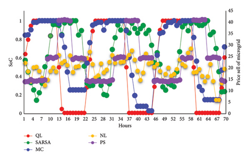
In Figure 15, the left axis displays the SoC of the battery agent under various algorithms, while the right axis shows the selling price of the main grid. It is evident that battery agent utilizing the QL algorithm effectively learn and exhibit the desired behavior as previously discussed. By using the MC algorithm, the battery agent learns to charge itself during periods of low energy prices similar to the QL algorithm. However, its performance suffers when energy prices are low, as it struggles to fully discharge itself to maximize profit. In contrast, the SARSA algorithm does not perform as well and cannot consistently follow the charge and discharge pattern seen in the QL algorithm. However, it still outperforms the NL scenario, where there is no specific pattern, and all behavior is entirely random. The mean profit of the battery in the NL scenario was −21.9 cents, and with the implementation of different learning algorithms such as SARSA, QL, and MC, it increased to −15.42, −6.06, and −6.24 cents, respectively. By using different learning algorithms, the battery’s profit remains close to zero. Several factors may contribute to this outcome. First, by the technical constraints of the NEL, the battery’s capacity is low compared with other agents, thereby hindering its ability to achieve higher profits. In addition, within MGs, the battery is primarily allocated for critical loads, such as medical facilities and emergency services, where the priority is to ensure a reliable energy supply. Furthermore, the algorithm prioritizes DER agents such as PV, WT, and FC over the battery, promoting the usage of RES in the market, and they are given precedence over the battery when all agents sell energy at the same price. However, as depicted in Figure 15, the SoC of the battery is effectively managed via QL, allowing the battery to optimize its charging and discharging based on the price of energy and thereby assisting the MG.

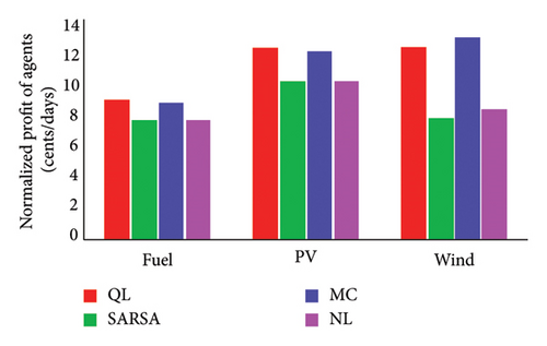
In Figure 16, the normalized profit of DER agents is depicted. We can observe that, for the FC and PV agents, the QL algorithm outperforms others, followed by the MC algorithm. In addition, the SARSA algorithm’s performance is slightly better than the NL scenario. In the case of the WT agent, the MC algorithm performs better than QL. However, for this agent, the SARSA algorithm performed worse than the NL scenario.

In summary, Table 8 presents the mean profit for various components achieved by employing different RL algorithms, while Table 9 displays the daily volume of DER agents for these algorithms. Based on the results presented in Table 8, it is apparent that MC achieves higher profits in FC, WT, and load, while QL outperforms others specifically in PV. Moreover, MC also attains the highest collective reward −523.96, followed by QL −596.96, indicating better overall system efficiency. Evaluating algorithms solely based on agent profits may not provide a comprehensive assessment. Therefore, it is imperative to establish criteria that encompass both profit and agent volume. In the next section, a criterion will be introduced to facilitate the comparison of these algorithms. This criterion will assist us in selecting the most suitable algorithm based on the preferences of all agents. As it can be seen in Table 9, the main grid volume by using learning algorithms such as QL and MC has decreased from 14.59 to −3.75 and −7.47, respectively. This shows that the dependency of the MG on main grid has reduced and in addition, the MG has sold power to main grid.

Table 8. Average of daily profit of DER agents and main grid as well as cost of loads.

Algorithm	NL (cents/day)	QL (cents/day)	SARSA (cents/day)	MC (cents/day)
Profit FC	119.61	210.69	120.06	211.03
Profit PV	58.24	70.24	57.74	68.84
Profit WT	68.58	101.78	64.55	107.14
Cost load	1237.89	979.67	1234.25	910.97
Profit main grid	675.33	108.05	654.86	108.05
Collective reward	−991.46	−596.96	−991.90	−523.96

Table 9. Average of daily volume of DER agents and main grid as well as volume of loads.

Algorithm	NL (kw/day)	QL (kw/day)	SARSA (kw/day)	MC (kw/day)
Volume FC	15.66	23.71	15.89	24.2
Volume PV	5.71	5.71	5.71	5.71
Volume WT	8.26	8.26	8.26	8.26
Volume load	44.23	33.94	43.45	30.71
Volume main grid	14.59	−3.75	13.57	−7.47

4.6. Analysis of Dissatisfaction Factor on Cost of Customers

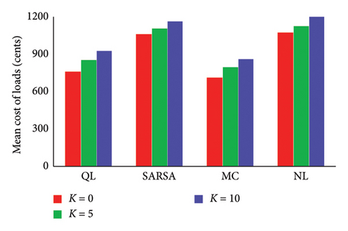
To illustrate the importance of selection parameter K, three different K, i.e., 0, 5, and 10 are considered for all the five customers inside the MG. It is worth noting that customers who prefer not to reduce their energy demand should opt for a higher dissatisfaction coefficient. In Figure 17 different algorithms and different respective K are shown. As it can be seen evidently as the K increase cost of customers increases dramatically. For example, when employing the QL algorithm for all loads, we observed a notable increase in the mean cost as the value of K varied. Specifically, the mean cost of loads rose by 12.11% when K increased from 0 to 5. Further elevating K to 10 resulted in a more substantial increase, reaching 8.42%. This trend indicates that higher values of K are associated with higher mean costs in the context of all the algorithms.

4.7. Comparison of Learning Algorithms

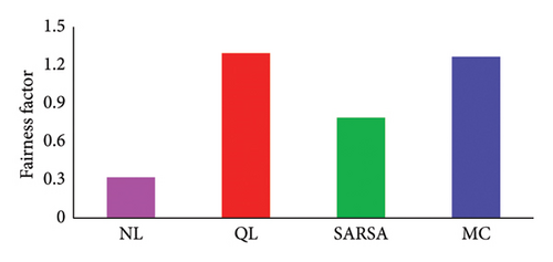
In this section, we used a fairness factor [19] in order to compare the results of different learning algorithms. The factor increases with a rise in the average profit of DERs, a decrease in the average cost for customers, or both. Consequently, a system that optimizes benefits for both customers and DERs achieves the highest fairness factor, ensuring fairness for all participating agents. We have computed this parameter for various algorithms, and the results are depicted in Figure 18. As shown, QL stands out with the best performance, achieving the highest value of 1.2643. Following that, we observe the MC algorithm with a value of 1.2358 and SARSA with a value of 0.7640. It is worth noting that in the absence of learning, the fairness factor was 0.30. Comparatively, when considering fairness improvement, the use of learning algorithms such as QL, MC, and SARSA demonstrated substantial increases in the fairness factor.

Another crucial aspect to consider is the simulation time. Table 10 provides simulation times for various learning algorithms, highlighting the superior performance of the QL algorithm. The QL algorithm stands out due to its exceptional efficiency and rapid adaptability to dynamic environments. Its ability to converge to optimal or near-optimal policies faster than other algorithms showcases remarkable computational efficiency, resulting in significant cost savings and resource conservation. This makes it a more economical solution for practical applications.

Table 10. Simulation time of different learning algorithms.

Algorithm	QL (s)	SARSA (s)	MC (s)
Simulation time	1483	4637	1879.74

Another essential factor is the memory required for the simulation, which depends on the dimensionality of the matrices utilized. It is evident that MC requires significantly more memory compared with QL. This difference arises from the larger data storage tables used in MC, as it stores entire episode trajectories, while QL updates its estimates incrementally during the learning process. Hence, QL is the preferred choice to select in terms of memory efficiency.

5. Conclusion

In this research, a decentralized energy management approach based on RL was implemented to oversee energy operations within the NEL. Within this framework, both energy producers and consumers were regarded as agents with the capacity to make decisions aimed at maximizing their profits. By employing a DA agent, the price of the internal market was determined, and any remaining unmet loads and surplus energy from producers were exchanged with the main grid. The result of the QL algorithm was compared with SARSA and MC. When comparing their results using real-world data, it became evident that the QL algorithm outperformed the other algorithms. Based on the fairness factor results, the performance of QL and MC are almost similar. However, considering QL’s lower computational complexity, reduced memory requirements, and faster execution compared to MC, it is recommended that QL be preferred for practical applications. This decentralized energy management approach can be used in the future net zero building to help in achieving net zero targets for smart cities by 2050.

Conflicts of Interest

The authors declare no conflicts of interest.

Funding

This research received no specific funding.

Open Research

Data Availability Statement

The data that support the findings of this study are available from the corresponding author upon reasonable request.

References

1 Liao Y., Transformation of Electric Power Grid Into Smart Grid, International Journal of Advance Innovations, Thoughts and Ideas. (2013) 02, no. 04, 76–81, https://doi.org/10.4172/2277-1891.1000149.
10.4172/2277-1891.1000149
Google Scholar
2 Lu D., Hu D., Yi F., Li J., and Yang Q., Optimal Selection Range of FCV Power Battery Capacity Considering the Synergistic Decay of Dual Power Source Lifespan, International Journal of Hydrogen Energy. (2023) 48, no. 36, 13578–13590, https://doi.org/10.1016/j.ijhydene.2022.12.135.
10.1016/j.ijhydene.2022.12.135
CAS Web of Science® Google Scholar
3 Marnay C., Chatzivasileiadis S., Abbey C. et al., Microgrid Evolution Roadmap, 2015 International Symposium on Smart Electric Distribution Systems and Technologies (EDST), September, 2015, 139–144, https://doi.org/10.1109/sedst.2015.7315197, 2-s2.0-84964412506.
10.1109/sedst.2015.7315197
Google Scholar
4 Ji Y., Wang J., Xu J., Fang X., and Zhang H., Real-Time Energy Management of a Microgrid Using Deep Reinforcement Learning, Energies. (2019) 12, no. 12, https://doi.org/10.3390/en12122291, 2-s2.0-85068375874.
10.3390/en12122291
Web of Science® Google Scholar
5 Abbasi A. R. and Baleanu D., Recent Developments of Energy Management Strategies in Microgrids: An Updated and Comprehensive Review and Classification, Energy Conversion and Management. (2023) 297, https://doi.org/10.1016/j.enconman.2023.117723.
10.1016/j.enconman.2023.117723
Web of Science® Google Scholar
6 Lee H. L. and Chun Y. H., Using Piecewise Linearization Method to PCS Input/Output-Efficiency Curve for a Stand-Alone Microgrid Unit Commitment, Energies. (2018) 11, no. 9, https://doi.org/10.3390/en11092468, 2-s2.0-85053917915.
10.3390/en11092468
Web of Science® Google Scholar
7 Hossain M. A., Pota H. R., Squartini S., and Abdou A. F., Modified PSO Algorithm for Real-Time Energy Management in Grid-Connected Microgrids, Renewable Energy. (2019) 136, 746–757, https://doi.org/10.1016/j.renene.2019.01.005, 2-s2.0-85060317723.
10.1016/j.renene.2019.01.005
Web of Science® Google Scholar
8 Kamarposhti M. A., Colak I., Shokouhandeh H., Iwendi C., Padmanaban S., and Band S. S., Optimum Operation Management of Microgrids With Cost and Environment Pollution Reduction Approach Considering Uncertainty Using Multi-Objective NSGAII Algorithm, IET Renewable Power Generation. (2022) 19, no. 1, https://doi.org/10.1049/rpg2.12579.
10.1049/rpg2.12579
Web of Science® Google Scholar
9 Sen S. and Kumar M., MPC Based Energy Management System for Grid-Connected Smart Buildings With EVs, 2022 IEEE IAS Global Conference on Emerging Technologies (GlobConET), 2022, Arad, Romania, 146–151.
Google Scholar
10 Vand B., Ruusu R., Hasan A., and Manrique Delgado B., Optimal Management of Energy Sharing in a Community of Buildings Using a Model Predictive Control, Energy Conversion and Management. (2021) 239, https://doi.org/10.1016/j.enconman.2021.114178.
10.1016/j.enconman.2021.114178
Web of Science® Google Scholar
11 Liu D., Zang C., Zeng P. et al., Deep Reinforcement Learning for Real-Time Economic Energy Management of Microgrid System Considering Uncertainties, Frontiers in Energy Research. (2023) 11, https://doi.org/10.3389/fenrg.2023.1163053.
10.3389/fenrg.2023.1163053
Web of Science® Google Scholar
12 Buşoniu L., Babuška R., and De Schutter B., Multi-agent Reinforcement Learning: An Overview, Studies in Computational Intelligence. (2010) 1, 183–221, https://doi.org/10.1007/978-3-642-14435-6_7, 2-s2.0-77956317028.
10.1007/978-3-642-14435-6_7
Google Scholar
13 Baldi S., Michailidis I., Ravanis C., and Kosmatopoulos E. B., Model-based and Model-free “Plug-and-play” Building Energy Efficient Control, Applied Energy. (2015) 154, 829–841, https://doi.org/10.1016/j.apenergy.2015.05.081, 2-s2.0-84930639824.
10.1016/j.apenergy.2015.05.081
Web of Science® Google Scholar
14 Hu X., Liu T., Qi X., and Barth M., Reinforcement Learning for Hybrid and Plug-In Hybrid Electric Vehicle Energy Management: Recent Advances and Prospects, IEEE Industrial Electronics Magazine. (2019) 13, no. 3, 16–25, https://doi.org/10.1109/mie.2019.2913015, 2-s2.0-85072611405.
10.1109/MIE.2019.2913015
Web of Science® Google Scholar
15 Silver D., Huang A., Maddison C. J. et al., Mastering the Game of Go with Deep Neural Networks and Tree Search, Nature. (2016) 529, no. 7587, 484–489, https://doi.org/10.1038/nature16961, 2-s2.0-84963949906.
10.1038/nature16961
CAS PubMed Web of Science® Google Scholar
16 Gu S., Holly E., Lillicrap T., and Levine S., Deep Reinforcement Learning for Robotic Manipulation with Asynchronous Off-Policy Updates, 2017 IEEE International Conference on Robotics and Automation (ICRA), 2017, May, 3389–3396, https://doi.org/10.1109/icra.2017.7989385, 2-s2.0-85027967014.
10.1109/icra.2017.7989385
Google Scholar
17 Darshi R., Shamaghdari S., Jalali A., and Arasteh H., Decentralized Energy Management System for Smart Microgrids Using Reinforcement Learning, IET Generation, Transmission & Distribution. (2023) 17, no. 9, 2142–2155, https://doi.org/10.1049/gtd2.12796.
10.1049/gtd2.12796
Web of Science® Google Scholar
18 Samadi E., Badri A., and Ebrahimpour R., Decentralized Multi-Agent Based Energy Management of Microgrid Using Reinforcement Learning, International Journal of Electrical Power & Energy Systems. (2020) 122, https://doi.org/10.1016/j.ijepes.2020.106211.
10.1016/j.ijepes.2020.106211
Web of Science® Google Scholar
19 Foruzan E., Soh L. K., and Asgarpoor S., Reinforcement Learning Approach for Optimal Distributed Energy Management in a Microgrid, IEEE Transactions on Power Systems. (2018) 33, no. 5, 5749–5758, https://doi.org/10.1109/tpwrs.2018.2823641, 2-s2.0-85052732987.
10.1109/TPWRS.2018.2823641
Web of Science® Google Scholar
20 Shouryadhar K., Chen C. N., and Chen Y. C., An Enhanced Reinforcement Learning Based Approach of Energy Management Optimization for Microgrids, 2022 IET International Conference on Engineering Technologies and Applications (IET-ICETA), October, 2022, 1–2, https://doi.org/10.1109/iet-iceta56553.2022.9971705.
10.1109/iet-iceta56553.2022.9971705
Google Scholar
21 Mughees N., Jaffery M. H., Mughees A., Ansari E. A., and Mughees A., Reinforcement Learning-Based Composite Differential Evolution for Integrated Demand Response Scheme in Industrial Microgrids, Applied Energy. (2023) 342, https://doi.org/10.1016/j.apenergy.2023.121150.
10.1016/j.apenergy.2023.121150
Web of Science® Google Scholar
22 Du Y. and Li F., Intelligent Multi-Microgrid Energy Management Based on Deep Neural Network and Model-Free Reinforcement Learning, IEEE Transactions on Smart Grid. (2020) 11, no. 2, 1066–1076, https://doi.org/10.1109/tsg.2019.2930299.
10.1109/TSG.2019.2930299
Web of Science® Google Scholar
23 Caralis G., Diakoulaki D., Yang P., Gao Z., Zervos A., and Rados K., Profitability of Wind Energy Investments in China Using a Monte Carlo Approach for the Treatment of Uncertainties, Renewable and Sustainable Energy Reviews. (2014) 40, 224–236, https://doi.org/10.1016/j.rser.2014.07.189, 2-s2.0-84906254388.
10.1016/j.rser.2014.07.189
Web of Science® Google Scholar
24 Thirunavukkarasu G. S., Seyedmahmoudian M., Jamei E., Horan B., Mekhilef S., and Stojcevski A., Role of Optimization Techniques in Microgrid Energy Management Systems—A Review, Energy Strategy Reviews. (2022) 43, https://doi.org/10.1016/j.esr.2022.100899.
10.1016/j.esr.2022.100899
Web of Science® Google Scholar
25 Heliocentris Energy Solutions Ag, New Energy Lab Instruction Manual. A Platform for Studying Energy Management, 2015.
Google Scholar
26 Sarker E., Seyedmahmoudian M., Jamei E., Horan B., and Stojcevski A., Optimal Management of Home Loads With Renewable Energy Integration and Demand Response Strategy, Energy. (2020) 210, https://doi.org/10.1016/j.energy.2020.118602.
10.1016/j.energy.2020.118602
Web of Science® Google Scholar
27 Akram U., Khalid M., and Shafiq S., Optimal Sizing of a Wind/Solar/Battery Hybrid Grid-Connected Microgrid System, IET Renewable Power Generation. (2018) 12, no. 1, 72–80, https://doi.org/10.1049/iet-rpg.2017.0010, 2-s2.0-85040325818.
10.1049/iet-rpg.2017.0010
Web of Science® Google Scholar
28 Roy S., Market Constrained Optimal Planning for Wind Energy Conversion Systems Over Multiple Installation Sites, IEEE Transactions on Energy Conversion. (2002) 17, no. 1, 124–129, https://doi.org/10.1109/60.986449, 2-s2.0-0036494122.
10.1109/60.986449
Web of Science® Google Scholar
29 El-Ela A. A. A., El-Seheimy R. A., Shaheen A. M., Wahbi W. A., and Mouwafi M. T., PV and Battery Energy Storage Integration in Distribution Networks Using Equilibrium Algorithm, Journal of Energy Storage. (2021) 42, https://doi.org/10.1016/j.est.2021.103041.
10.1016/j.est.2021.103041
Google Scholar
30 San Martín I., Ursúa A., and Sanchis P., Modelling of PEM Fuel Cell Performance: Steady-State and Dynamic Experimental Validation, Energies. (2014) 7, no. 2, 670–700, https://doi.org/10.3390/en7020670, 2-s2.0-84894558725.
10.3390/en7020670
Web of Science® Google Scholar
31 Degla A., Chikh M., Chouder A., Bouchafaa F., and Taallah A., Update Battery Model for Photovoltaic Application Based on Comparative Analysis and Parameter Identification of Lead–Acid Battery Models Behaviour, IET Renewable Power Generation. (2018) 12, no. 4, 484–493, https://doi.org/10.1049/iet-rpg.2017.0409, 2-s2.0-85043586063.
10.1049/iet-rpg.2017.0409
Web of Science® Google Scholar
32 León B. G. and Belardinelli F., Extended Markov Games to Learn Multiple Tasks in Multi-Agent Reinforcement Learning, arXiv preprint arXiv:2002.06000. (2020) .
Google Scholar
33 Rahimiyan M. and Mashhadi H. R., An Adaptive Q-Learning Algorithm Developed for Agent-Based Computational Modeling of Electricity Market, IEEE Transactions on Systems, Man, and Cybernetics, Part C (Applications and Reviews). (2010) 40, no. 5, 547–556, https://doi.org/10.1109/tsmcc.2010.2044174, 2-s2.0-77955828918.
10.1109/TSMCC.2010.2044174
Web of Science® Google Scholar
34 Sutton R. S. and Barto A. G., Reinforcement Learning: An Introduction, 2018, MIT Press.
Google Scholar
35 François-Lavet V., Fonteneau R., and Ernst D., How to Discount Deep Reinforcement Learning: Towards New Dynamic Strategies, arXiv preprint arXiv:1512.02011. (2015) .
Google Scholar
36 Rummery G. A. and Niranjan M., On-Line Q-Learning Using Connectionist Systems, 1994, 37, University of Cambridge, Department of Engineering, Cambridge, UK.
Google Scholar
37 Wang J., Wang Q., Zhou N., and Chi Y., A Novel Electricity Transaction Mode of Microgrids Based on Blockchain and Continuous Double Auction, Energies. (2017) 10, no. 12, https://doi.org/10.3390/en10121971, 2-s2.0-85044419097.
10.3390/en10121971
Web of Science® Google Scholar
38 Atwa Y. M., El-Saadany E. F., Salama M. M. A., and Seethapathy R., Optimal Renewable Resources Mix for Distribution System Energy Loss Minimization, IEEE Transactions on Power Systems. (2010) 25, no. 1, 360–370, https://doi.org/10.1109/tpwrs.2009.2030276, 2-s2.0-76649140102.
10.1109/TPWRS.2009.2030276
Web of Science® Google Scholar
39 Fang X., Zhao Q., Wang J., Han Y., and Li Y., Multi-Agent Deep Reinforcement Learning for Distributed Energy Management and Strategy Optimization of Microgrid Market, Sustainable Cities and Society. (2021) 74, https://doi.org/10.1016/j.scs.2021.103163.
10.1016/j.scs.2021.103163
PubMed Web of Science® Google Scholar
40 Crossing V., Weather Data Api, 2023.
Google Scholar

Citing Literature

All articles

Multiagent Energy Management System Design Using Reinforcement Learning: The New Energy Lab Training Set Case Study

Abstract

1. Introduction

2. Modeling Agents and Environment in the NEL

2.1. WT

2.2. PV Panels

2.3. FC

2.3.1. Thermodynamic Phenomena

2.3.2. Activation Phenomena

2.3.3. Concentration Phenomena

2.3.4. Double Layer Phenomena

2.3.5. Ohmic Phenomena

2.3.6. Peripheral Energy Consumption

2.4. Battery

2.4.1. Discharge Mode

2.4.2. Charge Mode

2.5. Loads

2.6. Environment Design

3. Energy Management Design Based on RL

3.1. Design of Agents’ Elements in Markov Game

3.1.1. Description of State Elements in the NEL Multiagent Environment

3.1.2. Description of Action Elements in the NEL Multiagent Environment

3.1.3. Description of Reward Elements in the NEL Multiagent Environment

3.1.3.1. Cumulative Reward: System-Wide Performance

3.2. Multiagent Reinforcement Learning (MARL) Algorithms: An Overview of QL, SARSA, and Monte Carlo

3.2.1. QL

3.2.2. SARSA

3.2.3. Monte Carlo

3.3. Hyperparameter Tunning

3.4. Double Auction Procedure for Energy Management of the NEL

4. Simulation and Results

4.1. Case Study

4.2. Configuration of MG

4.3. Sensitivity Analysis of Hyperparameters

4.4. Details of Markov Game Problem

4.5. Simulation Results and Analysis

4.6. Analysis of Dissatisfaction Factor on Cost of Customers

4.7. Comparison of Learning Algorithms

5. Conclusion

Conflicts of Interest

Funding

Open Research

Data Availability Statement

References

Citing Literature

Figures

References

Related

Information