Due to the intermittent and fluctuating nature of wind power generation, it is difficult to achieve the desired prediction accuracy for wind power prediction. For this reason, this paper proposes a combined prediction model based on the Pearson correlation coefficient method, multivariate variational mode decomposition (MVMD), African vultures optimization algorithm (AVOA) for leader–follower patterns, convolutional neural network (CNN), long short-term memory (LSTM), and attention mechanism (AM). Firstly, the Pearson correlation coefficient method is used to filter out the meteorological data with a strong relationship with wind power to establish the wind power prediction dataset; subsequently, MVMD is used to decompose the original data into multiple subsequences in order to handle the meteorological data better. Thereafter, the African vultures algorithm is used to optimize the hyperparameters of the CNN-LSTM algorithm, and the AM is added to increase the prediction effect, and the decomposed subsequences are predicted separately, and the predicted values of each subsequence are superimposed to obtain the final prediction value. Finally, the effectiveness of the model is verified using data from a wind farm in Shenyang. The results show that the MAE of the established MVMD-AVA-CNN-LSTM-AM model is 2.0467, and the MSE is 2.8329. Compared with other models, the prediction accuracy is significantly improved, and it had better generalization ability and robustness, and better generalization and robustness.

1. Introduction

In recent years, wind energy has emerged as a new type of renewable energy source that is clean and pollution-free. It can reduce environmental pollution caused by fossil fuels. At the same time, wind energy has become the fastest-growing sustainable energy source in the world because it is economical, convenient, and efficient [1–3]. However, as wind power continues to be connected to the grid, the problems caused by its intermittent and fluctuating nature are gradually becoming more prominent. Accurately predicting wind power can minimize operating costs and improve wind power utilization while ensuring reliability and stability [4–6]. At the same time, accurately predicting wind power also helps with electricity price forecasting [7] and improves the profits of wind power producers [8].

After the research of scholars, there are three commonly used methods for wind power prediction, which are the physical method [9], the statistical method [10], and the machine learning method [11].

The physical method is based on the geographic environment where the wind farms are located, considering the effects of atmospheric mesoscale modeling, to build a mathematical model [12]. Liao et al. [13] modeled the neighboring wind farms and local meteorological factors as a new form of graphs from a graph theoretical point of view, from which spatiotemporal correlations are captured. Physical methods are usually accompanied by huge amounts of data and require supercomputers for computation. This method is suitable for long-term forecasting with unsatisfactory short-term forecasting errors, while it is costly and complex to model [14].

The statistical methods include regression analysis [15], time series method [16], and Kalman filter [17], which builds a prediction model by finding the relationship between numerical weather data and power in wind farms [18], and the prediction results are drastically affected by historical data when using statistical methods. In the actual collection, many data are incomplete or abnormal because of communication failures or sensor problems. While the data are incomplete or abnormal, the prediction accuracy of the statistical method will be significantly and adversely affected. As a result, statistical methods are more straightforward and faster, but their prediction accuracy is limited in many ways.

The machine learning methods do not rely on predefined functional relationships between inputs and outputs. Instead, they leverage artificial intelligence techniques to learn from large volumes of historical data collected from wind farms. Through this process, they identify complex, nonlinear relationships among various weather and environmental factors, turbine conditions, and power output. By utilizing these learning methods, it is possible to predict the power output of different turbines and wind farms without needing to explicitly focus on factors such as the geographical location of the wind farm itself. Machine learning methods for predicting wind power include BPNN [19], SVM [20], and wavelet analysis [21].

At present, it is difficult to achieve good prediction results using a single method. At present, it is more common to use a hybrid of multiple methods to predict wind power. Zhang [22] et al. used CNN-SLTM for wind power prediction, Gao [23] et al. used PCA combined with CNN-GRU for prediction and achieved good results, and Yao [24] et al. used GS-GRU for wind speed prediction, and the results showed that they predicted the wind speed variation well. In order to improve the prediction accuracy, the use of the modal decomposition method to decompose the initial features has become a standard means of the research; Zhou [25] et al. used EMD combined with long short-term memory (LSTM) to predict wind power, Xu [26] et al. used VMD combined with ELM to achieve wind power prediction as well, and Zhang [27] et al. used VMD combined with TCN-BIGRU to predict wind power sufficiently as well. Good wind power prediction was also achieved. To further improve the prediction effect, hybrid models generally introduce heuristic algorithms to optimize the hyperparameters. Wei [28] et al. used IGWO to optimize the hyperparameters of the BP neural network and achieved good results. Xin [29] et al. used the IPSO algorithm to optimize the ELM and further improve the prediction effect. Wang et al. [30] used PSO to optimize the BP neural network and achieved better prediction results.

In this paper, we proposed an MVMD-AVOA-CNN-LSTM-AM model for wind power’s intermittent and fluctuating nature based on the Pearson correlation coefficient (PCC) method, multivariate variational mode decomposition (MVMD), African vultures optimization algorithm (AVOA) for leader–follower patterns, convolutional neural network (CNN), LSTM, and attention mechanism (AM).

At the beginning of the model construction, we used the PCC method to screen out the meteorological data closely related to wind power generation and established a wind power generation prediction dataset. Then, MVMD decomposes the original data into multiple subsequences for better meteorological data processing. Then, the AVOA is used to optimize the hyperparameters of the CNN-LSTM algorithm. The AM is added to enhance the prediction effect. The decomposed subsequences are predicted separately, and then the predicted values of each subsequence are superimposed to obtain the final prediction value. Finally, we used wind power data obtained from wind farms in Liaoning Province, China, for experiments to evaluate the performance of the prediction model.

This paper contains the following innovations:

1.
MVMD is introduced to decompose the data into multiple subsequences. Individual predictions are made for the decomposed subsequences, and the final prediction value is obtained by stacking the predicted values of each subsequence.
2.
The AVOA optimizes the hyperparameters of the CNN-LSTM algorithm to obtain better prediction results.
3.
Introducing an AM: The AM can automatically focus on the input data at key time steps, effectively handle long-term and short-term dependencies in time series data, and reduce the impact of redundant information, further improving the prediction results.

2. Data Preprocessing

2.1. PCC Method

PCC method is one of the common methods to measure the strength of the correlation between two variables and is widely used to measure the correlation between two variables. The PCC method evaluates the strength of the correlation between two variables based on the covariance matrix. When the correlation coefficient is closer to 1, it means that the two variables are positively correlated; when the correlation coefficient is closer to −1, it means that the two variables are negatively correlated. When the correlation coefficient is close to 0, it means that the correlation between the two variables is weak. Assuming that there are two variables X and Y, the formula for calculating the correlation coefficient between them can be expressed as follows:

()

where cov(X, Y) is the covariance of X and Y, and σ_X,σ_Y are the standard deviations of X and Y, respectively.

2.2. MVMD

MVMD can decompose weather data and wind power simultaneously, effectively linking the time and frequency domain relationships between weather data and wind power, effectively ensuring the consistency of the frequency scales of the decomposed modal books corresponding to the layers of modal classification with different features, and improving the stability and reconstruction accuracy of the decomposed signals.

The MVMD problem, i.e., under the finite bandwidth where each mode is a center frequency, searches for k modal functions that minimize the sum of the estimated bandwidths of all modes under the constraint that the sum of all modes is the original input signal. The steps by which MVMD can decompose the weather data and wind power simultaneously are as follows:

•
Step 1. Extract k multivariate oscillations u_k(t) in c input channels, i.e., x(t) = [x₁(t), x₂(t), ⋯, x_c(t)], such that
()
where u_k(t) = [u₁(t), u₂(t), ⋯, u_c(t)].
•
Step 2. Use the Hilbert transform to obtain the analytic signal for each oscillation in u_k(t). Use to denote the resolved signal of u_k(t), and then multiply it with the exponential term to adjust it to the corresponding center frequency ω_k(t). The bandwidth of u_k(t) can be predicted by the L₂ paradigm of the gradient function of the resolved . Then, the constrained variational function of the MVMD is given as follows:
()
where ∂_t is the partial derivative with respect to t, u_k(t) is the kth IMF component of the decomposition, and corresponds to the resolved signal for each oscillation of in channel c.
•
Step 3. The Lagrange multiplier λ and the quadratic penalty term α are introduced into the MVMD, where α ensures the accuracy of signal reconstruction in the presence of Gaussian noise, and the multiplier λ comes to ensure that the constraints are strictly satisfied, and the resulting augmented Lagrangian function is given as
()
•
Step 4. The above equation is solved using the alternate direction method of multipliers (ADMM) by iteratively updating u_k(t) and ω_k where the modal updating relationship can be calculated as
()

The center frequency update relationship can be calculated as

()

3. Theoretical Approach Background

3.1. CNN

The CNN is a kind of feed forward neural network with the characteristics of local connectivity and weight sharing. The CNN consists of input layer, convolutional layer, pooling layer, fully connected layer, and output layer.

The input layer can handle multidimensional data, the activation layer maps the results of the convolutional layer to a high-dimensional nonlinear space, the pooling layer downsamples the data to reduce the feature space and filter out the unimportant information, the fully connected layer is used to classify the results, and the output layer outputs the final result of the whole process.

The CNN layer is used to extract the implicit feature information of the input signal by using a convolutional kernel to perform the convolutional operation with the following equation:

()

where

is the ith feature region of the kth layer,

is the jth weight of the ith convolution kernel of the kth layer, M_i is the set of current feature inputs,

is the network bias term, and f is the activation function.

3.2. LSTM

Long short-term memory neural networks (LSTMs) are special RNNs, especially suitable for sequential sequence data processing, which solves the gradient vanishing and gradient explosion problems of traditional RNNs when dealing with long sequences, and the LSTM introduces a special kind of storage unit and gating mechanism to capture and deal with the long-term dependencies of ground in the sequence data more efficiently. Its structure is shown in Figure 1.

Details are in the caption following the image — **Figure 1**
Open in figure viewer PowerPoint

Structure of LSTM.

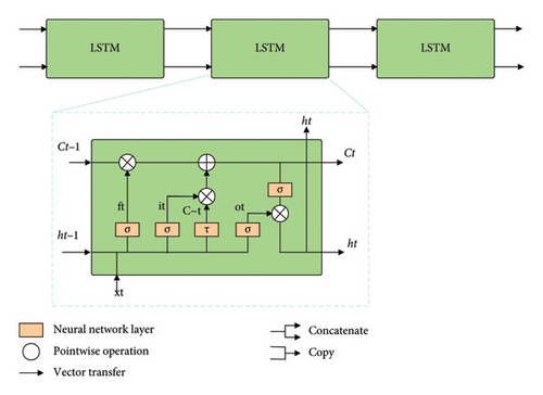
The neural network layer is used as a layer for learning. The pointwise operation performs point-by-point arithmetic operations. The vector transfer moves vectors in the direction of the arrows. The concatenate operation joins two vectors together. The copy operation duplicates a vector into two copies.

The core of LSTM is the cell state, and the long horizontal line across the top of the graph, which determines what information will be retained and what information will be forgotten, is denoted as C_t.

The LSTM implements three gate computations, the forgetting gate, the input gate, and the output gate, to protect and control the cell state.

The forgetting gate is responsible for deciding how much of the cell state from the previous moment is retained to the cell state at the current moment. Its formula is as follows:

()

The input gate is responsible for determining how much of the current moment’s input is retained to the current moment’s cell state and is formulated as follows:

()

The output gate is responsible for determining how many outputs are available from the cell state at the current moment and is formulated as follows:

()

3.3. AM

The CNN-LSTM model can effectively extract local global feature information; however, when dealing with longer sequences, there will still be some global correlation information that cannot be adequately captured.

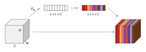
Therefore, this paper introduces the SE AM as shown in Figure 2, which adaptively recalibrates the channel-based feature responses by explicitly modeling the interdependencies between channels. Specifically, the importance level of each channel is automatically acquired by learning, and then the useful features are promoted, and the features that are not very useful for the current task are suppressed according to this importance level, in order to further enhance the model’s representational and modeling capabilities when dealing with sequential data.

Given an input with feature Channel Number c1, a feature with feature Channel Number c2 is obtained after a series of general transformations such as convolution. Then, the previously obtained feature is recalibrated by three operations of the SE module:

•
Step 1. Squeeze compression, which turns the two-bit feature of each channel into a real number, which characterizes the global distribution of the response over the feature channels, and is implemented using global flat global pooling, and the formula for global average pooling is as follows:
()
•
Step 2. Excitation excitation, the importance of each channel is predicted through fully connected layers. The first fully connected layer has C∗SERatio neurons with 1 × 1 × C inputs and 1 × 1 × C × SERadio outputs, which act as a dimensionality reduction. The second fully connected layer has C neurons with an input of 1 × 1 × C × SERadio and an output of 1 × 1 × C.
•
Step 3. Scale Scaling, consider the weights of the output of Excitation as the importance of each feature channel after feature selection, and then weight it to the previous features channel by channel by multiplication to complete the recalibration of the original features in the channel dimension.

3.4. AVOA

The AVOA simulates the foraging and navigational behaviors of African vultures. In the natural environment, vultures constantly fly long distances in search of food, and the most common flight mode for vultures is rotational flight. During foraging, sometimes several species of vultures move to the same food source and clash with each other. Weak vultures in hunger become more aggressive and increase their own chances of obtaining food by encircling and attacking stronger vultures, depleting their energy and making them fatigued. The African vultures algorithm is generally divided into two phases, exploration and exploitation, linked to the biological activities of African vultures that fly long distances in search of food and hover and clash near it. The specific process is illustrated in Figure 3 below.

•
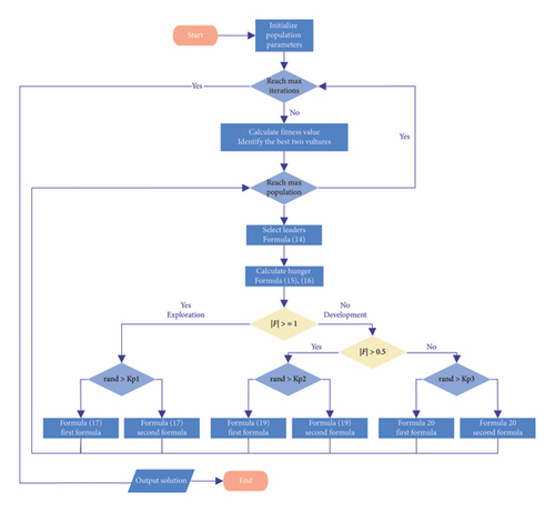
Step 1. After the start of the iteration, the vultures are grouped according to their quality, the vultures corresponding to the optimal solution are placed in the first group and the vultures corresponding to the suboptimal solution are placed in the second group. The rest of the vultures are placed in the third group and the selection of the vultures to follow is carried out according to the following equation.
()
where R(i) is the current individual learning, Best₁ denotes the best bald eagle, Best₂ denotes the second best bald eagle, and L is a user-defined parameter located in the range [0,1], which favors the population to search in the global range when L tends to 0 and favors the population to search in the local range when it tends to 1.
•
Step 2. Calculate the population hunger level
When the vultures have low hunger, they have enough strength to go farther to find food, and if the vultures have high hunger now, they will become more aggressive and therefore approach the vultures that have food. Based on the above behavior, we use the following equations to calculate the vulture’s hunger level.
()

()
where F represents the vulture’s hunger; I_i denotes the current number of iterations; M denotes the maximum number of iterations; and h, z, and k₁ are uniformly distributed random numbers between [−2, 2], [−1, 1], and [0, 1], respectively. w is a user-defined parameter controlling the probability that the algorithm will go into the exploratory mode in the final stage. When |F| ≥ 1, AVOA is in the exploratory phase, and when |F| < 1, AVOA is in the exploitation phase.
•
Step 3. When a vulture searches for food, it first takes some time to judge the surrounding environment and then finds the food after a long flight. In AVOA, the specific formula for the exploration phase is shown as follows:
()

()
where K_p1 is the exploration parameter set in advance, P(i + 1) is the vulture position vector in the next iteration, X is a constant, k₂ and k₃ are random numbers between [0, 1], and ub and lb are the upper and lower bounds of the optimization search, respectively.
•
Step 4. Development phase
When |F| is between 0.5 and 1, the AVOA enters the first stage of the development phase and executes the strategy of rotary flight, which is shown in the following equation:
()
where K_p2, k₄, and k₅ are random numbers between [0, 1].

When |F| is less than 0.5, the second stage of the development phase, i.e., the process of competition for food, is shown in the following equation:

()

where levy(d) denotes the levy flight operation and K_p3 is a random number between [0, 1].

3.5. Predictive Model Construction

Combining MVMD, CNN, LSTM, AM, and AOVA algorithm, this paper constructs the combined model, and its structure and flow are shown in Figure 4.

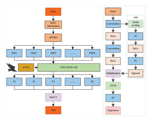
In order to mine the complex relationships in the weather data, the first step is to adopt the MVMD method to decompose the original weather data into submodalities with different frequencies. By adaptively decomposing the multivariate signals, the MVMD is able to efficiently extract the implicit features in the data, which can provide more stable input information for the subsequent prediction, thus better improving the accuracy.

To optimize the hyperparameters of the prediction model, we introduced the AVOA to adjust the learning rate and the number of nodes of the CNN and the LSTMN. AVOA is a heuristic algorithm based on the foraging behaviors of the vultures in the natural world, which has excellent global searching ability and convergence performance. The integration of AVOA with the CNN and LSTM facilitates the automatic search for the optimal model parameters, thereby enhancing the accuracy and the generalization capability of the prediction model.

Furthermore, the introduction of an AM into the prediction model is intended to enhance its accuracy. The AM has the capacity to selectively focus on the important parts of the input sequence that are relevant to the prediction task, thus enhancing the model’s ability to capture both local and global features.

4. Experimental Analysis

The programming language of the experimental environment in this paper is MATLAB, the version is MATLAB R2023b, the CPU is Intel i9-13900H, and the RAM size is 32.0 GB.

4.1. Data Preprocessing

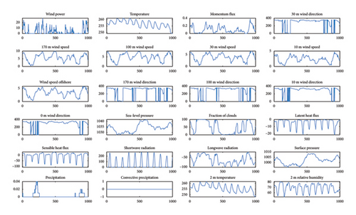
The wind power numerical weather prediction (NWP) dataset [31] is provided by the Public Science Data Center for Basic Disciplines in China. These datasets record data pertaining to a wind farm in Jilin Province, China, over the course of a year, encompassing wind power and momentum fluxes, temperature, barometric pressure, wind speed, and other relevant variables, with a time step of 15 min. The total number of valid data points is 35,136, and part of the data is shown in Figure 5.

The correlation between each meteorological data and wind power was analyzed using the PCC method to obtain a heat map as shown in Figure 6.

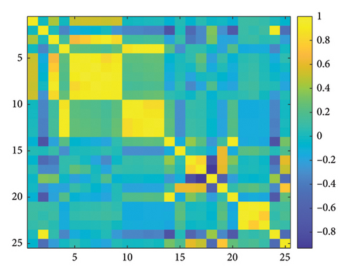
In the end, we chose the six meteorological data with higher correlation with wind power: momentum flux, 170 m wind speed, 100 m wind speed, 30 m wind speed, 10 m wind speed, and sea level wind speed.

We used min-max normalization to process the data to improve the prediction accuracy and accelerate the optimization of the model, the normalization function scales the data to [0, 1], and the function is defined as follows:

()

4.2. Data Segmentation and Evaluation Indicators

In order to better adapt to the training of the model, we chose 1000 data in January and divided them into training set, validation set, and test set according to 8:1:1.

At present, there is no uniform specific standard for the evaluation of the model, and the most commonly used evaluation indexes are mean absolute error (MAE) and root mean square error (RMSE) and their formulas are given as follows:

()

where n is the number of predicted points and x and y are the predicted and true values, respectively.

4.3. Decomposition Mode Selection (MVMD)

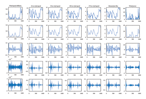
MVMD of weather data and predicted power is performed, with the center frequency method used to determine the optimal decomposition mode values. The decomposition mode center frequencies are displayed in Table 1. It is evident that excessive decomposition can lead to anomalous noise or mode overlap, while inadequate decomposition may result in undecomposed modes. The condition for determining mode overdecomposition is that adjacent modes possess analogous center frequency values. As can be seen in Table 1, this is the case for Modes 5 and 4. Therefore, the sequence is overdecomposed, and the optimal number of decompositions selected in this scheme is K = 4.

Table 1. Decomposed modal center frequency.

K	IMF1	IMF2	IMF3	IMF4	IMF5
K = 1	41.3211
K = 2	39.5649	6.7373
K = 3	38.7504	2.5193	1.2365
K = 4	38.2811	1.1224	2.7083	0.3019
K = 5	35.4812	3.1546	0.4450	1.0963	0.3417

The decomposition of momentum flux, 170 m wind speed, 100 m wind speed, 30 m wind speed, 10 m wind speed, sea level wind speed, and wind power are decomposed according to K = 4. The decomposition of each meteorological data set is illustrated in Figure 7.

4.4. Determine the Time Step

It is important to note that varying results may be obtained when employing different time steps for prediction. To address this, the LSTM model is utilized as the fundamental model to ascertain the input time step. The range of the step is designated in [1, 5], and the outcomes are presented in Figure 8 for various time steps, respectively.

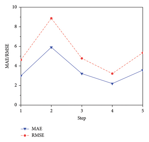
So the time step of the four models is chosen to predict the wind power.

4.5. MVMD and AM Validity Testing

In order to verify the effectiveness of MVMD and the AM, models were constructed for comparison with the prediction network. These comprised the AVOA-CNN-LSTM-AM and the MVMD-AVOA-CNN-LSTM models. The prediction results of these models are shown in Figure 9.

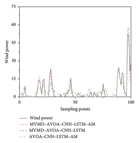
The results of the evaluation indicators are shown in Table 2.

Table 2. Comparison of model prediction results in validity experiments.

	MVMD-AVOA-CNN-LSTM-AM	MVMD-AVOA-CNN-LSTM	AVOA-CNN-LSTM-AM
MAE	2.0467	2.7688	2.6534
RMSE	2.8329	4.4246	3.6845

Then, we compared the prediction errors of the MVMD-AVOA-CNN-LSTM-AM, AVOA-CNN-LSTM-AM, and MVMD-AVOA-CNN-LSTM models to analyze the effects of MVMD and AM. The results are shown in Figure 10.

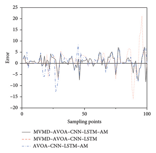
Subsequently, we conducted an in-depth analysis of the errors of the three models, and the results are shown in Figure 11. In ablation experiments, without the effect of the MVMD or AM mechanism, the errors are obviously more dispersed, and the results show that the MVMD-AVOA-CNN-LSTM-AM has a higher prediction accuracy.

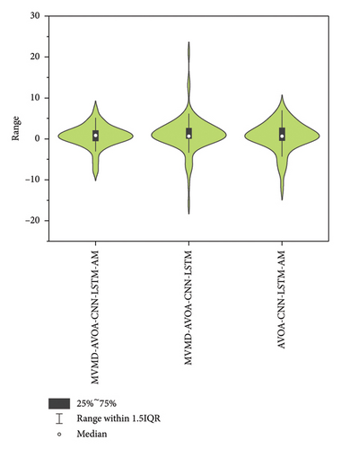
The error of MVMD-AVOA-CNN-LSTM-AM is relatively smaller and more concentrated. This proves that model fusion of MVMD and AM significantly improves the prediction results and improves the robustness and stability of the prediction model.

4.6. Comparison Experiment

To further verify the accuracy of the MVMD-AVOA-CNN-LSTM-AM prediction model, we compared it with BP model, GA-BP model, and MVMD-AVOA-CNN-GRU-AM model, whose prediction results are shown in Figure 12.

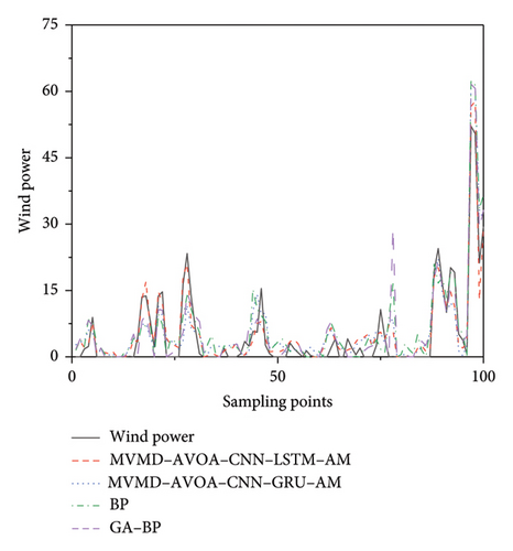
The results of the evaluation indicators are shown in Table 3.

Table 3. Comparison of model prediction results in comparative experiments.

	MVMD-AVOA-CNN-LSTM-AM	MVMD-AVOA-CNN-GRU-AM	BP	GA-BP
MAE	2.0467	3.0377	3.0586	2.6802
RMSE	2.8329	4.1536	4.3528	4.5094

Then, we analyzed the errors of four different models, and the error results are shown in Figure 13.

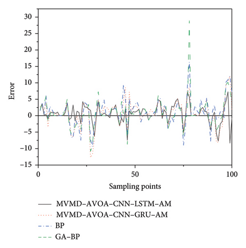
Subsequently, we conducted an in-depth analysis of the errors of the four models in the comparative experiment and obtained the violin diagram, as shown in Figure 14. The results show that the prediction accuracy of MVMD-AVOA-CNN-LSTM-AM is significantly higher.

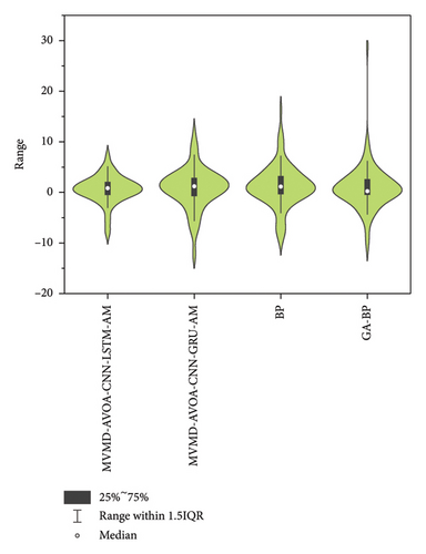
After comparison, we found that MVMD-AVOA-CNN-LSTM-AM has significantly better prediction results and is more stable and robust than models such as MVMD-AVOA-CNN-GRU-AM, BP, and GA-BP.

4.7. Universal Experiment

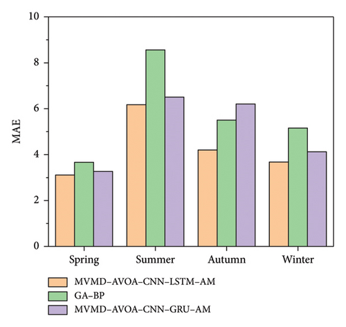
In order to verify the generalizability of the model, a test was conducted for each of the four seasons: spring, summer, autumn, and winter. The predicted MAEs for the four seasons are displayed in Figure 15.

In verifying the robustness and stability of the model, 10 experiments were conducted for different models, and the MAE of the prediction results obtained is displayed in Figure 16.

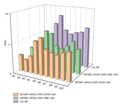
In a comprehensive comparison, we found that the MVMD-AVOA-CNN-LSTM-AM model has better prediction results and higher generalization and robustness of the model in multiple tests in all seasons.

5. Conclusions

In this paper, a novel wind power prediction model (MVMD-AVOA-CNN-LSTM-AM) is proposed, which integrates MVMD, the AVOA for leader–follower patterns, a CNN and a LSTM network, and an AM. Initially, the weather data are decomposed using the PCC method to extract the numerical MVMD algorithm that is more relevant to wind power to extract its main features. Subsequently, the AVOA is employed to enhance the learning rate, the number of nodes of the CNN, and the LSTM network to enhance the network’s capacity to process the weather data. Introducing an AM, which adaptively recalibrates channel-based feature responses by explicitly modeling interdependencies between channels and enhances the model’s prediction accuracy.

The model proposed in this paper can effectively deal with the nonstationarity and stochasticity of meteorological data, thus improving the accuracy and reliability of wind power prediction. The experimental results demonstrate that the model’s MAE is 2.0467, and the RMSE is 2.8329. A comparison with traditional prediction models reveals that the proposed model significantly improves prediction accuracy while exhibiting strong generalization capabilities and excellent model robustness. In the future, the team will continue to refine its work to enhance wind power prediction accuracy further. It is anticipated that this will provide a valuable reference point for related research in the future, including electricity price forecasting and power flow calculations.

Conflicts of Interest

The authors declare no conflicts of interest.

Funding

No funding was received for this research.

Open Research

Data Availability Statement

The data used to support the findings of this study are available at https://cstr.cn/16666.11.nbsdc.ky6qsoym.

References

1 Paris B., Vandorou F., Balafoutis A. T. et al., Energy Use in Greenhouses in the EU: A Review Recommending Energy Efficiency Measures and Renewable Energy Sources Adoption, Applied Sciences. (2022) 12, no. 10, https://doi.org/10.3390/app12105150.
10.3390/app12105150
Google Scholar
2 Aquilas N. A. and Atemnkeng J. T., Climate-related Development Finance and Renewable Energy Consumption in Greenhouse Gas Emissions Reduction in the Congo Basin, Energy Strategy Reviews. (2022) 44, https://doi.org/10.1016/j.esr.2022.100971.
10.1016/j.esr.2022.100971
Web of Science® Google Scholar
3 Li Z., Shen T., Yin Y., and Chen H. H., Innovation Input, Climate Change, and Energy-Environment-Growth Nexus: Evidence from OECD and Non-OECD Countries, Energies. (2022) 15, no. 23, https://doi.org/10.3390/en15238927.
10.3390/en15238927
Web of Science® Google Scholar
4 Pijnenburg P., Cao B., Chang L., Kilpatrick R., and Levy T., A Post-forecast Weighing Algorithm to Improve Wind Power Forecasting Capabilities, IET Renewable Power Generation. (2023) 17, no. 2, 296–304, https://doi.org/10.1049/rpg2.12597.
10.1049/rpg2.12597
Web of Science® Google Scholar
5 Chen Y., Yu S., Islam S., Lim C. P., and Muyeen S. M., Decomposition-based Wind Power Forecasting Models and Their Boundary Issue: An In-Depth Review and Comprehensive Discussion on Potential Solutions, Energy Reports. (2022) 8, 8805–8820, https://doi.org/10.1016/j.egyr.2022.07.005.
10.1016/j.egyr.2022.07.005
Web of Science® Google Scholar
6 Li M., Yang M., Yu Y., Li P., and Wu Q., Short-Term Wind Power Forecast Based on Continuous Conditional Random Field, IEEE Transactions on Power Systems. (2024) 39, no. 1, 2185–2197, https://doi.org/10.1109/TPWRS.2023.3270662.
10.1109/TPWRS.2023.3270662
Web of Science® Google Scholar
7 Maciejowska K., Nitka W., and Weron T., Enhancing Load, Wind and Solar Generation for Day-Ahead Forecasting of Electricity Prices, Energy Economics. (2021) 99, https://doi.org/10.1016/j.eneco.2021.105273.
10.1016/j.eneco.2021.105273
Web of Science® Google Scholar
8 Xiao D., Chen H., Cai W., Wei C., and Zhao Z., Integrated Risk Measurement and Control for Stochastic Energy Trading of a Wind Storage System in Electricity Markets, Protection and Control of Modern Power Systems. (2023) 8, no. 1, https://doi.org/10.1186/s41601-023-00329-3.
10.1186/s41601-023-00329-3
Web of Science® Google Scholar
9 Aerts F., Lanzilao L., and Meyers J., Bayesian Uncertainty Quantification Framework for Wake Model Calibration and Validation with Historical Wind Farm Power Data, Wind Energy. (2023) 26, no. 8, 786–802, https://doi.org/10.1002/we.2841.
10.1002/we.2841
Web of Science® Google Scholar
10 Chen Z., Wang J., Guo J. et al., Statistical Method of Low Efficiency Wind Turbine Generating Wind Power Curve Based on Operating Data, Journal of Physics: Conference Series. (2022) 2218, no. 1, https://doi.org/10.1088/1742-6596/2218/1/012062.
10.1088/1742-6596/2218/1/012062
Google Scholar
11 Liu S., Wang L., Jiang H., Liu Y., and You H., Wind Farm Energy Storage System Based on Cat Swarm Optimization–Backpropagation Neural Network Wind Power Prediction, Frontiers in Energy Research. (2022) 10, https://doi.org/10.3389/fenrg.2022.850295.
10.3389/fenrg.2022.850295
Web of Science® Google Scholar
12 Chang W.-Y., A Literature Review of Wind Forecasting Methods, Journal of Power and Energy Engineering. (2014) 02, no. 04, 161–168, https://doi.org/10.4236/jpee.2014.24023.
10.4236/jpee.2014.24023
Google Scholar
13 Liao W., Wang S., Bak-Jensen B., Radhakrishna Pillai J., Yang Z., and Liu K., Ultra-short-term Interval Prediction of Wind Power Based on Graph Neural Network and Improved Bootstrap Technique, Journal of Modern Power Systems and Clean Energy. (2023) 11, no. 4, 1100–1114, https://doi.org/10.35833/mpce.2022.000632.
10.35833/MPCE.2022.000632
Web of Science® Google Scholar
14 Chandra D. R., Kumari M. S., and Sydulu M., A Detailed Literature Review on Wind Forecasting, Paper Presented at the 2013 International Conference on Power, Energy and Control (ICPEC), February 2013.
Google Scholar
15 Mogos A. S., Salauddin M., Liang X., and Chung C. Y., An Effective Very Short-Term Wind Speed Prediction Approach Using Multiple Regression Models, IEEE Canadian Journal of Electrical and Computer Engineering. (2022) 45, no. 3, 242–253, https://doi.org/10.1109/ICJECE.2022.3152524.
10.1109/ICJECE.2022.3152524
Web of Science® Google Scholar
16 Jin J., Ye L., Li J. et al., Wind and Photovoltaic Power Time Series Data Aggregation Method Based on an Ensemble Clustering and Markov Chain, CSEE Journal of Power and Energy Systems. (2022) 8, no. 3, 757–768, https://doi.org/10.17775/CSEEJPES.2020.03700.
10.17775/CSEEJPES.2020.03700
Web of Science® Google Scholar
17 Li D., Yu X., Liu S., Dong X., Zang H., and Xu R., Wind Power Prediction Based on PSO-Kalman, Energy Reports. (2022) 8, 958–968, https://doi.org/10.1016/j.egyr.2022.02.077.
10.1016/j.egyr.2022.02.077
Web of Science® Google Scholar
18 Wang B., Wang T., Yang M., Han C., Huang D., and Gu D., Ultra-Short-Term Prediction Method of Wind Power for Massive Wind Power Clusters Based on Feature Mining of Spatiotemporal Correlation, Energies. (2023) 16, no. 6, https://doi.org/10.3390/en16062727.
10.3390/en16062727
PubMed Web of Science® Google Scholar
19 Ofori-Ntow Jnr E., Ziggah Y. Y., Rodrigues M. J., and Relvas S., A Hybrid Chaotic-Based Discrete Wavelet Transform and Aquila Optimisation Tuned-Artificial Neural Network Approach for Wind Speed Prediction, Results in Engineering. (2022) 14, https://doi.org/10.1016/j.rineng.2022.100399.
10.1016/j.rineng.2022.100399
PubMed Google Scholar
20 You H., Bai S., Wang R. et al., New PSO-SVM Short-Term Wind Power Forecasting Algorithm Based on the CEEMDAN Model, Journal of Electrical and Computer Engineering. (2022) 2022, 1–9, https://doi.org/10.1155/2022/7161445.
10.1155/2022/7161445
Web of Science® Google Scholar
21 Dhiman H. S., Deb D., and Guerrero J. M., On Wavelet Transform Based Convolutional Neural Network and Twin Support Vector Regression for Wind Power Ramp Event Prediction, Sustainable Computing: Informatics and Systems. (2022) 36, https://doi.org/10.1016/j.suscom.2022.100795.
10.1016/j.suscom.2022.100795
Web of Science® Google Scholar
22 Zhang J., Zhao Z., Yan J., and Cheng P., Ultra-Short-Term Wind Power Forecasting Based on CGAN-CNN-LSTM Model Supported by Lidar, Sensors. (2023) 23, no. 9, https://doi.org/10.3390/s23094369.
10.3390/s23094369
Web of Science® Google Scholar
23 Gao J., Ye X., Lei X., Huang B., Wang X., and Wang L., A Multichannel-Based CNN and GRU Method for Short-Term Wind Power Prediction, Electronics. (2023) 12, no. 21, https://doi.org/10.3390/electronics12214479.
10.3390/electronics12214479
Web of Science® Google Scholar
24 Yao H., Tan Y., Hou J., Liu Y., Zhao X., and Wang X., Short-Term Wind Speed Forecasting Based on the EEMD-GS-GRU Model, Atmosphere. (2023) 14, no. 4, https://doi.org/10.3390/atmos14040697.
10.3390/atmos14040697
Web of Science® Google Scholar
25 Zhou Z., Sun S., and Gao Y., Short-term Wind Power Prediction Based on EMD-LSTM, 2023 IEEE 3rd International Conference on Power, Electronics and Computer Applications (ICPECA), April 2023, 802–807, https://doi.org/10.1109/ICPECA56706.2023.10076173.
10.1109/ICPECA56706.2023.10076173
Google Scholar
26 Xu T., Du Y., Li Y., Zhu M., and He Z., Interval Prediction Method for Wind Power Based on VMD-ELM/ARIMA-ADKDE, IEEE Access. (2022) 10, 72590–72602, https://doi.org/10.1109/ACCESS.2022.3189477.
10.1109/ACCESS.2022.3189477
Web of Science® Google Scholar
27 Zhang Y., Zhang L., Sun D., Jin K., and Gu Y., Short-Term Wind Power Forecasting Based on VMD and a Hybrid SSA-TCN-BiGRU Network, Applied Sciences. (2023) 13, no. 17, https://doi.org/10.3390/app13179888.
10.3390/app13179888
Google Scholar
28 Wei L., Xv S., and Li B., Short-term Wind Power Prediction Using an Improved Grey Wolf Optimization Algorithm with Back-Propagation Neural Network, Clean Energy. (2022) 6, no. 2, 288–296, https://doi.org/10.1093/ce/zkac011.
10.1093/ce/zkac011
Web of Science® Google Scholar
29 Xin Ju, ShangKe L., YanLi X., and Ye W., Prediction Model for Cost Data of a Power Transmission and Transformation Project Based on Pearson Correlation Coefficient–IPSO–ELM, Clean Energy. (2021) 5, no. 4, 756–764, https://doi.org/10.1093/ce/zkab052.
10.1093/ce/zkab052
Google Scholar
30 Wang C.-H., Zhao Q., and Tian R., Short-Term Wind Power Prediction Based on a Hybrid Markov-Based PSO-BP Neural Network, Energies. (2023) 16, no. 11, https://doi.org/10.3390/en16114282.
10.3390/en16114282
PubMed Web of Science® Google Scholar
31 Sun Y., Wind Power Numerical Weather Prediction-NWP Dataset. (V1). Hohai University [Creation Institution], 2022-12-19, National Basic Science Data Center.
Google Scholar

Citing Literature

All articles

Short-Term Wind Power Prediction Based on MVMD-AVOA-CNN-LSTM-AM

Abstract

1. Introduction