State estimation is a challenging problem, particularly in distribution grids that have unique characteristics compared with transmission grids. Conventional methods that solve the state estimation problem at the transmission level require the grid to be observable, which does not apply to distribution grids. To make the distribution grid observable, researchers resort to pseudomeasurements, which are inaccurate. Also, the high integration of renewable energy introduces uncertainty, making the Distribution System State Estimation (DSSE) problem even more complex. This work proposes a deep neural network approach that solves the DSSE problem in unobservable distribution grids without employing erroneous pseudomeasurements. We create a dataset that emulates real-life scenarios of diverse operating conditions with distributed generation. We then subject the neural network to multiple test scenarios featuring noisier measurements and bad data to evaluate the robustness of our algorithm. We test our approach on three networks. Results demonstrate that our method efficiently solves the DSSE problem—which cannot be solved using conventional methods—and detects and mitigates bad data, further enhancing the reliability of the state estimation results.

1. Introduction

Distribution systems differ from transmission systems by having a low X/R ratio, high unobservability, and a radial or weakly meshed topology. In addition, the penetration of renewable energy resources and distributed generation (DG) renders the generation less predictable. Hence, the Distribution System State Estimation (DSSE) problem has garnered considerable attention since the 1990s [1, 2]. Initially, researchers adopted the state estimation (SE) methods that are used in transmission systems to distribution systems. For example, the weighted least squares (WLS) method based on node voltages [3, 4] or branch currents [5], the least absolute value (LAV) method [6], and the generalized maximum likelihood (GML) approach [7]. However, WLS requires observability, LAV is computationally expensive and sensitive to measurement uncertainty, and GML is sensitive to parameter selection [8]. Consequently, techniques applied in transmission system SE (TSSE) prove ineffective in addressing the DSSE problem.

Observability analysis is carried out prior to SE, to ensure that the available measurements are sufficient to estimate the state of the system [9]. Compared with transmission grids, distribution grids have fewer installed measurements. To address the unobservability issue, pseudomeasurements are employed [10]. These are generated from historical, standard load, or weather data and thus are highly inaccurate. Probabilistic or statistical-based methods are used to generate these pseudomeasurements and handle their errors, for example, Gaussian mixture models [11], correlation analysis [12], and multivariate Gaussian modeling [13]. However, these pseudomeasurements, which are prone to inaccuracies, introduce accumulating errors into the analysis. Inaccurate input data, thus, lead to erroneous results, raising concerns about the effectiveness of the algorithms that depend on pseudomeasurements.

To address the uncertainty introduced by renewable energy integration, researchers are solving the DSSE problem in the presence of DGs. For instance, forecasting-aided DSSE is explored in [14] using GML and in [15] using L₁ regularization; optimal meter placement in active distribution grids is studied in [16], and pseudomeasurement generation with high DG penetration is studied in [17]. Also, [18] proposes models of photovoltaic arrays to be integrated within the network model, while [19] proposes an approach to generate pseudomeasurements for an active distribution grid.

Another problem that affects SE, in general, is bad data in measurements [20, 21]. Bad data are measurements that suffer from anomalies due to communication or meter errors. In [22], a Lagrangian-based approach is employed to identify bad data. In [23], L₁-norm is used to identify corrupted measurements and estimate the states. However, the L₁ penalty function is susceptible to outliers that have large magnitudes. The authors in [24] propose a statistical approach based on iterative reweight least squares and an improved alternating direction method of multipliers approach. Also, Ref. [25] formulates a phasor measurement unit (PMU)–based SE as a quadratic programming problem and solves it in a decentralized way to maintain privacy between operators.

However, the aforementioned methods are computationally expensive, particularly in scenarios with high dimensions. Moreover, the DSSE is a nonlinear problem whose complexity increases with the increase of renewable energy integration, and thus, traditional methods cannot handle this problem and are prone to introducing simplifications or guessing initial conditions. This leads the algorithm to either getting stuck in local optima or failing to converge.

In response to these challenges, researchers started exploring artificial intelligence (AI) algorithms to solve power system problems. These algorithms shift the computational burden to an offline stage, for example, solar energy forecasting [26–28] and load and generation forecasting [29–33]. In particular, for DSSE problems, examples include integrating AI algorithms with traditional algorithms such as [34] that employs a neural network to initialize the Gauss–Newton method [35] that proposes a neural network to generate pseudomeasurements, and [36] that uses a nonlinear autoregressive exogenous algorithm to predict the load and feed it back into the state estimator.

Another research path is to solve the DSSE problem using standalone AI methods. For instance, the authors in [37] adopted a Bayesian inference approach for unobservable distribution systems via deep learning. Autoencoders are studied in [38] to ensure two-way communication with unobservable distribution grids. The authors in [39, 40] introduce a physics-informed neural network that integrates the topology of the grid to solve the DSSE problem. Also, in [41], the authors propose a physics-guided approach that captures temporal features. The authors in [42, 43] propose state estimators based on graph neural networks to incorporate the topology of the grid in the model. These approaches showcase the AI potential to revolutionize the field and overcome the limitations posed by traditional methods.

Although these methods have achieved impressive results, the reviewed papers suffer from at least one of the following problems:

•
Some methods rely on pseudomeasurements, with errors up to 50%, to compensate for the unobservability issue, e.g., [34, 36, 37, 39, 41–43]. This practice leads to inaccurate results following the garbage-in garbage-out concept, raising concerns about the reliability of the proposed algorithms.
•
Several papers do not explicitly discuss whether their algorithms can handle bad data [34, 35, 38, 40, 42, 43], which restricts the practical deployment of the proposed methods. Also, these are not thoroughly verified against outliers or practical anomalies, which could limit the applicability of the algorithms in scenarios where data may experience anomalies.

This work proposes a deep learning approach that solves the DSSE problem in scenarios characterized by a scarcity of measurements, without relying on pseudomeasurements, which cannot be performed using conventional SE techniques. The contributions are threefold:

1.
We propose a deep neural network approach to solve the DSSE problem without resorting to erroneous pseudomeasurements. Our algorithm handles the limited measurements and the inherent unobservability of distribution grids. It is applicable in real time to cater to the need to frequently solve the DSSE problem. Our approach also handles the added complexity introduced by DG, showcasing its robustness in dynamically evolving grid environments.
2.
To validate the real-world applicability and robustness of our methodology, rigorous testing has been conducted under diverse conditions. We assess the algorithm performance given (a) noisier data and (b) bad data, ensuring that our approach remains effective even with less-than-ideal data conditions.
3.
Addressing a critical aspect often overlooked in similar studies, we show that bad data detection can be used to identify erroneous measurements. We propose a systematic approach for managing and mitigating the impact of bad data on the estimation process. This testing reinforces the algorithm’s reliability for practical scenarios.

The remainder of this manuscript is divided as follows. Section 2 formally defines the SE problem. Section 3 presents the approach used for creating the dataset. Section 4 details the methodology. Section 5 presents the results and discusses them. Finally, Section 6 concludes this paper.

2. Problem Statement

SE is a data processing algorithm that converts meter measurements and other data into an estimate of the state vector [44]. The state vector consists of the voltage magnitudes and phase angles in static SE, which can be used to calculate all variables of interest in a power system. Numerous algorithms have been proposed over the last 5 decades to solve the SE problem, mainly on the transmission level.

The measurement vector z, which includes m measurements, is defined as follows:

()

where z = [z₁, z₂, …, z_m] is the set of m measurements, x = [x₁, x₂, …, x_n] is a vector denoting n system states, composed of voltage magnitudes and phase angles, h(x) is a nonlinear function of x, and e is a vector denoting the measurement noise that is usually assumed to follow a Gaussian distribution with a zero mean and a covariance matrix

being the variance of z_i [9].

Generally, measurements include active and reactive power flows, power injections, complex phasor voltages, and current measurements. These measurements are taken from sensors and smart meters placed on the grid. For the SE to estimate the complete state of the grid, the grid must be observable. The grid observability is determined by the numbers, types, and locations of the available measurements. While there are usually enough redundant measurements installed in transmission grids to make them observable, that is not the case for distribution grids. Additionally, communication errors, topology changes, and faulty measurements may exacerbate the unobservability problem in distribution grids, resulting in cases where traditional SE cannot be carried out. In such cases, the system may need to be divided into isolated observable subsystems to achieve an incomplete estimate of the system state.

One major difference between TSSE and DSSE is that the approximations that allow TSSE to be linearized do not apply to DSSE. As such, the function h(x) is nonlinear in DSSE. Moreover, distribution networks are often unobservable and thus rely on pseudomeasurements that are generated using historical data, standard load profiles, or weather data to make the grid observable.

Thus, DSSE does not have an algebraic solution. It is solved numerically. The WLS method is used to minimize the impact of the noise, by minimizing the following objective function:

()

Usually, equation (2) is solved using the Gauss–Newton method [9]. However, this method is sensitive to initialization, computationally expensive, and not guaranteed to converge.

In this manuscript, we use five types of measurements, whose relations with the state variables are determined by the following equations:

•
Voltage magnitude at bus i: V_i.
•
Real and reactive power injections at bus i.
()

()
•
Real and reactive power flows from bus i to bus j:
()

()
where θ_ij = θ_i − θ_j, θ_i being the phase angle at bus i, G_ij + jB_ij is the ij^th element of the complex bus admittance matrix, g_ij + jb_ij is the admittance of the series branch connecting buses i and j, and g_si + jb_si is the admittance of the shunt branch connected at bus i.

3. Creating the Dataset

The existing datasets suffer from significant limitations. In [37, 38, 41–43], the datasets rely on pseudomeasurements generated from historical data, introducing an additional layer of uncertainty. The dataset used in [39] also depends on pseudomeasurements and incorporates μPMU measurements that are assumed to be noise-free, resulting in an idealistic approach. In addition, [40] assumes noiseless measurements from PMUs. These assumptions do not reflect practical scenarios, reducing the robustness and generalizability of the proposed estimation methods. The datasets are summarized in Table 1.

Table 1. Summary of datasets and their limitations.

Reference	Limitations
[37, 38, 41–43]	Reliance on pseudomeasurements
[39]	Noise-free μPMUs
[40]	Noise-free PMUs

Given these shortcomings and the lack of public frameworks, we create a new dataset that emulates real-life scenarios to train and test the neural network. This dataset dictates the variations in the states of the distribution grid in response to variations in generation and load, to provide a realistic representation of diverse operating conditions in power grids. We use the 18-, 85-, and 141-bus cases from MATPOWER 7.1 [45].

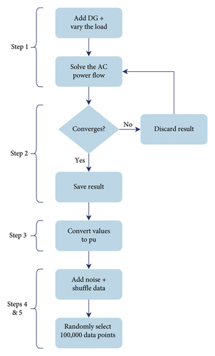
In Step 1, we introduce generation at 15% of the buses in each grid and vary the generation levels to emulate fluctuations in renewable energy sources, which are highly sensitive to weather conditions. This value is chosen arbitrarily and results in 3, 12, and 22 DG locations for each of the three aforementioned grids, respectively. We also vary the load at different buses between 50% and 200% of the original MATPOWER load values. This range was chosen to represent typical load variations in real-world power grids, where demand can fluctuate from half to double the base value, depending on the time of the day, weather conditions, and user behavior. This guarantees that we capture both under- and over-demand scenarios, to expose the neural network to a wide range of operating conditions. Then, we solve the AC power flow problem for each generation and load variation.

For example, for the 18-bus system, we add two constant active and reactive power generators, to emulate photovoltaic generators, at Buses 4 and 9 and a generator with automatic voltage regulation at Bus 21, as shown in Figure 1. The chosen measurements for the 18-bus system are the following:

•
Voltage measurement at bus: 50
•
Power injection measurement at bus: 51
•
Power flow measurements (from–to): 1–20, 2-3, 4-5, and 21–23, which represent 30% of the power flow measurements at one side, making the grid unobservable.

Details are in the caption following the image — **Figure 1**
Open in figure viewer PowerPoint

Measurement distribution for the 18-bus system.

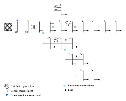
This measurement distribution is also shown in Figure 1. We highlight that this distribution cannot be used with conventional SE approaches. In traditional SE methodologies, observability of the entire grid is a prerequisite, a condition not met by the presented measurement distribution.

In Step 2, we check for convergence at every data instance: If the algorithm converges, then the result is saved, else it is discarded.

In Step 3, we convert all the values (except the angles) to the per-unit system. In Step 4, we emulate real measurements by adding Gaussian noise to the chosen measurements, with zero mean and the following standard deviations [9]:

•
0.004 pu for voltage measurements
•
0.01 pu for power injection measurements
•
0.008 pu for power flow measurements

In Step 5, we shuffle the data and randomly select 100,000 data points to train and test the neural network. The algorithm is summarized as a flowchart in Figure 2.

We replicate the same approach for the 85- and 141-bus systems while introducing variable generators at 15% of the buses and maintaining a consistent measurement distribution of 1 voltage measurement, 1 power injection measurement, and 30% of the power flow measurements.

4. Methodology

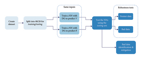
This section provides an overview of the proposed approach to address the DSSE problem. Initially, the neural network architecture is presented, followed by the description of robustness tests and the method for mitigating bad data. The diagram in Figure 3 summarizes the process, which is implemented for three distinct bus systems.

4.1. Neural Network

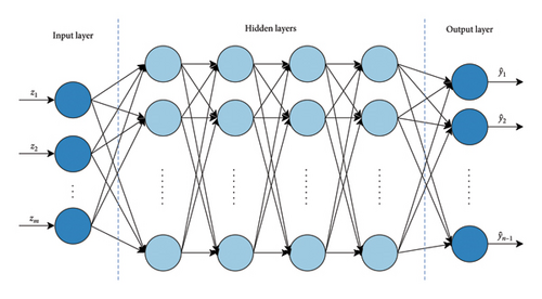
In this paper, we use a deep feedforward neural network that consists of one input layer, 4 hidden layers with the rectified linear unit (ReLU) as an activation function, and one output layer, without an activation function. For every grid topology, we build a dedicated neural network: one neural network to predict V and one to predict θ.

In every case, the inputs consist of m measurements, ranging from z₁ to z_m, depending on the grid size. The outputs consist of n − 1 state variables, representing voltage magnitudes and phase angles, with n being the number of buses. We predict n − 1 variables because the slack bus is predetermined, then its voltage magnitude and phase angle are already known, and thus, there is no need to include them in the neural network for prediction. The neural network architecture is shown in Figure 4.

For every neural network model, we perform data split to ensure effective training, validation, and testing. We divide the dataset into two parts: 80% is allocated to the training dataset and 20% is allocated to the testing dataset, which is reserved for evaluating the model’s performance after training. Within the training dataset, we further extract 20% of the data to create a separate validation set. This validation dataset plays a crucial role during the training process by helping monitor the model’s performance on unseen data, preventing overfitting, and guiding hyperparameter tuning. We note that, instead of predicting the angles, we predict the sine of the angles, i.e., sin(θ). This step serves as a preprocessing measure, to scale the output angles between −1 and 1. The angles can be recovered in postprocessing by applying an inverse sine operation since the sign is preserved. The chosen loss function is the mean squared error (MSE), formulated as follows:

()

where y_i is the ground truth vector. It is V for the first neural network and θ for the second;

is the predicted vector. It is

for the first neural network and

for the second.

The neural network is trained while employing the Adam optimizer with a learning rate set at 1e − 03, and the training process spans 200 epochs. The hyperparameters are summarized in Table 2.

Table 2. Parameters of the neural network.

Parameter	Value
Number of hidden layers	4
Number of neurons per hidden layer	Case specific
Train/test ratio	80%/20%
Validation split	20% (of the training set)
Optimizer	Adam
Learning rate	1e − 03
Number of epochs	200
Batch size	64
Loss function	MSE
Activation function	ReLU

4.2. Testing the Robustness of the Neural Network

After the neural network learns the mapping between the input measurements and the output states, we perform several test scenarios to verify its robustness.

4.2.1. Noisier Data

In this scenario, we assume that we have measurements with higher noise levels attributed to communication anomalies or extreme weather events. The measurement distribution remains consistent with the one outlined in Section 3, but we introduce additional noise in three steps: 2σ, 3σ, and 4σ. This noise is applied to all data points of the testing dataset, which consists of 20,000 data points. Then, based on these noisier measurements, we evaluate the performance of the previously trained neural network, without initiating a retraining process. This evaluation provides insights into the network’s robustness under conditions of added noise, mirroring potential challenges posed by external factors in practical applications.

4.2.2. Bad Data

In this scenario, we assume that we have bad data resulting from meter or communication errors. The measurement distribution remains consistent with the one outlined in Section 3, but we further corrupt the data by adding 10σ in three stages: We assume first that 10% of the measurements are bad data, followed by 20% and finally, 30%. This corruption is applied to the testing dataset, which consists of 20,000 data points, to emulate the presence of bad measurements. Then, based on these measurements, we evaluate the performance of the previously trained neural network, without initiating a retraining process. This evaluation provides valuable insights into the network’s resilience and effectiveness in handling bad data, a crucial aspect in practical applications where erroneous measurements are a prevalent challenge.

4.3. Bad Data Identification and Mitigation

The process of mitigating bad data is crucial in ensuring accurate SE results, particularly in distribution grids. To this end, since there is a scarcity of meters and sensors in distribution grids, we refrain from removing the bad measurement(s) once identified. Instead, we propose an alternative approach to minimize the impact of bad data on the accuracy of the problem.

After computing the voltage magnitudes and phase angles, denoted by and , respectively, we proceed to calculate the measurements using equations (3)–(6). This step enables the determination of the corresponding residual for each measurement, which indicates the discrepancy between the calculated values and the actual values.

Once a faulty measurement is identified, we do not simply remove it. Instead, we compute its value using equations (3)–(6) and replace it in the previous data input vector. Then, using the pretrained neural network, we estimate the new states and test the accuracy of the updated estimation. This approach ensures that the SE problem remains well posed and that the faulty measurement does not introduce additional errors into the system. By adopting this strategy, we achieve a more robust and reliable SE algorithm, even in the presence of bad data, making it well suited for real-world applications.

5. Results and Discussion

In this section, we present the findings of our study and provide a detailed discussion of our results. We first demonstrate the algorithm on the 18-bus system and then extend it to the 85- and 141-bus systems. Simulations were performed on the free version of Google Colaboratory, using the TensorFlow [46] platform.

5.1. 18-Bus System Demo

For the 18-bus system, we build a neural network, train it, and test it using the dataset generated in Section 3. Following the measurement distribution also presented in Section 3, the input vector z_NN consists of the values of V₅₁, P₅₁, Q₅₁, P₁₋₂₀, Q₁₋₂₀, P₂₋₃, Q₂₋₃, P₄₋₅, Q₄₋₅, P₂₁₋₂₃, and Q₂₁₋₂₃. The neural network has 4 hidden layers, with 16 neurons each. The output layer consists of n − 1 = 17 voltage magnitudes. We calculate 17 voltage magnitudes because the magnitude of the slack bus, in this case, Bus 51, is known beforehand. After several simulations, the average testing error, using the MSE formula defined in (7), is 6.03e − 07, as shown in Table 3. Furthermore, the average simulation time to calculate one data point is 67 ms, also shown in Table 3.

Table 3. Simulation results for voltage magnitudes and phase angles for the 3 test cases.

Case	Variable	MSE	Time (in ms)
18-bus	V	6.03e − 07	67
18-bus	θ	1.81e − 07	62

85-bus	V	3.15e − 07	64
85-bus	θ	6.12e − 08	65

141-bus	V	5.11e − 07	67
141-bus	θ	5.94e − 08	68

A similar neural network architecture is used to calculate the sine of the phase angles, except the neural network is now trained for different outputs. The same measurements are used as inputs. Results are also summarized in Table 3.

Furthermore, for the 18-bus case, the neural network is compared with the conventional SE method. We use the SE module of pandapower [47], which in turn uses the WLS method. To perform the WLS method, we provide the following measurements:

•
Voltage measurement at bus: 50; this is similar to the one chosen for the neural network.
•
Power injection measurement at bus: 51; this is also similar to the one chosen for the neural network.
•
Thirty percent of the power flow measurements, as given in the case of the neural network. But, with 30% only, the grid is unobservable; thus, the WLS method cannot be performed (for the WLS method to work, we should have at least 2n − 1 = 35 interdependent measurements available). Therefore, we increase the number of measurements to make the grid observable. The remaining 70% power flow measurements are given as pseudomeasurements.

We refer to these measurements as z_WLS. Similar to the neural network, Gaussian noise is used with zero mean, and the same standard deviations are provided in Section 3, except for the pseudomeasurements, which are generated with a higher standard deviation of 0.064. As for the neural network, we provide the algorithm with the measurements listed as z_NN, for the same data instance. We compare the MSE of the WLS method with that of the neural network method, for the same data instance. Results are summarized in Table 4.

Table 4. Comparing WLS with neural network for the 18-bus system.

Case	Variable	MSE of classic SE	MSE of proposed method
18-bus	V	4.96e − 05	1.53e − 07
18-bus	θ	1.74e − 05	1.42e − 07

Table 4 shows that our approach outperforms the classic SE, based on the WLS method, in both cases. We note that despite unobservability, our proposed approach consistently delivers superior results compared with the conventional SE method.

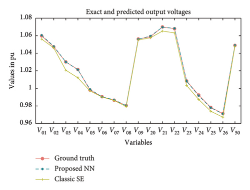
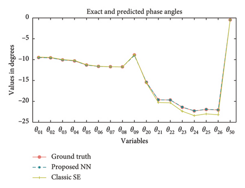
Moreover, Figure 5 shows the graphical representation of the errors between the estimated states obtained through our neural network and the conventional WLS method when compared with the true system states, for one data instance of the 18-bus system. This graph illustrates that the states estimated by the neural network closely follow the ground truth states, reaffirming the accuracy of our approach. In contrast, the WLS-calculated values deviate from the true states in multiple instances, displaying larger errors.

5.2. Comparison With State-of-the-Art Methods

For the 85-bus system, we also use a neural network with 4 hidden layers, but this time, every layer has 64 neurons. The rest of the parameters are the same as the ones for the 18-bus system. Also, one neural network is trained for predicting voltage magnitudes, and another is trained for predicting phase angles. Results are summarized in Table 3.

Table 3 indicates that the errors for the 85-bus system are 3.15e − 07 and 6.12e − 08. Both values present an improvement when compared with [37], having an error of 4.46e − 06, and [38], having an error in the order of 10⁻², as shown in Table 5. We note that both [37, 38] conducted their analyses on the 85-bus system. Our method thus outperforms cutting-edge methods presented in the literature.

Table 5. Comparison with state-of-the-art methods.

Case	Algorithm	MSE
85-bus	[37]	4.46e − 06
	[38]	In the order of 10⁻²
	Proposed method	3.15e − 07 and 6.12e − 08

141-bus	[38]	In the order of 10⁻²
141-bus	Proposed method	5.11e − 07 and 5.94e − 08

For the 141-bus case, the hidden layers are also 4, but with 128 neurons each. This is done to compensate for the larger dimensionality of the bigger grids. Results are also summarized in Table 3. For the 141-bus system, the errors are 5.11e − 07 and 5.94e − 08 for predicting the voltage magnitudes and phase angles, respectively. These values present an improvement over [38] whose method presents an error in the order of 10⁻², as shown in Table 5. Our method thus outperforms cutting-edge AI methods presented in the literature.

Table 3 shows that our approach performs very well, under noisy measurements and unobservability. In addition, our method strategically shifts the computational burden to an offline stage. Thus, we evaluate the simulation time when this algorithm is used online to calculate a single output. In every case, the simulation time spent to calculate one data instance is in the millisecond range, making our approach a practical alternative in scenarios where real-time computations are essential. Moreover, even with larger grid topologies, the neural network still achieves impressive results, in terms of both accuracy and simulation time, solidifying its practical scalability across diverse power system configurations.

5.3. Noisier Data

In this scenario, we subject the method to rigorous testing. Given the trained neural network, we test the algorithm using noisier data. That is, we add 2σ, 3σ, and 4σ to the measurements available in the testing dataset and check the performance of the neural network without retraining it. Results are summarized in Table 6.

Table 6. Noisier data results for all cases.

Case	Variable	Original MSE	MSE with 2σ	MSE with 3σ	MSE with 4σ
18-bus	V	6.03e − 07	8.52e − 07	1.25e − 06	2.33e − 06
18-bus	θ	1.81e − 07	3.49e − 07	7.17e − 07	9.84e − 07

85-bus	V	3.15e − 07	4.65e − 07	7.20e − 07	9.48e − 07
85-bus	θ	6.12e − 08	8.21e − 08	1.14e − 07	3.84e − 07

141-bus	V	5.11e − 07	7.17e − 07	9.07e − 07	1.08e − 06
141-bus	θ	5.94e − 08	6.31e − 08	9.92e − 08	2.56e − 07

For example, when calculating θ for the 141-bus system, the error increases from 6.31e − 08 for noise with a 2σ standard deviation to 2.56e − 07 for 4σ. These results show that the proposed approach can still be used with noisier measurements, despite being scarce. Also, the accuracy remains higher than the conventional SE method which requires a larger volume of data. This emphasizes the method’s efficacy in scenarios with limited availability of precise measurements.

5.4. Bad Data

In this scenario, we further corrupt the data by adding 10σ to the testing dataset in three stages: We assume first that 10% of the measurements are bad data, followed by 20% and then 30%. We test the neural network without retraining it. Results are summarized in Table 7.

Table 7. Bad data results for all cases.

Case	Variable	Original MSE	MSE with 10% bad data	MSE with 20% bad data	MSE with 30% bad data
18-bus	V	6.03e − 07	1.18e − 06	3.34e − 05	2.26e − 04
18-bus	θ	1.81e − 07	6.32e − 06	9.75e − 05	1.08e − 04

85-bus	V	3.15e − 07	1.06e − 06	3.60e − 05	2.37e − 05
85-bus	θ	6.12e − 08	6.82e − 06	1.47e − 05	7.37e − 05

141-bus	V	5.11e − 07	5.91e − 06	2.88e − 05	3.82e − 04
141-bus	θ	5.94e − 08	5.58e − 06	8.12e − 05	5.42e − 04

Results illustrate the robustness of our approach, even when confronted with 10% of the measurements classified as bad data, e.g., an error of 5.58e − 06 for the 141-bus system, when calculating θ. Our approach also performs better than the conventional SE method without bad data. As expected, the performance gradually declines to 8.12e − 05 and 5.42e − 04 when the percentage of bad data increases to 20% and 30%, respectively. This highlights the resilience of our neural network-based solution in the face of bad data.

5.5. Bad Data Identification and Mitigation

In this scenario, we assume we have 1 bad measurement corrupted by 10σ, identify it, and alleviate its effect on the accuracy of the results. After computing the estimated voltage magnitudes and phase angles , we calculate the power flow measurements using equation (5) or (6) and get the corresponding residual for each measurement. Results are shown in Table 8. A careful analysis of these residuals shows that the bad measurement in this scenario is P₄₋₅.

Table 8. Residuals before and after fixing the bad measurement.

Power flow measurements	Initial residuals	Residuals after mitigating bad measurements
P₁₋₂₀	1.3647	1.4204
Q₁₋₂₀	0.8782	0.2346
P₂₋₃	1.9200	0.7367
Q₂₋₃	2.2108	0.4556
P₄₋₅	5.5896	1.5030
Q₄₋₅	1.0927	0.0189
P₂₁₋₂₃	0.8540	0.4642
Q₂₁₋₂₃	0.7611	0.1976

Rather than deleting this power flow measurement, its value is calculated using equation (5). This calculated value is then used to estimate the new and , effectively reducing the impact of the faulty measurement on the overall DSSE accuracy. The resulting residuals are presented in Table 8. We can observe that the residual values have dropped from 5.5896 to 1.5030, indicating a significant improvement in the accuracy of the DSSE. These corrective steps demonstrate the effectiveness of our approach in handling bad data and improving the robustness of the DSSE algorithm.

5.6. Computational Complexity

The WLS method solves the SE problem by iteratively solving a nonlinear optimization problem. Its computational complexity depends on the size of the power grid, the number of measurements, and the iterative steps required to converge. The computational complexity of WLS is O(k(mn² + n³)), where k is the number of iterations to reach convergence, m is the number of measurements, and n is the number of states [9, 37]. In particular, with a dense Jacobian matrix and the use of the Newton–Raphson algorithm, the complexity is approximated to O(n³).

On the other hand, our proposed algorithm uses a feedforward neural network with 4 hidden layers where the number of neurons per layer is adaptable to the grid size. Each neuron in a layer performs a weighted sum of inputs from the previous layer and applies the ReLU activation function. Thus, the number of operations depends on the number of neurons in each layer and the number of inputs from the previous layer [48]. The computational complexity of our method is O(h²), where h denotes the number of neurons per hidden layer. This complexity reduction shows the superiority of our algorithm, which offers a scalable and efficient alternative to traditional WLS methods. We also note that the neural network approach shifts the computational burden to an offline stage and can be easily applied in real time.

5.7. Discussion

The findings presented in this study offer compelling insights into the robustness of our proposed approach to solving the DSSE problem. Several key observations and contributions can be highlighted:

•
Our approach solves the DSSE problem with high accuracy, despite the grid being highly unobservable, as shown in Table 3. We recall that we only have 1 voltage measurement, 1 power injection measurement, and 30% of the power flow measurements. We do not use any pseudomeasurements. Moreover, the simulation time is in the order of milliseconds, even for the large 141-bus network. This enables frequent solving of the DSSE problem, enhancing its practicality for operators.
•
We compare our proposed approach with the WLS method, as shown in Table 4 and Figure 5. We show that the proposed method is more accurate despite having fewer inputs than WLS. Also, the WLS method cannot be performed using the same number of measurements provided to the neural network.
•
We also conducted a comprehensive comparison of our proposed approach against several state-of-the-art methods, as detailed in Table 5. Results demonstrate that the performance of our method consistently surpasses the existing AI techniques.
•
Table 6 shows that the neural network is robust to additional noise. This is attributed to the fact that the neural network was trained on a large dataset, making it more immune to noise and enhancing its generalization capabilities.
•
Table 7 shows that the neural network maintains good accuracy, with 10% of bad data. The performance, however, starts declining as more data are corrupted.
•
Table 8 shows that we can compute the value of the faulty measurement instead of removing it, to minimize the effect of bad data on the SE results.

6. Conclusion

In this paper, we have introduced a deep feedforward neural network approach to address the DSSE problem in the presence of DG. We created a new dataset that captures real-world scenarios and includes both generation and load variations. We have provided a solution that tackles the fundamental issue of unobservability in distribution grids without relying on pseudomeasurements. Results demonstrate that our algorithm surpasses both traditional and existing neural network-based methods, achieving superior performance with fewer measurements while maintaining high accuracy even under noisy conditions. Moreover, our method exhibits remarkable robustness when subjected to diverse test scenarios. It accurately predicts voltage magnitudes and phase angles across different grid topologies, during millisecond-scale time, aligning with the operational requirements of power systems. Additionally, our approach to handling bad data further strengthens the reliability of the SE process. These results suggest that the proposed algorithm is a practical and efficient solution for real-world DSSE applications in power systems with distributed energy resources.

Future work will focus on exploring the impact of false data injection (FDI) attacks on the presented approach. These attacks are known as adversarial attacks, which compromise the SE results by subtly manipulating sensor data in a way that would bypass bad data detection algorithms. These FDI attacks alter the perceived state of the power system, potentially causing significant damage. Previous research has tackled FDI attacks on conventional SE methods and explored protective measures for securing the power system against such threats [49, 50]. Building on this foundation, we also aim to explore our approach to incorporate dynamic SE at the distribution level, where real-time challenges are more pronounced. This extension opens paths for safeguarding future power grids against sophisticated adversarial attacks.

Disclosure

This manuscript is part of a master’s thesis at the Lebanese American University, under the supervision of Dr. Harag Margossian. This manuscript, however, advances the research presented in the thesis significantly.

Conflicts of Interest

The authors declare no conflicts of interest.

Funding

This research received no grant funding from any agency.

Open Research

Data Availability Statement

The data used in this study are available upon request.

References

1 Roytelman I. and Shahidehpour S., State Estimation for Electric Power Distribution Systems in Quasi Real-Time Conditions, IEEE Transactions on Power Delivery. (1993) 8, no. 4, 2009–2015, https://doi.org/10.1109/61.248315, 2-s2.0-0027679096.
10.1109/61.248315
Web of Science® Google Scholar
2 Baran M. E. and Kelley A. W., State Estimation for Real-Time Monitoring of Distribution Systems, IEEE Transactions on Power Systems. (1994) 9, no. 3, 1601–1609, https://doi.org/10.1109/59.336098, 2-s2.0-0028480212.
10.1109/59.336098
Web of Science® Google Scholar
3 Li K., State Estimation for Power Distribution System and Measurement Impacts, IEEE Transactions on Power Systems. (1996) 11, no. 2, 911–916, https://doi.org/10.1109/59.496174, 2-s2.0-0030149336.
10.1109/59.496174
Web of Science® Google Scholar
4 Therrien F., Kocar I., and Jatskevich J., A Unified Distribution System State Estimator Using the Concept of Augmented Matrices, IEEE Transactions on Power Systems. (2013) 28, no. 3, 3390–3400, https://doi.org/10.1109/tpwrs.2013.2248398, 2-s2.0-84881023696.
10.1109/TPWRS.2013.2248398
Web of Science® Google Scholar
5 Baran M. E. and Kelley A. W., A Branch-Current-Based State Estimation Method for Distribution Systems, IEEE Transactions on Power Systems. (1995) 10, no. 1, 483–491, https://doi.org/10.1109/59.373974, 2-s2.0-0029254783.
10.1109/59.373974
Web of Science® Google Scholar
6 Göl M. and Abur A., LAV Based Robust State Estimation for Systems Measured by PMUs, IEEE Transactions on Smart Grid. (2014) 5, no. 4, 1808–1814, https://doi.org/10.1109/tsg.2014.2302213, 2-s2.0-84903266505.
10.1109/TSG.2014.2302213
Web of Science® Google Scholar
7 Zhao J., Zhang G., Scala M. L., and Wang Z., Enhanced Robustness of State Estimator to Bad Data Processing Through Multiinnovation Analysis, IEEE Transactions on Industrial Informatics. (2017) 13, no. 4, 1610–1619, https://doi.org/10.1109/tii.2016.2626782, 2-s2.0-85029714800.
10.1109/TII.2016.2626782
Web of Science® Google Scholar
8 Dehghanpour K., Wang Z., Wang J., Yuan Y., and Bu F., A Survey on State Estimation Techniques and Challenges in Smart Distribution Systems, IEEE Transactions on Smart Grid. (2019) 10, no. 2, 2312–2322, https://doi.org/10.1109/tsg.2018.2870600, 2-s2.0-85053331840.
10.1109/TSG.2018.2870600
Web of Science® Google Scholar
9 Abur A. and Exposito A. G., Power System State Estimation: Theory and Implementation, 2004, CRC Press.
10.1201/9780203913673
Google Scholar
10 Ghosh A. K., Lubkeman D. L., and Jones R. H., Load Modeling for Distribution Circuit State Estimation, IEEE Transactions on Power Delivery. (1997) 12, no. 2, 999–1005, https://doi.org/10.1109/61.584427, 2-s2.0-0031119329.
10.1109/61.584427
Web of Science® Google Scholar
11 Singh R., Pal B. C., and Jabr R. A., Statistical Representation of Distribution System Loads Using Gaussian Mixture Model, IEEE Transactions on Power Systems. (2010) 25, no. 1, 29–37, https://doi.org/10.1109/tpwrs.2009.2030271, 2-s2.0-76649139141.
10.1109/TPWRS.2009.2030271
Web of Science® Google Scholar
12 Nguyen D. T., Modeling Load Uncertainty in Distribution Network Monitoring, IEEE Transactions on Power Systems. (2015) 30, no. 5, 2321–2328, https://doi.org/10.1109/tpwrs.2014.2364819, 2-s2.0-85027916970.
10.1109/TPWRS.2014.2364819
Web of Science® Google Scholar
13 Arefi A., Ledwich G., and Behi B., An Efficient DSE Using Conditional Multivariate Complex Gaussian Distribution, IEEE Transactions on Smart Grid. (2015) 6, no. 4, 2147–2156, https://doi.org/10.1109/tsg.2014.2385871, 2-s2.0-85027949749.
10.1109/TSG.2014.2385871
Web of Science® Google Scholar
14 Zhao J., Zhang G., Dong Z. Y., and La Scala M., Robust Forecasting Aided Power System State Estimation Considering State Correlations, IEEE Transactions on Smart Grid. (2018) 9, no. 4, 2658–2666, https://doi.org/10.1109/tsg.2016.2615473, 2-s2.0-85041995108.
10.1109/TSG.2016.2615473
Web of Science® Google Scholar
15 Dutta R., Geetha S. J., Chakrabarti S., and Sharma A., An L-1 Regularized Forecasting-Aided State Estimator for Active Distribution Networks, IEEE Transactions on Smart Grid. (2022) 13, no. 1, 191–201, https://doi.org/10.1109/tsg.2021.3115816.
10.1109/TSG.2021.3115816
Web of Science® Google Scholar
16 Liu J., Ponci F., Monti A., Muscas C., Pegoraro P. A., and Sulis S., Optimal Meter Placement for Robust Measurement Systems in Active Distribution Grids, IEEE Transactions on Instrumentation and Measurement. (2014) 63, no. 5, 1096–1105, https://doi.org/10.1109/tim.2013.2295657, 2-s2.0-84898810563.
10.1109/TIM.2013.2295657
Web of Science® Google Scholar
17 Margossian H. Z., Iterative State Estimation With Weight Tuning and Pseudo-Measurement Generation, IEEE Systems Journal. (2021) 15, no. 3, 3165–3172, https://doi.org/10.1109/jsyst.2021.3060072.
10.1109/JSYST.2021.3060072
Web of Science® Google Scholar
18 Fang Z., Lin Y., Song S., Li C., Lin X., and Chen Y., State Estimation for Situational Awareness of Active Distribution System With Photovoltaic Power Plants, IEEE Transactions on Smart Grid. (2021) 12, no. 1, 239–250, https://doi.org/10.1109/tsg.2020.3009571.
10.1109/TSG.2020.3009571
Web of Science® Google Scholar
19 Liu J., Singh R., and Pal B. C., Distribution System State Estimation With High Penetration of Demand Response Enabled Loads, IEEE Transactions on Power Systems. (2021) 36, no. 4, 3093–3104, https://doi.org/10.1109/tpwrs.2020.3047269.
10.1109/TPWRS.2020.3047269
Web of Science® Google Scholar
20 Merrill H. M. and Schweppe F. C., Bad Data Suppression in Power System Static State Estimation, IEEE Transactions on Power Apparatus and Systems. (1971) no. 6, 2718–2725, https://doi.org/10.1109/tpas.1971.292925, 2-s2.0-0015159258.
10.1109/TPAS.1971.292925
Google Scholar
21 Handschin E., Schweppe F. C., Kohlas J., and Fiechter A., Bad Data Analysis for Power System State Estimation, IEEE Transactions on Power Apparatus and Systems. (1975) 94, no. 2, 329–337, https://doi.org/10.1109/t-pas.1975.31858, 2-s2.0-0016480359.
10.1109/T-PAS.1975.31858
Web of Science® Google Scholar
22 Caro E., Conejo A. J., and Minguez R., Decentralized State Estimation and Bad Measurement Identification: An Efficient Lagrangian Relaxation Approach, IEEE Transactions on Power Systems. (2011) 26, no. 4, 2500–2508, https://doi.org/10.1109/tpwrs.2011.2157367, 2-s2.0-80054917612.
10.1109/TPWRS.2011.2157367
Web of Science® Google Scholar
23 Kekatos V. and Giannakis G. B., Distributed Robust Power System State Estimation, IEEE Transactions on Power Systems. (2013) 28, no. 2, 1617–1626, https://doi.org/10.1109/tpwrs.2012.2219629, 2-s2.0-84883177193.
10.1109/TPWRS.2012.2219629
Web of Science® Google Scholar
24 Ho C. H., Wu H., Chan S., and Hou Y., A Robust Statistical Approach to Distributed Power System State Estimation With Bad Data, IEEE Transactions on Smart Grid. (2020) 11, no. 1, 517–527, https://doi.org/10.1109/tsg.2019.2924496, 2-s2.0-85068583652.
10.1109/TSG.2019.2924496
Web of Science® Google Scholar
25 Lin C., Wu W., and Guo Y., Decentralized Robust State Estimation of Active Distribution Grids Incorporating Microgrids Based on PMU Measurements, IEEE Transactions on Smart Grid. (2020) 11, no. 1, 810–820, https://doi.org/10.1109/tsg.2019.2937162.
10.1109/TSG.2019.2937162
Web of Science® Google Scholar
26 Hussain A., Khan Z. A., Hussain T., Ullah F. U. M., Rho S., and Baik S. W., A Hybrid Deep Learning-Based Network for Photovoltaic Power Forecasting, Complexity. (2022) 2022, no. 1, https://doi.org/10.1155/2022/7040601.
10.1155/2022/7040601
Web of Science® Google Scholar
27 Munsif M., U Min Ullah F., Ullah Khan S., Khan N., Wook Baik S., and Baik S. W., CT-NET: A Novel Convolutional Transformer-Based Network for Short-Term Solar Energy Forecasting Using Climatic Information, Computer Systems Science and Engineering. (2023) 47, no. 2, 1751–1773, https://doi.org/10.32604/csse.2023.038514.
10.32604/csse.2023.038514
Google Scholar
28 Khan Z. A., Hussain T., and Baik S. W., Dual Stream Network With Attention Mechanism for Photovoltaic Power Forecasting, Applied Energy. (2023) 338, https://doi.org/10.1016/j.apenergy.2023.120916.
10.1016/j.apenergy.2023.120916
Web of Science® Google Scholar
29 Khan Z. A., Khan S. A., Hussain T., and Baik S. W., DSPM: Dual Sequence Prediction Model for Efficient Energy Management in Micro-Grid, Applied Energy. (2024) 356, https://doi.org/10.1016/j.apenergy.2023.122339.
10.1016/j.apenergy.2023.122339
Web of Science® Google Scholar
30 Khan Z. A., Hussain T., Ullah W., and Baik S. W., A Trapezoid Attention Mechanism for Power Generation and Consumption Forecasting, IEEE Transactions on Industrial Informatics. (2024) 20, no. 4, 5750–5762, https://doi.org/10.1109/tii.2023.3335453.
10.1109/TII.2023.3335453
Web of Science® Google Scholar
31 Khan Z. A., Hussain T., Ullah A., Rho S., Lee M., and Baik S. W., Towards Efficient Electricity Forecasting in Residential and Commercial Buildings: A Novel Hybrid CNN With a LSTM-AE Based Framework, Sensors. (2020) 20, no. 5, https://doi.org/10.3390/s20051399.
10.3390/s20051399
Web of Science® Google Scholar
32 Khan Z. A., Hussain T., and Baik S. W., Boosting Energy Harvesting via Deep Learning-Based Renewable Power Generation Prediction, Journal of King Saud University Science. (2022) 34, no. 3, https://doi.org/10.1016/j.jksus.2021.101815.
10.1016/j.jksus.2021.101815
Web of Science® Google Scholar
33 Khan Z. A., Hussain T., Haq I. U., Ullah F. U. M., and Baik S. W., Towards Efficient and Effective Renewable Energy Prediction via Deep Learning, Energy Reports. (2022) 8, 10230–10243, https://doi.org/10.1016/j.egyr.2022.08.009.
10.1016/j.egyr.2022.08.009
Web of Science® Google Scholar
34 Zamzam A. S., Fu X., and Sidiropoulos N. D., Data-Driven Learning-Based Optimization for Distribution System State Estimation, IEEE Transactions on Power Systems. (2019) 34, no. 6, 4796–4805, https://doi.org/10.1109/tpwrs.2019.2909150.
10.1109/TPWRS.2019.2909150
Web of Science® Google Scholar
35 Manitsas E., Singh R., Pal B. C., and Strbac G., Distribution System State Estimation Using an Artificial Neural Network Approach for Pseudo Measurement Modeling, IEEE Transactions on Power Systems. (2012) 27, no. 4, 1888–1896, https://doi.org/10.1109/tpwrs.2012.2187804, 2-s2.0-84867984945.
10.1109/TPWRS.2012.2187804
Web of Science® Google Scholar
36 Hayes B. P., Gruber J. K., and Prodanovic M., A Closed-Loop State Estimation Tool for MV Network Monitoring and Operation, IEEE Transactions on Smart Grid. (2015) 6, no. 4, 2116–2125, https://doi.org/10.1109/tsg.2014.2378035, 2-s2.0-85027958918.
10.1109/TSG.2014.2378035
Web of Science® Google Scholar
37 Mestav K. R., Luengo-Rozas J., and Tong L., Bayesian State Estimation for Unobservable Distribution Systems via Deep Learning, IEEE Transactions on Power Systems. (2019) 34, no. 6, 4910–4920, https://doi.org/10.1109/tpwrs.2019.2919157.
10.1109/TPWRS.2019.2919157
Web of Science® Google Scholar
38 Sundaray P. and Weng Y., Alternative Auto-Encoder for State Estimation in Distribution Systems With Unobservability, IEEE Transactions on Smart Grid. (2023) 14, no. 3, 2262–2274, https://doi.org/10.1109/tsg.2022.3204524.
10.1109/TSG.2022.3204524
Web of Science® Google Scholar
39 Zamzam A. S. and Sidiropoulos N. D., Physics-Aware Neural Networks for Distribution System State Estimation, IEEE Transactions on Power Systems. (2020) 35, no. 6, 4347–4356, https://doi.org/10.1109/tpwrs.2020.2988352.
10.1109/TPWRS.2020.2988352
Web of Science® Google Scholar
40 Ngo Q. H., Nguyen B. L., Vu T. V., Zhang J., and Ngo T., Physics-Informed Graphical Neural Network for Power System State Estimation, Applied Energy. (2024) 358, https://doi.org/10.1016/j.apenergy.2023.122602.
10.1016/j.apenergy.2023.122602
Web of Science® Google Scholar
41 Raghuvamsi Y., Teeparthi K., Dm V. K., Abdul I., and Parri S., Distribution System State Estimation Using Physics-Guided Deep Learning Approach, Electric Power Systems Research. (2024) 236, https://doi.org/10.1016/j.epsr.2024.110922.
10.1016/j.epsr.2024.110922
Web of Science® Google Scholar
42 Madbhavi R., Natarajan B., and Srinivasan B., Graph Neural Network-Based Distribution System State Estimators, IEEE Transactions on Industrial Informatics. (2023) 19, no. 12, 11630–11639, https://doi.org/10.1109/tii.2023.3248082.
10.1109/TII.2023.3248082
Web of Science® Google Scholar
43 Zhai B., Yang D., Zhou B., and Li G., Distribution System State Estimation Based on Power Flow-Guided GraphSAGE, Energies. (2024) 17, no. 17, https://doi.org/10.3390/en17174317.
10.3390/en17174317
Web of Science® Google Scholar
44 Schweppe F. C. and Wildes J., Power System Static-State Estimation, Part I: Exact Model, IEEE Transactions on Power Apparatus and Systems. (1970) no. 1, 120–125, https://doi.org/10.1109/tpas.1970.292678, 2-s2.0-0014700838.
10.1109/TPAS.1970.292678
Google Scholar
45 Zimmerman R. and Murillo-Sanchez C., MATPOWER (version 7.1), 2020.
Google Scholar
46 Abadi M., Agarwal A., Barham P. et al., TensorFlow: Large-Scale Machine Learning on Heterogeneous Systems, 2015, https://www.tensorflow.org/,softwareavailablefromtensorflow.org.
Google Scholar
47 Thurner L., Scheidler A., Schäfer F. et al., Pandapower—An Open-Source Python Tool for Convenient Modeling, Analysis, and Optimization of Electric Power Systems, IEEE Transactions on Power Systems. (2018) 33, no. 6, 6510–6521, https://doi.org/10.1109/tpwrs.2018.2829021, 2-s2.0-85045743736.
10.1109/TPWRS.2018.2829021
Web of Science® Google Scholar
48 Haykin S., Neural Networks and Learning Machines, 3/E, 2009, Pearson Education India.
Google Scholar
49 Margossian H., Sayed M. A., Fawaz W., and Nakad Z., Partial Grid False Data Injection Attacks Against State Estimation, International Journal of Electrical Power & Energy Systems. (2019) 110, 623–629, https://doi.org/10.1016/j.ijepes.2019.03.039, 2-s2.0-85063643553.
10.1016/j.ijepes.2019.03.039
Web of Science® Google Scholar
50 Margossian H., Kfouri R., and Saliba R., Measurement Protection to Prevent Cyber–Physical Attacks Against Power System State Estimation, International Journal of Critical Infrastructure Protection. (2023) 43, https://doi.org/10.1016/j.ijcip.2023.100643.
10.1016/j.ijcip.2023.100643
Google Scholar

All articles

A Resilient Deep Learning Approach for State Estimation in Distribution Grids With Distributed Generation

Abstract

1. Introduction

2. Problem Statement

3. Creating the Dataset