Thermal power plants play a central role in present power systems because of their high efficiency, fast startup capability, and flexibility to integrate the variability of renewable generations. These thermal units can utilize various fuels, including coal, natural gas, and oil, which enhances both the economic performance and security of the overall energy system. Representing the fuel cost functions of these units with multiple fuels (MFs) as binary decisions involves adding binary variables to the economic dispatch (ED) problem. The inclusion of these binary variables and nonlinear cost functions results in a complex NP-hard mixed-integer nonlinear programming (MINLP). This paper provides another perspective on the ED, where indicator variables represent the MF options and determine which cost functions should be set to zero. Based on this perspective, the paper builds a tight model to handle the indicator variables and solve the MINLP ED. Moreover, the paper introduces an iterative solution method with a bound-tightening technique to speed up the solution process. We conducted experimental studies using eight ED case studies with MF options involving up to 1280 generating units. The optimal costs obtained from these case studies demonstrate the effectiveness of the tight model and the iterative solution method for solving the MINLP ED problem. Furthermore, the proposed approach generally outperforms earlier algorithms in terms of solution quality and robustness. Finally, the tight model can speed up the solution process by 18%–45% compared with the standard formulation in the adopted case studies.

1. Introduction

Current power systems heavily rely on thermal power plants for economical and reliable operation. These thermal units have the advantages of quick startup, high efficiency, and flexibility to accommodate the fluctuations of renewable generation. The system operators specify the final generation of these units using the economic dispatch (ED) tool. The ED optimally determines the thermal unit generations, considering power system and power plant limits [1]. Although conventional mathematical programming (MP) solution methods, such as nonlinear programming solvers, solve a simplified form of the ED problem with a convex fuel cost function, they may perform poorly in practical ED formulations. In reality, the ED problem can involve thermal units that can operate on multiple types of fuels, such as coal, liquid natural gas, and oil, which can enhance the overall economy and security of power systems.

Using multiple fuels (MFs) in thermal power plants allows operators to choose the least expensive fuel available at any moment, lowering overall costs. In addition, this flexibility reduces reliance on a single fuel source, enhancing security by minimizing risks linked to fuel price fluctuations and supply disruptions. By diversifying fuel options, power systems can maintain stability and cost-effectiveness, ensuring reliable energy generation even in uncertain market conditions. In these cases, the cost curves of each unit may not be parallel, resulting in intersecting cost curves.

Modeling the MFs options in the ED problem requires incorporating binary variables into the pertained model. Discrete or binary decisions and logical constraints are crucial components of many optimization problems, especially in systems and processes [2, 3]. Disjunctive programming (DP) has been widely used to model problems with binary variables and logical constraints [4]. Various techniques, such as convex-hull and big-M reformulations [5], have been developed to represent these problems as mixed-integer programs. In addition, perspective reformulation has been proposed to improve the efficiency of mixed-integer nonlinear programming (MINLP) solvers [6].

In the context of the ED problem, a common approach has been to employ standard big-M formulations for making decisions on fuel selection decisions for thermal units. However, these approaches may not always yield optimal solutions. In addition, the cost function of thermal units may have nonconvex nondifferentiable expressions because of valve loading points (VLPs) [7]. The ED with the MF and VLP makes a nonconvex MINLP model falling into NP-hard problems.

The traditional MP methods, such as linear and sequential quadratic programming (SQP), use deterministic solution mechanisms and usually employ objective function/constraints derivatives to move along the solution space. These methods generally rely on Kuhn Tucker conditions as the necessary optimality conditions. Thus, as a benefit, their convergences are supported by solid evidence. Nevertheless, these methods may not effectively handle nonsmooth, nonconvex functions in the ED problem. In other words, these methods assume that the model is convex and differentiable, which does not hold for the MINLP ED. In addition, they may trap the optimization process in local minimums of this multimodal ED problem since they converge to the closest solution to the supplied initial guess.

On the other hand, nature-inspired algorithms do not rely on the problem derivatives or its convexity assumption, as they usually employ stochastic techniques to search the problem space. Besides, they can escape from local minimums since they carry out parallel searches using a group of candidate solutions rather than one point. These advantages and their simple design and flexibility have motivated researchers to use these algorithms to solve the nonsmooth multimodal ED problem. The nature-inspired algorithms for the solution of the ED can include various techniques such as particle swarm optimization (PSO) [8], social optimization [9], squirrel search [10], horse herd [11], harmony search [12], Gaussian quantum-behaved bat [13], oppositional pigeon-inspired [14], and social spider algorithm [15], to name a few. However, unlike the MP methods, these algorithms do not have robust performance and mathematical evidence for converging. That is to say, they may identify different solutions in each run, suffer from premature convergence, or may not converge. In addition, they have many adjustable parameters that can dramatically change the solutions they obtain. Furthermore, they require computationally intensive tasks, especially in large-scale problems.

Few studies incorporate traditional MP methods with nature-inspired algorithms to enhance solution quality and computational efficiency. For example, the SQP is integrated with the multiverse optimizer [16]. In [17], pseudogradient information guides particles in the PSO algorithm. Among these three hybrid algorithms, only the study in [17] effectively addresses the MF options of thermal units. However, these methods also suffer from the drawbacks of premature convergence, infeasible solutions, and inconsistent results.

This paper presents an MP method to avoid the unreliable results of nature-inspired algorithms. In the method, we replace the nonlinear terms of the MINLP ED with their piecewise linear approximation (PWA) functions and derive mixed-integer linear programming (MILP). This approach effectively addresses the multimodality of the ED, as current MILP software can efficiently solve this problem. Moreover, the presented method provides a novel perspective on the ED by using indicator variables to represent the MF options. The variables specify which fuel cost functions should be zero. Based on this perspective, the paper makes a tight model to address the indicator variables and to solve the MINLP ED. In addition, the paper designs an iterative solution method with a bound-tightening technique to speed up the solution process. Hence, while the presented method benefits from the advantages of the MP methods (robustness and solid evidence for convergence) and avoids the nature-inspired algorithm weaknesses (the inconsistent solutions), it can converge to high-quality solutions. In summary, the contributions of this paper are twofold:

1.
This paper presents a novel tight model to deal with the complex MINLP ED problem in which power plants possess the ability to change their fuel. The presented model considers fuel selection as an indicator variable, allowing for a tight and locally ideal formulation. The proposed model generally outperforms earlier algorithms in terms of solution quality and robustness. Moreover, the proposed tight model can speed up the solution process by 18%–45% compared with standard formulations.
2.
This paper develops an iterative solution method with a bound-tightening technique. The method speeds up the solution process and improves solution quality. The proposed iterative method is 12–210 times faster than a single-stage (ST) technique. In addition, the ST technique may struggle to solve case studies larger than the 80-unit case due to memory allocation issues. Our solution method aims to determine the optimal fuel type for each unit over time, in addition to the optimal generation level. This is achieved by modeling fuel selection using discrete variables, which effectively transforms the ED problem into a MINLP. We believe that our approach addresses a practical problem faced by utilities that need to manage MF sources and mechanical failures, which can result in variations in cost functions. Our method can optimize fuel type selection and generation level to minimize costs while meeting demand. The proposed approach can efficiently solve the MINLP ED problems since it leverages a tight formulation with a fast solution method. As demonstrated in Section 4, the approach can outperform earlier methods regarding efficiency and solution quality in the case studies adopted. The rest of the paper is structured as follows. Section 2 formulates the ED involving the MF and VLP. Then, Section 3 explains the proposed approach, including the tight model and iterative solution method, to handle ED with the MF and VLP. Section 4 assesses the performance of the approach proposed in the adopted case studies. The conclusions drawn from the employed ED case studies are presented in Section 5.

2. Problem Statement

Mathematically, one can model the ED problem as an optimization problem considering the technical limits of thermal power plants and electrical grid requirements. The objective function of this optimization problem is to minimize the overall power plant fuel costs [18].

()

where thermal units are indexed by n ∈ N = {1, 2, …, G_n}, and G_n indicates the number of thermal units. Variable P_n,i represents generation of unit n using fuel i, where i ∈ I = {1, 2, …, L}. L represents the number of existing fuels for the power plants. The subscript i represents the different types of fuels available for the power plants, such as coal, liquid natural gas, and oil. The maximum and minimum possible generations of thermal unit n with fuel i are represented by

and

Function F_n,i denotes the fuel cost function of thermal unit n when it consumes fuel i, and function F_n is used to record the fuel cost after determining the fuel consumed. The coefficients of the fuel cost function are shown by α_n,i, β_n,i, χ_n,i, δ_n,i, and ε_n,i. These cost function coefficients vary based on the specific fuel type i selected for thermal unit n, as seen in (3). Mathematically, one can model the fuel choice using integer variables. The cost function contains absolute value (abs(·)) and sinusoidal (sin(·)) functions, rendering the objective function nonsmooth and nonconvex. The integer variables relating to the fuel selection and the nonconvex functions form a nonconvex, nondifferentiable MINLP ED falling into NP-hard problems. In the proposed method, we substitute these functions with their PWA. This transformation allows us to eliminate the absolute value and sinusoidal functions from the classic model and reformulate it as a mixed-integer linear model.

The next section presents a tight model for managing the MINLP problem.

The constraints of the ED are as follows:

-
Power generation bounds
()

()
-
Power demand
()
where power demand of the electrical grid is indicated by P_E. The variable P_n represents the output power of plant n, regardless of the specific fuel type being utilized.

3. The Proposed Approach

To overcome the problems with the nonconvex MINLP ED, first, we change the nonconvex ED into MILP by replacing the nonlinear functions with their PWA functions. Moreover, we strengthen the MILP model to improve its solution efficiency. Finally, we introduce an iterative method with a bound-tightening technique to accelerate the ED solution. In the following, we first develop the MILP model and present the strengthening technique in Section 3.1. Then, we propose an iterative solution method that incorporates the bound-tightening technique in Section 3.2.

3.1. Proposed Tight Model

To model the fuel cost function with the PWA functions, let us consider a set of breakpoints in the cost functions as pairs

, where

, that is, the generation and the pertained cost in the breakpoint b are shown by

and

. The breakpoints are indexed by b ∈ B = {0, 1, …, K}, showing that K + 1 breakpoints are used to represent the PWA function having K segments. We employ function

to symbolize the built PWA function where variable

represents the auxiliary generation variable limited to the segment bound

, namely,

()

where parameters of the linear segment equations in the PWA functions are denoted by

and

. If the generation variable P_n,i is in interval

, then

PWA functions can be modeled using the standard multiple-choice technique, which relies on integer variables and constraints [19]. We can also model the fuel selection using integer variables and combinatorial constraints. With the multiple-choice technique for modeling the PWA functions and the integer variables for fuel selection, the ED cost function terms (1)–(3) can be expressed as follows:

()

In these equations, the binary variables and y_n,i select the segment and fuel, respectively. Constraints (9) and (10) enforce the generation bounds of the selected segments and fuels, respectively.

For example, if , then constraint (9) requires that falls within the bounds of segment b, that is, . Conversely, if , it indicates zero generation from segment b, that is, . Constraints (11) and (12) ensure that only one binary variable for segment selection (out of K variables) and one binary variable for fuel choice (out of L variables) can be equal to 1. The remaining binary variables must be zero, indicating that only one segment and one fuel are selected. Thus, one (from K variables) and one P_n,i (from L variables) can be nonzero, as enforced by constraints (9)–(12). The introduction of binary variables and constraint (12) ensures that each unit can produce power using only one fuel type at a time. This approach prevents unrealistic solutions and guarantees that each unit operates with a single fuel type, thus ensuring efficiency and practicality.

Constraints (13) and (14) jointly specify the final generation of the thermal unit n by totaling the set of auxiliary generation variables which carry the value of generations in a segment (

) and fuel (P_n,i), namely,

()

Finally, the approximate objective function (8) calculates the total unit costs using the obtained PWA functions and auxiliary generation variables .

Finally, the approximate objective function (8) calculates the total unit costs using the obtained PWA functions and auxiliary generation variables.

To develop a tighter model, we consider the binary variables for fuel selection, namely, y_n,i, as indicator variables since they directly control a set of decision variables and functions. In other words, when the variable y_n,i is zero, it forces both the generation and cost function associated with fuel i to also be zero.

As discussed in [20], a tighter model than the standard formulation can be created when indicator variables are used with PWA functions. To build a tighter model and tighten the linear programming relaxation of the MILP model, one can eliminate the weak big-M constraint (10) and rewrite the constraint (11) as follows:

()

This formulation exhibits local ideality, enabling more efficient solution with MILP solvers. Our tight formulation uses objective function (8) with constraints (4)–(6), (9), and (12)–(16).

From now on, we will refer to this formulation as the tight model.

3.2. Iterative Solution Method

Many segments and integer variables are needed to closely approximate the nonlinear objective function using PWA functions. In this paper, we improve the accuracy of our approximations gradually, focusing on the most promising areas. We initially use a rough approximation of the nonlinear functions and iteratively refine the PWA functions around the obtained solutions.

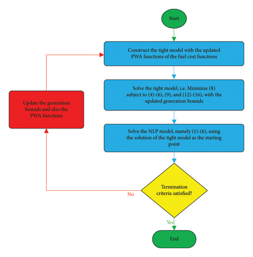
To achieve this, we solve a MILP model built with several segments. Next, we solve the ED model, referred to as (1)–(6), using a nonlinear programming (NLP) algorithm. We use the solution from the MILP model as the starting point for this algorithm. The NLP algorithm performs a local search to improve the solution. In the MINLP models (1)–(6), we set the binary variables related to fuel selection based on the solution obtained from the tight MILP model. This transforms the MINLP model into an NLP model. After solving the NLP model, we tighten the generation bounds around the NLP solution. Then, we create new PWA functions using new breakpoints that are evenly distributed within the tightened generation boundaries. Again, we solve the tight and the NLP models using these updated PWA functions. This process iteratively improves the PWA function accuracy near the optimal solutions. As a result, we can expect to generate a series of increasingly better solutions.

The flowchart of the iterative solution approach is summarized in the following and shown in Figure 1. The generation bounds are initially set as

. They are tightened quickly as the iterative method progresses. In the following steps, we use t to denote the iteration number.

1.
Distribute the breakpoints of the fuel cost functions evenly to construct their PWA functions based on the last generation bounds and then build the tight model.
2.
Solve the tight model.
3.
Solve the NLP model using the solution from the tight model as the starting point. We label the NLP solution as .
4.
Check if the termination criteria are met.
5.
Tighten the generation bounds around the NLP solution as follows:
()

()

()
where and . As shown, the generation bounds are tightened exponentially as 1/2^t, leading to fast convergence. The termination criterion is either the maximum number of iterations, which is set at five, or the following condition:
()
where O_t represents the objective function obtained in (1) during iteration t, namely, O_t = ∑_n∈NF_n.

Details are in the caption following the image — **Figure 1**
Open in figure viewer PowerPoint

Flowchart of the proposed iterative solution method.

4. Numerical Evaluation

This section uses eight case studies, including 10-unit, 20-unit, 40-unit, 80-unit, 160-unit, 320-unit, 640-unit, and 1280-unit, to test the proposed approach’s effectiveness. The case studies are created by modifying the number of units and load demands based on a 10-unit case [21]. All units in the case studies have the MF options and VLPs. Transmission losses are neglected in this analysis [22].

We have implemented the proposed approach in GAMS 24.1.3. The relative optimality gap in CPLEX 12.5.1.0, our solver, is set to 1e-3 to terminate the solution process at each iteration of the proposed approach. The maximum number of iterations in the iterative solution method is five. We used SQP within GAMS as the NLP solver with its default settings. We ran the simulations on a laptop with 2.7 GHz processors and 8 GB RAM.

tFirst, in Section 4.1, we validate the proposed approach using the eight case studies and compare our results with existing algorithms in the literature. Then, Section 4.2 analyzes the convergence characteristic of the solution method proposed. Subsequently, we compare the performance of the iterative solution method presented with a ST solution method in Section 4.3. Finally, Section 4.4 verifies the efficacy of the tight model against the standard formulation.

Due to space limitation, we provide generation dispatch results (unit generations in the optimal solution obtained) as “Supporting Information (available here).”

4.1. Validation of the Proposed Approach

In this section, we compare the proposed method with earlier nature-inspired techniques. Unlike the proposed method, nature-inspired algorithms solve the ED problem without transforming the formulation, as they do not rely on derivatives or convexity assumptions. However, because these algorithms use stochastic search strategies, they lack robustness and may produce different solutions in each run.

The nature-inspired methods can escape from local minimums since they carry out parallel searches using a group of candidate solutions rather than one point. However, they may face premature convergence or may fail to converge because they do not use standard mathematical techniques that are proven to ensure convergence. Furthermore, utilizing a group of solutions to solve a problem requires significant computational effort and results in longer solution times.

Thus, we evaluate the ED solution methods based on robustness, solution optimality, and computational time.

4.1.1. The 10-Unit Case Study

This case study has ten thermal generating units with the MF option and VLP, making a nonconvex MINLP problem. Thus, one can assess the proposed approach’s effectiveness in addressing the MINLP ED problem for this case study. Table 1 presents the solution found by the approach proposed and solutions from other optimization methods in the field. The table shows the results of the nature-inspired methods statistically as their best, mean, and worst solutions since they do not provide a unique solution across multiple runs. The global minimum is about 623.82 $/h. The proposed approach converges to 623.83 $/h, which is very close to the global minimum, indicating the validity of the tight model and solution method.

Table 1. The optimal solutions of optimization methods in the 10-unit case study.

Method	Best ($/h)	Mean ($/h)	Worst ($/h)
CGA_MU [23]	624.72	627.61	633.87
IGA_MU [23]	624.52	625.87	630.87
DE [24]	624.51	624.52	624.55
PSO [24]	624.51	624.51	624.51
IJAYA [8]	623.92	623.99	624.05
CLPSO [8]	623.92	624.00	624.05
TLBO [21]	623.88	623.94	623.97
CSA [26]	623.87	623.95	626.37
ORCSA [27]	623.86	623.90	623.94
DE [21]	623.85	623.88	623.89
RTLBO [8]	623.85	624.87	635.14
PPSO [8]	623.85	623.92	624.02
SaDE [21]	623.83	623.85	623.85
DE/BBO [21]	623.83	623.84	623.85
TLABC [8]	623.83	623.91	624.00
CCEDE [25]	623.83	623.86	623.89
BPSO [21]	623.83	623.84	623.87
JADE [21]	623.82	623.83	623.83
MIMO [21]	623.82	623.82	623.83
AGDE [8]	623.82	623.82	623.83
DPADE [21]	623.82	623.82	623.82
FV-ICLPSO [8]	623.82	623.82	623.82
Proposed	623.83	—	—

In [21], the competitive algorithms BPSO, TLBO, MIMO, DE, DE/BBO, SaDE, JADE, and DPADE identify the solution in 8.94, 10.07, 21.53, 9.01, 10.11, 9.97, 10.55, and 10.34 s, respectively. In contrast, the proposed approach identifies the same solution in just 0.84 s, demonstrating its efficiency. Since the employed hardware for the algorithms in [21] has not been reported, we cannot provide an exact comparison.

From Table 1, we see that most methods were able to explore the solution space of this small ED problem and provide high-quality solutions. However, the methods are not as robust as the approach proposed. In other words, nature-inspired methods typically offer a range of solutions in their applications rather than a single solution, as indicated by the mean or worst solutions in the table.

4.1.2. The 20-Unit Case Study

The second case is introduced by doubling the number of units and load of the 10-unit case study, measuring the performance of the approach proposed in a larger problem. Table 2 displays the results of the proposed approach alongside existing ED solution methods. As the table shows, the approach finds a more optimal solution than the existing methods, suggesting the effectiveness of the approach proposed.

Table 2. The optimal solutions of optimization methods in the 20-unit case study.

Method	Best ($/h)	Mean ($/h)	Worst ($/h)
IGA-MU [23]	1249.12	NA	NA
CSA [26]	1247.84	1248.00	1249.80
ED-DE [28]	1247.80	NA	NA
ORCSA [27]	1247.79	1247.79	1249.62
PGPSO [17]	1247.73	1248.96	1259.22
Proposed	1247.69	—	—

Abbreviation: NA, not available.

Table 2 shows that the competitive PGPSO algorithm may yield poor solutions; e.g., its worst result was 1259.22 $/h, the poorest among the methods listed.

In contrast, the proposed approach consistently identifies 1247.69 $/h as the optimal solution.

The PGPSO algorithm converges in 4.08 s using 2.1 GHz processors. In contrast, the proposed approach requires only 0.87 s to converge, illustrating its efficiency advantage.

4.1.3. The 40-Unit Case Study

This case study includes 40 thermal units that experience MF and VLP issues. The units with these issues create a nonlinear, nonconvex optimization problem with integer variables making it difficult to apply optimization methods. Table 3 summarizes the solutions obtained using various optimization algorithms, including the approach proposed. The table shows that the proposed method achieved the lowest cost of 2495.38 $/h, followed closely by the PGPSO, which is a competitive algorithm.

Table 3. The optimal solutions of optimization methods in the 40-unit case study.

Method	Best ($/h)	Mean ($/h)	Worst ($/h)
ORCSA [27]	2495.96	2496.63	2498.15
CSO [29]	2495.79	2496.63	2497.13
PGPSO [17]	2495.62	2499.61	2512.91
Proposed	2495.38	—	—

One advantage of the approach is that it consistently achieves the same optimal solution regardless of the initial points. In contrast, the results from the PGPSO and other nature-inspired algorithms in the table depend on their initial solutions (swarm), which can significantly alter the final outcomes.

In this case, the competitive algorithm PGPSO takes 18.65 s to find its solution (using 2.1 GHz processors). The proposed approach, however, finds a more optimal solution in just 0.99 s, demonstrating a significant computational advantage.

Therefore, the proposed approach can reliably identify the optimal solution for this case study, highlighting the effectiveness of the tight model and solution method.

4.1.4. The 80-Unit Case Study

The 80-unit case is created by repeating the 10-unit case study eight times. Due to the many units with nonconvex and discrete feasible sets, this case contains numerous local minima, complicating its solution. This validates the effectiveness of the tight model in representing the 80-unit MINLP solution space. Table 4 compares our solution with results from the existing literature on ED. The many optimization methods listed in the table show that several previous studies have used the 80-unit case to test their solution algorithms. The FV-ICLPSO, DPADE, and the presented approach have achieved the best performance among the optimization methods in the table.

Table 4. The optimal solutions of optimization methods in the 80-unit case study.

Method	Best ($/h)	Mean ($/h)	Worst ($/h)
CGA-MU [23]	5008.14	NA	NA
IGA-MU [23]	5003.88	NA	NA
TLBO [21]	5002.92	5011.81	5031.31
RTLBO [8]	4998.74	5011.44	5030.11
TLABC [8]	4998.70	5007.50	5027.59
CLPSO [8]	4995.92	4996.56	4997.07
IJAYA [8]	4995.58	5002.46	5029.87
DE [21]	4994.45	4994.76	4995.04
PGPSO [17]	4994.28	5003.03	5021.02
SSO [15]	4993.46	5002.91	5097.83
PPSO [8]	4993.28	5003.79	5017.34
ED-DE [28]	4992.71	NA	NA
CSA [26]	4992.69	4993.73	5003.43
ORCSA [27]	4992.42	4994.50	4995.67
SaDE [21]	4992.29	4992.50	4993.72
AGDE [8]	4992.23	4992.42	4992.57
MIMO [21]	4991.95	4996.44	5012.57
DE/BBO [21]	4991.53	4991.65	4991.83
BPSO [21]	4991.15	4991.51	4993.00
CSO [29]	4990.93	4991.29	4992.00
JADE [21]	4990.91	4990.95	4990.99
ISSO [15]	4990.87	4991.20	4993.87
DPADE [21]	4990.79	4990.81	4990.83
FV-ICLPSO [8]	4990.65	4990.69	4990.73
Proposed	4990.80	ED-DE [22]	4992.71

Abbreviation: NA, not available.

While the FV-ICLPSO and DPADE produced high-quality results in their best solutions, as shown in the second column of the table, their impressive performances cannot be assured since they rely on stochastic mechanisms that lack a strong mathematical backing.

Regarding computational efficiency, the proposed approach finds its optimal solution in 1.87 s using standard 2.7 GHz processors, whereas DPADE reaches a nearly identical optimal solution in 135.26 s. The hardware used for DPADE implementation is not reported in [21], so we can only provide an approximate comparison. However, since we used standard hardware, the significant difference in computational times suggests the superior efficiency of the proposed approach. Unfortunately, the computational time for FV-ICLPSO is not available in [8].

Overall, the quality of the solutions and the short solution time of the proposed approach confirm the effectiveness of the tight model and the strength of the iterative method.

4.1.5. The 160-Unit Case Study

One can build the 160-unit case study by doubling the 80-unit case. Owing to the complex multimodal nature of this problem, many earlier works have assessed their algorithms using the 160-unit case. Table 5 presents the results from these earlier works and the proposed method for solving this case study. The table illustrates that the proposed approach can reproduce the best optimal cost, around 9981 $/h, validating the effectiveness of the proposed iterative solution method and the tight model. Besides, the results illustrate that the solutions from nature-inspired algorithms often differ from their best outcomes. These deviations reveal their unreliable behavior in finding the optimal solution for the 160-unit case study. In contrast, the proposed approach consistently yields a unique minimum.

Table 5. The optimal solutions of optimization methods in the 160-unit case study.

Method	Best ($/h)	Mean ($/h)	Worst ($/h)
CGA-MU [23]	10,143.73	NA	NA
IGA-MU [23]	10,042.47	NA	NA
PSO [30]	10,036.20	NA	NA
HPSO-DE [30]	10,013.01	NA	NA
ED-DE [28]	10,012.68	NA	NA
FBHPSO-DE [30]	10,011.07	NA	NA
RCCRO [32]	10,009.52	10,009.52	10,009.58
BBO [33]	10,008.71	10,009.16	10,010.59
RTLBO [8]	10,008.38	10,023.08	10,039.73
DE/BBO [33]	10,007.05	10,007.56	10,010.26
TLABC [8]	10,006.51	10,029.81	10,050.62
PGPSO [17]	10,004.73	10,032.49	10,107.17
ORCCRO [33]	10,004.20	10,004.21	10,004.45
TLBO [21]	10,003.04	10,025.24	10,047.14
QBA [13]	10,001.99	10,002.88	10,004.98
CLPSO [8]	9996.95	9999.07	10,000.41
GQBA [13]	9996.14	9997.29	9999.12
IJAYA [8]	9996.10	10,011.94	10,031.00
PI-CBA [35]	9995.81	10,029.08	10,069.74
CGQBA [13]	9994.32	9998.23	10,026.00
PPSO [8]	9993.91	10,016.91	10,040.60
DE [21]	9990.76	9992.22	10,001.69
CSA [26]	9990.65	9996.64	10,014.02
ORCSA [27]	9989.94	9992.05	9996.83
DWPSO [31]	9988.75	9993.68	9999.31
AGDE [8]	9987.43	9988.20	9997.42
EPSDE [21]	9986.86	9987.59	9996.42
SaDE [21]	9986.80	9988.31	9999.54
BPSO [21]	9986.41	9988.64	9990.65
DE/BBO [21]	9985.98	9986.69	9987.47
CSO [29]	9984.24	9984.92	9986.36
MIMO [21]	9983.78	9998.78	10,017.76
JADE [21]	9983.25	9986.78	10,004.13
DPADE [21]	9982.56	9982.68	9982.86
FV-ICLPSO [8]	9981.59	9981.78	9981.92
MSOS [34]	9981.31	9981.98	9983.64
Proposed	9981.52	—	—

Abbreviation: NA, not available.

We can identify three algorithms—MSOS, FV-ICLPSO, and the proposed method—as the top performers among the techniques listed in Table 5 because they achieve the minimum cost of $9981 per hour. The MSOS algorithm reaches the optimal solution in 25.72 s, using a 2.2 GHz CPU, which has processing power similar to our 2.7 GHz processors. However, the proposed method finds the optimal solution of $9981 per hour in only 3.2 s, making it about eight times faster than the MSOS. As noted earlier, the computational time for FV-ICLPSO is not reported in [8], so we cannot assess its efficiency.

4.1.6. The 320-Unit Case Study

This case is constructed by repeating the 10-unit case 32 times, resulting in a significantly larger and more complex solution space compared with the 10-unit case. The complex solution space allows for a thorough evaluation of the effectiveness and efficiency of the proposed method for solving the case study. Table 6 displays the solutions from the proposed approach and existing algorithms in the area, sourced from relevant works. The table shows that the proposed approach solves the ED problem effectively, returning a high-quality optimal cost of 19,962.76 $/h. The table also shows that only MSOS, ISSO, and FV-ICLPSO algorithms can compete with the proposed approach in finding high-quality solutions. However, the third and fourth columns of the table demonstrate that these algorithms usually offer inconsistent solutions, making them inappropriate for practical applications.

Table 6. The optimal solutions of optimization methods in the 320-unit case study.

Method	Best ($/h)	Mean ($/h)	Worst ($/h)
SSSO [15]	20,294.16	20,962.64	21,482.06
TLBO [21]	20,060.56	20,082.25	20,111.99
BPSO [21]	20,027.11	20,047.44	20,080.94
MIMO [21]	20,018.61	20,045.56	20,100.77
PPSO [8]	20,014.82	20,040.01	20,071.14
TLABC [8]	20,014.70	20,043.88	20,069.29
RTLBO [8]	20,011.93	20,031.93	20,077.79
DE/BBO [21]	19,997.66	20,003.64	20,008.77
CLPSO [8]	19,992.44	19,994.84	19,996.91
IJAYA [8]	19,991.09	19,994.03	20,000.75
DE [21]	19,985.55	19,992.86	20,010.46
SaDE [21]	19,980.32	19,983.55	19,989.28
AGDE [8]	19,978.77	19,980.51	19,988.64
JADE [21]	19,975.51	19,983.75	20,011.59
CSO [29]	19,969.94	19,972.25	19,974.99
DPADE [21]	19,969.42	19,972.82	19,983.23
OPIO [14]	19,968.95	19,972.16	19,978.91
FV-ICLPSO [8]	19,963.23	19,963.48	19,963.71
ISSO [15]	19,963.14	19,964.46	19,989.38
MSOS [34]	19,962.62	19,963.71	19,965.25
Proposed	19,962.76	—	—

Regarding efficiency, the proposed approach finds the optimal solution for this ED problem in about 7 s. The MSOS (with 2.2 GHZ CPUs) and ISOS (with 2.4 GHZ CPUs) solve the problem in 96.41 and 6.4 s, suggesting the proposed approach and MSOS are more efficient than the ISOS algorithm.

Therefore, in the 320-unit case, the proposed approach quickly identifies a solution of high quality without deviations. Accordingly, the approach can maintain its capability in larger case studies.

4.1.7. The 640-Unit Case Study

One can double the 320-unit case to obtain the larger 640-unit case study, which has a more complex feasible space. The 640-unit case, which includes many indicator variables, tests the effectiveness of the proposed approach in solving a large and nonconvex ED problem. Table 7 compares the solution from the proposed approach with previous algorithms in the field. As the table shows, the FV-ICLPSO has found the best optimal solution thus far, yielding 39,930 $/h. Nonetheless, the proposed approach improves on this by achieving an optimal cost of 39,925.77 $/h. Therefore, increasing the size and complexity of the case studies highlights the potential advantages of the approach proposed.

Table 7. The optimal solutions of optimization methods in the 640-unit case study.

Method	Best ($/h)	Mean ($/h)	Worst ($/h)
BPSO [21]	40,578.44	40,668.65	40,766.11
MIMO [21]	40,323.27	40,381.63	40,489.60
DE/BBO [21]	40,214.76	40,250.05	40,289.80
TLBO [21]	40,185.26	40,239.28	40,276.33
PPSO [8]	40,112.33	40,152.01	40,237.97
RTLBO [8]	40,075.64	40,125.13	40,205.86
TLABC [8]	40,069.46	40,153.46	40,212.02
CLPSO [8]	40,017.13	40,022.24	40,027.84
DE [21]	40,008.43	40,034.90	40,067.47
IJAYA [8]	40,007.84	40,019.66	40,041.37
JADE [21]	39,981.33	39,998.00	40,049.76
SaDE [21]	39,980.74	39,991.92	40,026.41
AGDE [8]	39,970.16	39,974.20	39,990.56
CSO [29]	39,964.06	39,968.03	39,974.19
DPADE [21]	39,963.96	39,987.00	40,025.30
OPIO [14]	39,963.78	39,964.75	39,967.82
CSS [36]	39,960.71	39,998.58	40,064.11
LFA [37]	39,957.77	39,969.29	39,974.66
ACSS [36]	39,950.79	39,977.32	40,018.46
FV-ICLPSO [8]	39,930.00	39,930.92	39,938.99
Proposed	39,925.77	—	—

Furthermore, the results in the table show that the deviations of the nature-inspired algorithms have increased in this larger case study compared with the earlier cases. For example, we can observe a 188 $/h difference between the best and worst solution of the BPSO algorithm in the 640-unit case. In contrast, the results in Table 6 show only a 0.5 $/h difference between the best and worst solutions of the FV-ICLPSO algorithm in the 320-unit case. However, in the 640-unit case study shown in Table 7, the difference is 9 $/h for the same algorithm. On the other hand, the proposed approach can guarantee convergence to the unique solution of 39,925.77 $/h without concerns about solution deviations, validating its robustness.

4.1.8. The 1280-Unit Case Study

This case study has 1280 generating units with the MF and VLP. To the best of our knowledge, the case is the largest ED case study with the MF and VLP in the literature. This case builds a large, nonconvex, and discrete solution space with many continuous and integer decision variables. Besides, it contains many local minimums owing to its nonconvex structure. Accordingly, it can question the efficiency of the tight model and the proposed solution method. Table 8 shows the solutions obtained by the approach proposed and those of other algorithms in the area.

Table 8. The optimal solutions of optimization methods in the 1280-unit case study.

Method	Best ($/h)	Mean ($/h)	Worst ($/h)
BPSO [21]	83,098.1	83,299.97	83,498.41
MIMO [21]	82,517.83	82,869	83,166.66
DE/BBO [21]	81,373.55	81,532.49	81,688.18
TLBO [21]	80,619.4	80,729.03	80,871.75
DE [21]	80,480.98	80,542.61	80,636.7
JADE [21]	80,090.83	80,137.91	80,188.44
SaDE [21]	80,063.34	80,105.03	80,151.86
DPADE [21]	80,044.65	80,145.53	80,767.5
Proposed	79,851.73	—	—

The table demonstrates that the proposed approach outperforms other algorithms in terms of solution quality. Table 8 illustrates that the minimum cost found by the earlier algorithms, specifically the DPADE algorithm, is 80,044.65 $/h [21]. Our approach achieves an optimal cost of 79,851.73 $/h, enhancing the best solution in this case study.

Regarding robustness, the results show that the DPADE algorithm converges to 80,767.5 $/h in its worst performance among 30 trial runs [21]. Furthermore, it may converge to higher with an increased number of trial runs. The BPSO, another competitive algorithm in the table, offers a worst solution of 83,498.41 $/h, suggesting it may perform poorly in its trial runs. In contrast, the approach proposed constantly converges to its optimal cost of 79,851.73 $/h, illustrating its robustness in solving the ED problem.

From a computational time viewpoint, while the proposed approach reaches 79,851.73 $/h in 76.4 s, the DPADE algorithm converges to 80,044.65 $/h in 5082.4 s. The significant difference in the computational times demonstrates the advantage of the approach in terms of efficiency. However, we cannot accurately compare the efficiency of the two methods, as the DPADE does not specify the hardware used [21].

The solution quality and the computational time of the proposed approach verify that it can efficiently solve large-scale MINLP ED problems and identify high-quality solutions.

4.2. Convergence Characteristics of the Proposed Approach

Figures 2(a), 2(b), 2(c), 2(d), 2(e), 2(f), 2(g), and 2(h) display the convergence characteristics of the approach proposed in the considered case studies. The figures show that the approach yields solutions of high quality in the first iteration. These results imply that the proposed models can accurately mimic the solution space of ED. In addition, the figures reveal that the second iteration achieves greater cost improvements than the later iterations.

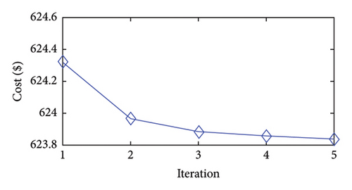
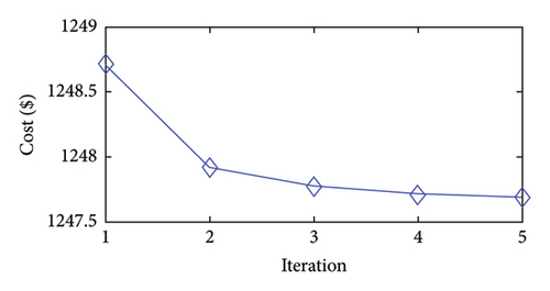
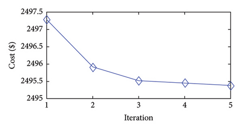
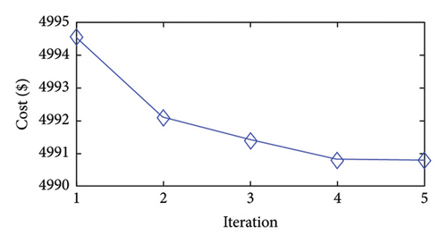
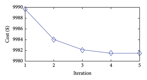
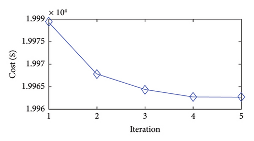
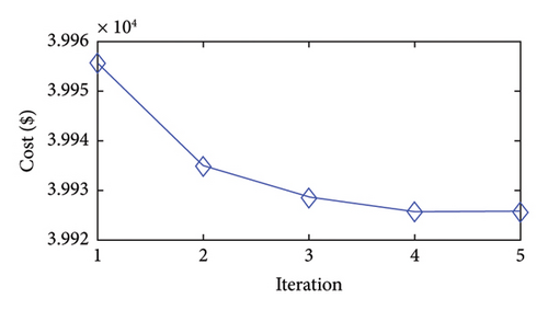
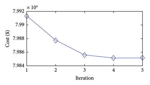
Moreover, the proposed approach effectively reaches its final solution by the fourth iteration. After this point, the changes in the objective function become minimal, and the stopping criteria are met. Specifically, in the fourth iteration, the bounds on the generation variables decrease to (1/2)³ of their initial values. For instance, the initial generation range of 80 MW for a unit is reduced to 10 MW in the fourth iteration. The feasible bound shrinks exponentially during iterations of the approach presented. Accordingly, in the later iterations, the existing nonlinear functions may behave more linearly within the narrower bounds, facilitating convergence to the optimal solutions of the problem.

In summary, the approach explores the whole solution space and identifies the approximate region of the global minimum in the first iteration. Then, in the subsequent iterations, the approach focuses on this region to obtain a more precise minimum solution through the bound-tightening technique and updated PWA functions.

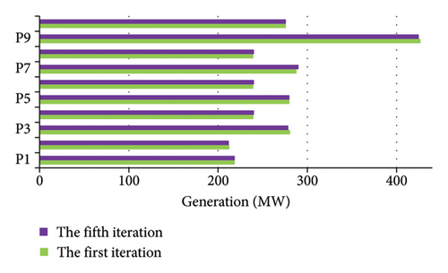
As an illustration, Figure 3 compares the unit generations in the first iteration with those in the fifth (final) iteration for the 10-unit case study. It shows that the changes in the unit generations are minimal after the first iteration.

4.3. Comparison of the Proposed Iterative Solution Method With a ST Method

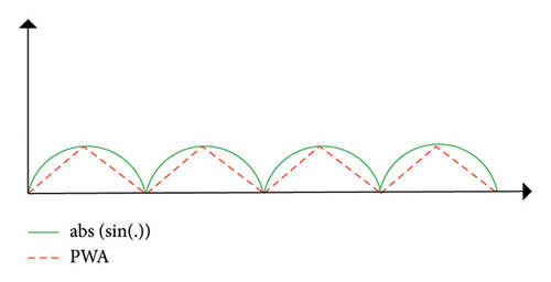
Instead of using the proposed iterative solution method, one can use a ST technique to solve the ED problem. In the ST, we need to build a PWA function that mimics the ED nonlinear functions more precisely, as it lacks another stage to improve its approximation. Therefore, the ST method must use significantly more segments than the proposed iterative method. Figure 4 illustrates the nonlinear term abs (sin(·)), which appears in the cost function (3) and its PWA function. As the figure illustrates, the ST method requires at least two segments for each period of the abs (sin(·)) function to closely approximate it.

To improve accuracy, we constructed a more precise PWA function by using two segments for each of its periods. We then applied this PWA function to solve the ED problem in a single stage. In other words, we followed the process shown in Figure 1 just once. Table 9 summarizes the costs obtained from the iterative solution and the ST methods. The results in the table show that the ST only slightly improves the solution quality in Cases 1–4. Since the ST uses more segments than the iterative method, it can better represent the problem’s feasible space and obtain relatively better solutions.

Table 9. Comparison of the proposed iterative method with the single-stage (ST) technique.

Case study	Cost ($/h)		Computational time (S)
Case study	Proposed	ST	Proposed	ST
10-unit	623.838	623.827	0.84	10.61
20-unit	1247.690	1247.653	0.87	37.62
40-unit	2495.375	2495.306	0.99	110.17
80-unit	4990.803	4990.612	1.87	391.72
160-unit	9981.519	OM^a	3.24	—
320-unit	19,962.760	OM^a	7.06	—
640-unit	39,925.770	OM^a	20.10	—
1280-unit	79,851.730	OM^a	76.34	—

^aOM: out of memory.

Nevertheless, the ST is computationally expensive. For example, it requires 10.61 s to solve the 10-unit case, which is 12 times slower than the proposed iterative method, which takes only 0.84 s. We see the computational advantage of the iterative method in larger cases. For instance, in the 80-unit case study, the proposed method converges 391.72/1.87≅210 times faster than the ST.

Furthermore, the ST cannot solve the ED cases larger than the 80-unit case because it employs too many segments, which should be modeled using integer variables and combinatorial constraints. As a result, the ST method requires a large amount of memory. Thus, the ST requires extreme memory allocation. Consequently, in larger cases, the software cannot allocate enough memory to model the ED using the ST technique and returns no solution. In contrast, the iterative method utilizes only three segments to represent the nonlinear function, requiring fewer system resources to solve the problem. It focuses on gradually improving the approximation near the candidate solutions rather than trying to derive an exact representation for the whole function domain right from the beginning of the solution process.

4.4. Evaluation of Computational Time

In this section, we will first compare the tight formulation, specifically (4)–(6), (9), and (12)–(16) with the standard formulation presented in (4)–(6) and (9)–(15) by analyzing their computational times. Then, we will compare the proposed method with nature-inspired algorithm.

Table 10 shows the computational times for the two formulation techniques across the eight cases considered. The last column in the table shows the speedup obtained by the tight formulation compared to the standard formulation.

Table 10. Comparison of the tight and standard formulations in terms of computational times.

Case study	Computational times
Case study	Standard formulation	Tight formulation	Speedup (%)
10-unit	1.03	0.84	18.49
20-unit	1.11	0.87	22.07
40-unit	1.28	0.99	22.70
80-unit	2.30	1.87	18.52
160-unit	4.10	3.24	21.05
320-unit	10.28	7.06	31.34
640-unit	35.87	20.10	43.98
1280-unit	139.32	76.34	45.21

A comparison of the second and third columns of the table illustrates that the tight formulation converges considerably faster than the standard model. The last column reveals that the tight formulation can reduce the solution time by 18%–45% in the case studies analyzed. In particular, the speedup in the solution process tends to improve as the size of the ED problem increases, highlighting the efficiency of the tight formulation for larger case studies.

Figure 5 illustrates the contribution of each iteration to the computational times of the tight and standard formulations in the 1280-unit case study. First, the computational times for iterations show a descending trend because of the bound-tightening technique. Second, the computational times for all iterations in the tight formulation are less than those in the standard formulation on account of the local ideality of the tight model. In particular, during the first iteration, the tight formulation converges in 18 s, which is much faster than the standard formulation, which takes 67.5 s.

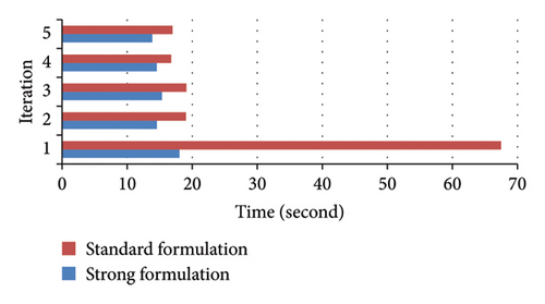
Table 11 compares the computational times of the proposed method with those of nature-inspired algorithms. The proposed method outperforms the earlier methods in computational time, as shown in the table. Larger case studies further highlight the advantages of the proposed method.

Table 11. Comparison of the computational times of solution methods.

Method	Time (s)	CPU (GHz)
10-Unit case study
MIMO [21]	21.53	NA
JADE [21]	10.55	NA
DPADE [21]	10.34	NA
DE/BBO [21]	10.11	NA
TLBO [21]	10.07	NA
SaDE [21]	9.97	NA
DE [21]	9.01	NA
BPSO [21]	8.94	NA
Proposed	0.84	2.7

20-unit case study
PGPSO [17]	4.08	2.1
Proposed	0.87	2.7

40-unit case study
PGPSO [17]	18.65	2.1
Proposed	0.99	2.7

80-unit case study
BPSO [21]	131.6	NA
TLBO [21]	128.78	NA
MIMO [21]	183.44	NA
DE [21]	126.83	NA
DE/BBO [21]	160.47	NA
SaDE [21]	138.1	NA
JADE [21]	134.8	NA
DPADE [21]	135.26	NA
Proposed [21]	1.87	2.7

160-unit case study
MIMO [21]	300.9	NA
DE/BBO [21]	290.92	NA
EPSDE [21]	246.51	NA
JADE [21]	244.94	NA
DPADE [21]	241.72	NA
SaDE [21]	241.28	NA
DE [21]	237.21	NA
TLBO [21]	235.16	NA
BPSO [21]	219.56	NA
MSOS [34]	25.72	2.2
Proposed	3.24	2.7

320-unit case study
DE/BBO [21]	592.25	NA
MIMO [21]	571.65	NA
JADE [21]	506.78	NA
SaDE [21]	485.57	NA
DE [21]	484.82	NA
DPADE [21]	481.3	NA
TLBO [21]	471.27	NA
BPSO [21]	458.02	NA
MSOS [34]	96.41	2.2
ISOS [15]	6.40	2.4
Proposed	7.06	2.7

640-unit case study
DE/BBO [21]	1709.93	NA
MIMO [21]	1673.12	NA
TLBO [21]	1598.29	NA
SaDE [21]	1552.39	NA
DPADE [21]	1542.91	NA
JADE [21]	1535.41	NA
BPSO [21]	1502.98	NA
DE [21]	1494.73	NA
Proposed	20.1	2.7

1280-unit case study
MIMO [21]	5477.9	NA
JADE [21]	5243.46	NA
DE/BBO [21]	5194.05	NA
BPSO [21]	5183.51	NA
SaDE [21]	5085.75	NA
DPADE [21]	5082.41	NA
DE [21]	5002.19	NA
TLBO [21]	4689.68	NA
Proposed	76.34	2.7

As seen, the proposed method converges more than 10 times faster than the BPSO, which is the fastest algorithm in previous studies for the 10-unit case study. However, in the 1280-unit case study, the proposed method converges more than 61 times faster than the TLBO, which is also one of the fastest algorithms in earlier studies.

The hardware used in some earlier studies has not been reported in their associated papers. Nonetheless, since we employed commodity hardware, the considerable difference in computational times may show the superior efficiency of our proposed approach. The superiority can be attributed to the tightness of the proposed model and the effectiveness of mixed-integer solvers.

In our future work, we plan to improve our method to handle multiarea ED [38] and combined heat-and-power ED [39].

5. Conclusion

This paper proposes a tight formulation and an iterative solution method to address the MF option and complex cost functions, rendering the ED a nondifferentiable, nonconvex MINLP problem. The numerical evaluations conducted on the eight case studies illustrate the following:

1.
The proposed approach solves the complex MINLP ED effectively and manages the dispatch of thermal power plants. It provides high-quality solutions in reasonable computational times without any deviations. This approach provides results similar to the best existing algorithms or obtains even more optimal solution in the case studies adopted.
2.
As for the computational times, the proposed approach finds its optimal solution faster than the competitive algorithms, especially in the large case studies considered.
3.
The proposed iterative solution derives a high-quality solution in the first iteration and gradually improves it in next iterations using the bound-tightening technique and updated PWA functions.
4.
The proposed iterative method is significantly more efficient than the ST technique, particularly in large case studies. In addition, the ST technique cannot solve case studies larger than the 80-unit case due to memory allocation issues.
5.
The proposed tight model is more efficient than the standard formulation. Specifically, it speeds up the solution process by 18%–45% in the case studies.

Conflicts of Interest

The author declares no conflicts of interest.

Funding

This research received no specific grant from any funding agency in the public, commercial, or not-for-profit sectors.

Supporting Information

Supporting files contain the generation dispatch results from the proposed method’s optimal solution.

Open Research

Data Availability Statement

Data for the test systems used in this study are available in the referenced publications.

Supporting Information

References

1 Miracle D. B., Viral R., Tiwari P., and Bansal M., Hybrid Metaheuristic Model for Optimal Economic Load Dispatch in Renewable Hybrid Energy System, International Transactions on Electrical Energy Systems. (2023) 2023, 1–25, https://doi.org/10.1155/2023/5395658.
10.1155/2023/5395658
Google Scholar
2 Grossmann I. E., Advanced Optimization for Process Systems Engineering, 2021, Cambridge University Press.
10.1017/9781108917834
Google Scholar
3 Franzoi R. E., Menezes B. C., Kelly J. D., Gut J. A., and Grossmann I. E., Large-Scale Optimization of Nonconvex MINLP Refinery Scheduling, Computers & Chemical Engineering. (2024) 186, https://doi.org/10.1016/j.compchemeng.2024.108678.
10.1016/j.compchemeng.2024.108678
Google Scholar
4 Ovalle D., Liñán D. A., Lee A. et al., Logic-Based Discrete-Steepest Descent: A Solution Method for Process Synthesis Generalized Disjunctive Programs, 2024.
Google Scholar
5 Perez H. D., Joshi S., and Grossmann I. E., DisjunctiveProgramming. Jl: Generalized Disjunctive Programming Models and Algorithms for JuMP, 2023.
Google Scholar
6 D’Ambrosio C., Frangioni A., and Gentile C., Strengthening the Sequential Convex MINLP Technique by Perspective Reformulations, Optimization Letters. (2019) 13, no. 4, 673–684, https://doi.org/10.1007/s11590-018-1360-9, 2-s2.0-85057200958.
10.1007/s11590-018-1360-9
Google Scholar
7 Sharifzadeh H., An Extended Incremental Technique for Solving Economic Dispatch with Practical Considerations, Electric Power Systems Research. (2024) 233, https://doi.org/10.1016/j.epsr.2024.110455.
10.1016/j.epsr.2024.110455
Google Scholar
8 Xu S., Xiong G., Mohamed A. W., and Bouchekara H. R., Forgetting Velocity Based Improved Comprehensive Learning Particle Swarm Optimization for Non-Convex Economic Dispatch Problems With Valve-Point Effects and Multi-Fuel Options, Energy. (2022) 256, https://doi.org/10.1016/j.energy.2022.124511.
10.1016/j.energy.2022.124511
Google Scholar
9 Karimi N. and Khandani K., Social Optimization Algorithm With Application to Economic Dispatch Problem, International Transactions on Electrical Energy Systems. (2020) 30, no. 11, https://doi.org/10.1002/2050-7038.12593.
10.1002/2050-7038.12593
Google Scholar
10 V Ponnuvel S., Murugesan S., and P Duraisamy S., Multi-Objective Squirrel Search Algorithm to Solve Economic Environmental Power Dispatch Problems, International Transactions on Electrical Energy Systems. (2020) 30, no. 12, https://doi.org/10.1002/2050-7038.12635.
10.1002/2050-7038.12635
Google Scholar
11 Basu S., Kumar S., and Basu M., Horse Herd Optimization Algorithm for Economic Dispatch Problems, Engineering Optimization. (2023) 55, no. 5, 806–822, https://doi.org/10.1080/0305215x.2022.2035378.
10.1080/0305215X.2022.2035378
Google Scholar
12 Jeddi B. and Vahidinasab V., A Modified Harmony Search Method for Environmental/Economic Load Dispatch of Real-World Power Systems, Energy Conversion and Management. (2014) 78, 661–675, https://doi.org/10.1016/j.enconman.2013.11.027, 2-s2.0-84890849510.
10.1016/j.enconman.2013.11.027
Web of Science® Google Scholar
13 Rugema F. X., Yan G., Mugemanyi S., Jia Q., Zhang S., and Bananeza C., A Cauchy-Gaussian Quantum-Behaved Bat Algorithm Applied to Solve the Economic Load Dispatch Problem, IEEE Access. (2021) 9, 3207–3228, https://doi.org/10.1109/access.2020.3034730.
10.1109/ACCESS.2020.3034730
Web of Science® Google Scholar
14 Ramalingam R., Karunanidy D., Alshamrani S. S., Rashid M., Mathumohan S., and Dumka A., Oppositional Pigeon-Inspired Optimizer for Solving the Non-Convex Economic Load Dispatch Problem in Power Systems, Mathematics. (2022) 10, no. 18, https://doi.org/10.3390/math10183315.
10.3390/math10183315
Google Scholar
15 Kien L. C., Nguyen T. T., Hien C. T., and Duong M. Q., A Novel Social Spider Optimization Algorithm for Large-Scale Economic Load Dispatch Problem, Energies. (2019) 12, no. 6, https://doi.org/10.3390/en12061075, 2-s2.0-85063719735.
10.3390/en12061075
Google Scholar
16 Iqbal M. N., Bhatti A. R., Butt A. D., Sheikh Y. A., Paracha K. N., and Ashique R. H., Solution of Economic Dispatch Problem Using Hybrid Multi-Verse Optimizer, Electric Power Systems Research. (2022) 208, https://doi.org/10.1016/j.epsr.2022.107912.
10.1016/j.epsr.2022.107912
Google Scholar
17 Dieu V. N., Schegner P., and Ongsakul W., Pseudo-Gradient Based Particle Swarm Optimization Method for Non-Convex Economic Dispatch, Power, Control and Optimization. (2013) Springer.
10.1007/978-3-319-00206-4_1
Google Scholar
18 Sharifzadeh H., Two Efficient Logarithmic Formulations to Solve Nonconvex Economic Dispatch, Electric Power Systems Research. (2024) 229, https://doi.org/10.1016/j.epsr.2024.110123.
10.1016/j.epsr.2024.110123
Google Scholar
19 Sharifzadeh H., Sharp Formulations of Nonconvex Piecewise Linear Functions to Solve the Economic Dispatch Problem With Valve-Point Effects, International Journal of Electrical Power & Energy Systems. (2021) 127, https://doi.org/10.1016/j.ijepes.2020.106603.
10.1016/j.ijepes.2020.106603
Google Scholar
20 Sridhar S., Linderoth J., and Luedtke J., Locally Ideal Formulations for Piecewise Linear Functions With Indicator Variables, Operations Research Letters. (2013) 41, no. 6, 627–632, https://doi.org/10.1016/j.orl.2013.08.010, 2-s2.0-84884265006.
10.1016/j.orl.2013.08.010
Web of Science® Google Scholar
21 Chen X., Novel Dual-Population Adaptive Differential Evolution Algorithm for Large-Scale Multi-Fuel Economic Dispatch With Valve-Point Effects, Energy. (2020) 203, https://doi.org/10.1016/j.energy.2020.117874.
10.1016/j.energy.2020.117874
PubMed Google Scholar
22 Sharifzadeh H., An Enhanced McCormick Envelopes to Represent Kron’s Loss Formula, International Journal of Engineering. (2023) 36, no. 3, 585–593, https://doi.org/10.5829/ije.2023.36.03c.19.
10.5829/IJE.2023.36.03C.19
Google Scholar
23 Chiang C.-L., Improved Genetic Algorithm for Power Economic Dispatch of Units With Valve-Point Effects and Multiple Fuels, IEEE Transactions on Power Systems. (2005) 20, no. 4, 1690–1699, https://doi.org/10.1109/tpwrs.2005.857924, 2-s2.0-28244499291.
10.1109/TPWRS.2005.857924
Web of Science® Google Scholar
24 Manoharan P., Kannan P., Baskar S., and Iruthayarajan M., Penalty Parameter-Less Constraint Handling Scheme Based Evolutionary Algorithm Solutions to Economic Dispatch, IET Generation, Transmission & Distribution. (2008) 2, no. 4, 478–490, https://doi.org/10.1049/iet-gtd:20070423, 2-s2.0-44349149839.
10.1049/iet-gtd:20070423
Web of Science® Google Scholar
25 Ghasemi M., Taghizadeh M., Ghavidel S., and Abbasian A., Colonial Competitive Differential Evolution: An Experimental Study for Optimal Economic Load Dispatch, Applied Soft Computing. (2016) 40, 342–363, https://doi.org/10.1016/j.asoc.2015.11.033, 2-s2.0-84950259758.
10.1016/j.asoc.2015.11.033
Web of Science® Google Scholar
26 Vo D. N., Schegner P., and Ongsakul W., Cuckoo Search Algorithm for Non-Convex Economic Dispatch, IET Generation, Transmission & Distribution. (2013) 7, no. 6, 645–654, https://doi.org/10.1049/iet-gtd.2012.0142, 2-s2.0-84880682225.
10.1049/iet-gtd.2012.0142
Web of Science® Google Scholar
27 Nguyen T. T. and Vo D. N., The Application of One Rank Cuckoo Search Algorithm for Solving Economic Load Dispatch Problems, Applied Soft Computing. (2015) 37, 763–773, https://doi.org/10.1016/j.asoc.2015.09.010, 2-s2.0-84942745316.
10.1016/j.asoc.2015.09.010
Web of Science® Google Scholar
28 Wang Y., Li B., and Weise T., Estimation of Distribution and Differential Evolution Cooperation for Large Scale Economic Load Dispatch Optimization of Power Systems, Information Sciences. (2010) 180, no. 12, 2405–2420, https://doi.org/10.1016/j.ins.2010.02.015, 2-s2.0-77950298367.
10.1016/j.ins.2010.02.015
Web of Science® Google Scholar
29 Meng A., Li J., and Yin H., An Efficient Crisscross Optimization Solution to Large-Scale Non-Convex Economic Load Dispatch With Multiple Fuel Types and Valve-Point Effects, Energy. (2016) 113, 1147–1161, https://doi.org/10.1016/j.energy.2016.07.138, 2-s2.0-84982731498.
10.1016/j.energy.2016.07.138
Web of Science® Google Scholar
30 Naderi E., Azizivahed A., Narimani H., Fathi M., and Narimani M. R., A Comprehensive Study of Practical Economic Dispatch Problems by a New Hybrid Evolutionary Algorithm, Applied Soft Computing. (2017) 61, 1186–1206, https://doi.org/10.1016/j.asoc.2017.06.041, 2-s2.0-85024833127.
10.1016/j.asoc.2017.06.041
Web of Science® Google Scholar
31 Kheshti M., Ding L., Ma S., and Zhao B., Double Weighted Particle Swarm Optimization to Non-Convex Wind Penetrated Emission/Economic Dispatch and Multiple Fuel Option Systems, Renewable Energy. (2018) 125, 1021–1037, https://doi.org/10.1016/j.renene.2018.03.024, 2-s2.0-85046016786.
10.1016/j.renene.2018.03.024
Web of Science® Google Scholar
32 Bhattacharjee K., Bhattacharya A., and Halder nee Dey S., Chemical Reaction Optimisation for Different Economic Dispatch Problems, IET Generation, Transmission & Distribution. (2014) 8, no. 3, 530–541, https://doi.org/10.1049/iet-gtd.2013.0122, 2-s2.0-84896853243.
10.1049/iet-gtd.2013.0122
Web of Science® Google Scholar
33 Bhattacharjee K., Bhattacharya A., and nee Dey S. H., Oppositional Real Coded Chemical Reaction Based Optimization to Solve Short-Term Hydrothermal Scheduling Problems, International Journal of Electrical Power & Energy Systems. (2014) 63, 145–157.
10.1016/j.ijepes.2014.05.065
Web of Science® Google Scholar
34 Secui D. C., A Modified Symbiotic Organisms Search Algorithm for Large Scale Economic Dispatch Problem With Valve-Point Effects, Energy. (2016) 113, 366–384, https://doi.org/10.1016/j.energy.2016.07.056, 2-s2.0-84978657904.
10.1016/j.energy.2016.07.056
Web of Science® Google Scholar
35 Shukla A. and Singh S. N., Pseudo-Inspired CBA for ED of Units With Valve-Point Loading Effects and Multi-Fuel Options, IET Generation, Transmission & Distribution. (2017) 11, no. 4, 1039–1045, https://doi.org/10.1049/iet-gtd.2016.1360, 2-s2.0-85015222471.
10.1049/iet-gtd.2016.1360
Web of Science® Google Scholar
36 Zakian P. and Kaveh A., Economic Dispatch of Power Systems Using an Adaptive Charged System Search Algorithm, Applied Soft Computing. (2018) 73, 607–622, https://doi.org/10.1016/j.asoc.2018.09.008, 2-s2.0-85053826729.
10.1016/j.asoc.2018.09.008
Web of Science® Google Scholar
37 Kheshti M., Kang X., Bie Z., Jiao Z., and Wang X., An Effective Lightning Flash Algorithm Solution to Large Scale Non-Convex Economic Dispatch With Valve-Point and Multiple Fuel Options on Generation Units, Energy. (2017) 129, 1–15, https://doi.org/10.1016/j.energy.2017.04.081, 2-s2.0-85018504741.
10.1016/j.energy.2017.04.081
Web of Science® Google Scholar
38 Sharifzadeh H., A Reliable Deterministic Method for Multi-Area Economic Dispatch Considering Power Losses, Energy Reports. (2024) 12, 2720–2731, https://doi.org/10.1016/j.egyr.2024.08.043.
10.1016/j.egyr.2024.08.043
Google Scholar
39 Hasanabadi R. and Sharifzadeh H., Solving Combined Heat and Power Economic Dispatch Using a Mixed Integer Model, Journal of Cleaner Production. (2024) 444, https://doi.org/10.1016/j.jclepro.2024.141160.
10.1016/j.jclepro.2024.141160
Google Scholar

All articles

Handling Multiple-Fuel Options in Economic Dispatch of Thermal Power Plants Through a Tight Model Applying Indicator Variables

Abstract

1. Introduction

2. Problem Statement