International Journal of Energy Research

Volume 2025, Issue 1 9924459

Research Article

Open Access

Reinforcement Learning-Based Injection Schedules for CO₂ Geological Storage Under Operation Constraints

Suryeom Jo

orcid.org/0000-0002-4449-4415

Mineral Exploration and Mining Research Center , Mineral Resources Division , Korea Institute of Geoscience and Mineral Resources , Daejeon , 34132 , Republic of Korea , kigam.re.kr

Search for more papers by this author

Tea-Woo Kim,

Tea-Woo Kim

orcid.org/0000-0001-8438-7318

CO₂ Geological Storage Research Center , Climate Change Response Division , Korea Institute of Geoscience and Mineral Resources , Daejeon , 34132 , Republic of Korea , kigam.re.kr

Search for more papers by this author

Changhyup Park,

Corresponding Author

Changhyup Park

[email protected]

orcid.org/0000-0001-8083-6809

Department of Energy and Resources Engineering , Kangwon National University , Chuncheon, Kangwon , 24341 , Republic of Korea , kangwon.ac.kr

Search for more papers by this author

Byungin Choi,

Byungin Choi

orcid.org/0009-0003-6714-5394

Computer Modelling Group Ltd. (CMG) , Calgary , Alberta , Canada

Search for more papers by this author

Suryeom Jo,

Suryeom Jo

orcid.org/0000-0002-4449-4415

Mineral Exploration and Mining Research Center , Mineral Resources Division , Korea Institute of Geoscience and Mineral Resources , Daejeon , 34132 , Republic of Korea , kigam.re.kr

Search for more papers by this author

Tea-Woo Kim,

Tea-Woo Kim

orcid.org/0000-0001-8438-7318

CO₂ Geological Storage Research Center , Climate Change Response Division , Korea Institute of Geoscience and Mineral Resources , Daejeon , 34132 , Republic of Korea , kigam.re.kr

Search for more papers by this author

Changhyup Park,

Corresponding Author

Changhyup Park

[email protected]

orcid.org/0000-0001-8083-6809

Department of Energy and Resources Engineering , Kangwon National University , Chuncheon, Kangwon , 24341 , Republic of Korea , kangwon.ac.kr

Search for more papers by this author

Byungin Choi,

Byungin Choi

orcid.org/0009-0003-6714-5394

Computer Modelling Group Ltd. (CMG) , Calgary , Alberta , Canada

Search for more papers by this author

First published: 28 April 2025

https://doi.org/10.1155/er/9924459

Academic Editor: Ahmed E. Radwan

Share a link

Email
Wechat
Bluesky

Abstract

This study develops an advanced deep reinforcement learning framework utilizing the Advantage Actor–Critic (A2C) algorithm to optimize periodic CO₂ injection scheduling with a focus on both containment and injectivity. The A2C algorithm identifies optimal injection strategies that maximize the CO₂ injection volume while adhering to fault-pressure constraints, thereby reducing the risk of fault activation and leakage. Through interactions with a dynamic 3D geological model, the algorithm selects actions from a continuous space and evaluates them using a reward system that balances injection efficiency with operational safety. The proposed reinforcement learning approach outperforms constant-rate strategies, achieving 22.3% greater CO₂ injection volumes over a 16-year period while maintaining fault stability at a given activation pressure, even without incorporating geomechanical modeling. The framework effectively accounts for subsurface uncertainties, demonstrating robustness and adaptability across various fault locations. The proposed method is expected to serve as a valuable tool for optimizing CO₂ geological storage that can be applied in complex subsurface operations under uncertain conditions.

1. Introduction

CO₂ geological storage in subsurface formations, such as depleted gas reservoirs and saline aquifers, requires a detailed analysis of its capacity, injectivity, and containment. The storage capacity indicates the quantity of CO₂ that can be commercially stored in discovered and characterized geological deposits, including assessments of CO₂ injectivity and containment throughout the lifetime of the project. The containment, which involves features such as seals and caprocks, ensures that the injected CO₂ remains secure within the storage layers and does not migrate to unintended zones. Injectivity pertains to the ability to inject CO₂ at an adequate rate using available wells.

Owing to geological heterogeneity and the uncertainty involved in the geological storage of CO₂, the capacity, injectivity, and containment of this process are nonlinearly interrelated. Consequently, the quantitative analyses of these factors are challenging [1, 2]. Key uncertainties in the storage capacity of CO₂ include the formation geometry and spatial heterogeneity of pores, which affect the gross rock volume. Uncertainties in containment arise from hydrodynamic and geochemical factors that affect the mobility of injected CO₂. For instance, difficulties in evaluating leakage risks from legacy wells in depleted gas reservoirs make the assessment of containment reliability challenging. Moreover, injectivity issues, such as salt precipitation and CO₂ hydrate formation near the wellbore, are predominant factors affecting the site operation phase [3–6].

Ensuring the security of CO₂ injection strategies requires an in-depth analysis of the effective containment of stored CO₂. Designing injection rates that ensure adequate containment enables an accurate estimation of the storage capacity and reduces the risk of potential leakage through various pathways. Jung et al. [7] investigated CO₂ injection at the Frio site and found that CO₂ dissolution in brine reduced the pressure build-up by 33%. Laboratory tests and simulations confirmed the safety of the proposed injection strategy, with fault reactivation and hydraulic fracturing requiring significantly larger volumes and rates than those used. Moreover, rock sample tests confirmed the minimal risk of increased fault permeability. Newell and Martinez [8] examined the caprock integrity in geological storage systems, focusing on how reactivated fractures and faults compromised seal reliability by exploring the effects of the wellbore orientation and injection rate on leakage pathways. Numerical analyses indicated how single and multiple faults influenced CO₂ leakage, highlighting the importance of fault hydrological properties in the formation of these pathways.

Determining the optimal injection rate requires an integrative study of spatiotemporal data, such as information on the rock properties, well performance, and fluid data, which requires the use of time-consuming numerical simulations. Previous studies have confirmed the effectiveness of cyclic CO₂ injection in enhancing the storage capacity of CO₂ [9–11]. Sawada et al. [12] provided guidelines for periodic CO₂ injections, including injection pressures, based on the Tomakomai CO₂ Capture and Storage demonstration project in Japan. Several studies have provided guidelines for halting CO₂ injection, particularly in response to fault activation [13–18]. However, simulating various periodic scenarios, particularly determining the optimal time to stop injection owing to fault activation, requires significant computational resources to explore all possible options and identify the optimal scenarios. Moreover, accurate predictions of fault activation conditions that ensure the safe and effective management of the injection process involve repetitive simulations.

The decision-making process can be mathematically modeled using a discrete-time stochastic process, such as the Markov decision process (MDP), to manage its complexity. The MDP, which enables a formal description of the agent/dynamic environment interactions by assuming that the future state depends only on the current state, aims to determine the action corresponding to each state that maximizes the expected cumulative rewards, which is known as the optimal policy. Although methods such as dynamic programming and tree search can be used for the MDP, reinforcement learning is particularly suitable for high-dimensional and non-stationary environments, such as CO₂ geological storage, in which complex system dynamics can evolve over time.

Several studies have addressed decision-making processes for underground geosystem management, such as reservoir history matching, operation strategies, and scheduling, using reinforcement learning [19–27]. Guevara, Patel, and Trivedi [22] implemented a state-action-reward-state-action algorithm to optimize steam injection schedules, aiming to maximize the net present value in steam-assisted gravity drainage, a process that traditionally depends on empirical methods, and determined the steam injection rate from three options (increasing, decreasing, or maintaining the given rate) based on observations at each time step.

Deep reinforcement learning combines traditional reinforcement learning with deep-learning architectures to address complex problems. A deep Q-network (DQN) approximates the action-value function (or “Q-function"), which estimates the value of taking a particular action in a given state, using deep neural networks. A DQN enables an agent to handle complex environments with high-dimensional inputs for stable training by reusing previous experience [28]. Sun [20] implemented a DQN for sequential decision making in CO₂ injection strategies, maximizing a reward function that included tax credits and monitoring costs.

Each reinforcement learning algorithm operates under its own set of assumptions, which can introduce limitations, such as sampling inefficiency and applicability, to a limited set of actions. Previous studies focusing on optimal operational strategies for geosystems [20, 22, 24–26] have been based on predefined discrete-type actions. This type of action space limits the ability of the agent to explore the optimal solution and complicates the learning process by considering actions with only minor differences as distinct.

The Advantage Actor–Critic (A2C) algorithm offers relatively high flexibility by separately approximating the value function and policy, enabling the handling of continuous actions and stochastic policies. A2C enables real-time updates to the policy, thereby facilitating the rapid exploration of optimal solutions. However, this algorithm requires precise problem settings and implementation details, such as the design of inputs and reward functions, because it can introduce additional complexity and increase the risk of learning instability.

This study aims to develop an A2C-based framework for the efficient formulation of periodic CO₂ injection schedules into a 3D heterogeneous saline aquifer that are applicable to an extensive and continuous action space. Periodic injection scenarios are designed to operate until fault activation, without violating the operation constraints. The proposed framework is validated by comparing the training trends across epochs and different reward systems. The effectiveness of the proposed periodic CO₂ injection schedule is examined against constant-injection cases, and its applicability under fault uncertainty is discussed.

2. A2C Algorithm

For a policy that maximizes the cumulative rewards across all states, which is a typical goal of reinforcement learning, an agent begins by taking action a_t at time t based on the current state S_t of the environment. Subsequently, the agent receives feedback in the form of reward r_t+1 and transitions to a new state S_t+1. Instead of relying on a precise model of the environment, the agent learns the desired behavioral patterns through repeated interactions. The actions of the agent are guided by a predefined policy π(a | S), which is the probability of selecting action a in a given state S. Over time, the agent evaluates the effectiveness of its actions by calculating the value associated with each state–action pair, known as the action-value function Q(S, a). Typically, an agent selects an action that maximizes the action value in a given state. The overall value of the state V(S) is then calculated as the expected value of Q(S, a) under the current policy.

The A2C algorithm is a model-free reinforcement learning method that directly learns both policy and value functions through interactions with the environment, without requiring the construction or utilization of complex dynamic models. A2C overcomes the limitations of typical policy-based algorithms, which typically struggle with long or indefinite episodes, by enabling policy updates based on temporal-difference predictions at each time step. Figure 1 shows the framework of the A2C algorithm comprising two neural networks: the actor network (policy network), which represents the policy, and the critic network (value network), which evaluates the value function. The interaction process between these two networks can be explained in five steps. First, the actor network selects an action based on the state information of the environment. Second, the agent executes the action in the environment, advances by one time step, and receives the reward along with the next state information. Third, the critic network estimates the values of both the current and next state. Fourth, the networks are updated by calculating the advantages and loss functions. Finally, the entire process (steps 1–4) is repeated.

Details are in the caption following the image — **Figure 1**
Open in figure viewer PowerPoint

Conceptual diagram of the A2C algorithm interacting with the environment through a sequential process.

Based on the policy-gradient theorem [29], the weight parameters θ of the actor network at time t are updated to improve the policy using the following rule:

(1)

where π_θ(a|S) represents the policy as a function of θ, and Q_φ(S, a) is the action-value function (Q-function) approximated by a separate neural network with a weight of φ. η represents the learning rate. This update rule ensures that the policy improves by favoring actions that lead to higher rewards, as indicated by the Q-function.

The advantage function is introduced to reduce the variance in Equation (1), because the Q-function can fluctuate significantly with the action. The advantage function assesses the degree by which an action a_t is better than the average action in the state S_t. In practice, the advantage function is often expressed in terms of the temporal-difference (TD) error δ_ω, which indicates the difference between the actual and predicted outcomes, as follows:

(2)

where V_ω represents the critic network with a weight of ω, r_t+1 indicates a reward from the environment, and γ is the discount rate. Using the TD error, the update process (Equation (1)) for the actor network can be represented as follows:

(3)

Here, the loss functions for the actor and critic networks were weighted and combined into a single loss function. The loss function of the actor network (Equation (4)) indicates that the actor network is trained to maximize the probability of actions that lead to better outcomes, as indicated by δ_ω. The loss function of the critic network (Equation (5)) represents the squared TD error, which ensures that the value estimates become increasingly accurate over time.

(4)

(5)

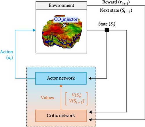
The hyperparameters in the training process of the A2C algorithm include the weights for both the actor and critic network loss functions, the discount rate γ, and the learning rate η.

3. Design of Injection Schedules With A2C

This section outlines the strategies proposed for deriving periodic injection schedules based on operational constraints for safe CO₂ geological storage in saline aquifers considering the geological model and operational conditions, such as fault pressure constraints. Details regarding the settings and criteria for the A2C algorithm components, including the environment, state, action, reward system, and neural networks are provided in this section.

3.1. Geological CO₂ Storage Modeling

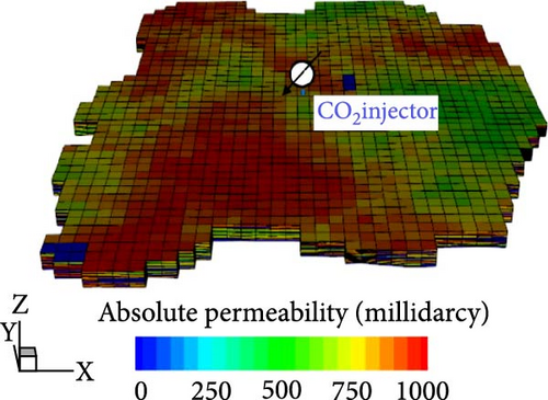
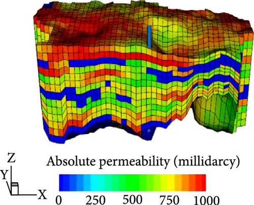
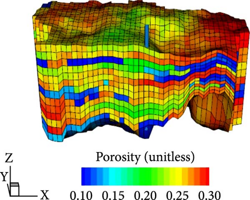
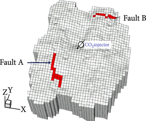
A 3D heterogeneous saline aquifer was generated using geostatistical property modeling (Figure 2); the porosity, absolute permeability, and shale volume of the system are listed in Table 1. The target aquifer for geological CO₂ storage was slightly confined, with a thickness of ~250 m, located between the true vertical depths of 840 and 1090 m. The reference pressure at the top of the aquifer and bottom of the overlying impermeable caprock was 9000 kPa at 840 m. The aquifer, with dimensions (x, y, z) of (6310, 7076, 250 m), consisted of 22,230 unstructured grids (38 × 45 × 13) and showed an average horizontal permeability of 630 millidarcies (md), average porosity of 0.235, and a Dykstra–Parsons coefficient of permeability value of 0.855, indicating high spatial heterogeneity. Moreover, the aquifer contained interbedded shale layers that facilitated trapping at various locations.

Table 1. Reservoir properties and operational conditions for modeling CO₂ geological storage.

Parameter	Value	Unit
Initial pressure (reference pressure)	9000 (at 840 m)	kPa
Average porosity	0.235	—
Average horizontal permeability	630	md
Average vertical permeability	315	md
Shale volume ratio	20	%
Temperature	49.875	°C
Salinity	10,000	ppm
Dykstra–Parsons coefficient	0.855	—
Maximum injection rate	400,000	m³/day
Upper limit for BHP	12,000	kPa
Pressure to activate a fault	11,000	kPa

A single CO₂ injection well was installed at the center of the aquifer with a maximum daily injection rate of 400,000 m³/day under surface conditions and a maximum allowable bottomhole pressure (BHP) of 12,000 kPa. For containment analysis, two faults (A and B) were positioned near the boundaries with an assumed activation pressure of 11,000 kPa (Figure 2d). In the proposed model, CO₂ injection was restricted to facilitate halting when the pressure at either fault attained the activation pressure, while the BHP was maintained below the maximum allowable value of 12,000 kPa. This assumption was designed to support long-term operational strategies by mitigating leakage risks associated with fault activation. With the exception of the fault-activation constraint, the analysis neglected geomechanical features, such as fault deformation, changes in the pore structure, and stress variations.

Designing a periodic CO₂ injection schedule involves formulating a strategy for CO₂ injection at 4-month intervals to maximize the cumulative injection volume over a 16-year period without triggering fault activation. To meet the required criteria, 48 distinct injection rates were assigned over a total period of 16 years.

3.2. Design of A2C

The A2C algorithm uses numerical simulations of a saline aquifer geological model to represent the environmental dynamics of the system. Key observations, such as the BHP and fault pressure, are used to define the state space; the state is represented as a tensor of stacked past observations. Actions are determined within a continuous space guided by the parameters of a normal distribution generated by the actor network. Here, the reward functions were designed to maximize the CO₂ injection amount while controlling the fault pressure. The training process used batch learning with specific configurations to optimize the network performance.

3.2.1. Environment

The dynamics of fluid flow in porous media are typically governed by partial differential equations (PDEs) that indicate the mass and energy balance in each grid block. This study used a model-free reinforcement learning approach, treating PDEs as elements with which the agent interacts at each time step, not as targets for the agent to learn, considering them as a black box. A compositional reservoir simulator solved these PDEs at each time step [30]. Despite the feasibility of training a surrogate model to approximate the state transitions of the environment, enabling relatively rapid predictions and frequent interactions with the agent, this study did not adopt this approach. Owing to training with data derived from PDEs, such surrogate models can introduce prediction errors that tend to accumulate, particularly in high-dimensional and heterogeneous geological models, thereby hindering optimal outcomes in long-term operations involving continuous actions. To ensure accuracy in such complex settings, this study relied on direct interactions with the PDE-based simulator rather than a surrogate model.

3.2.2. States

To record the history of control processes or operations, the state space of the geological model should be able to contain sufficient information or observations, consistent with the assumptions of an MDP. Defining large-scale parameters, such as the distribution of CO₂ pressure or saturation across the entire geological model, as observations for each state would lead to high-dimensional input data (N_obs), increasing the complexity of the neural network required to extract key features; this increases the computational effort required to train the agent significantly. Therefore, this study defined the state using a BHP that is directly affected by the injection activities, and the average fault pressure was monitored to ensure safe injection without fault activation. Including the amount or rate of change of key observations in the state enables the agent to record the momentum and trends in agent/environment interactions [31, 32]. Therefore, the state at a specific time t consists of the following seven elements (N_obs = 7):

(6)

In Equation (6), BHP_t represents the BHP at time step t, while and denote the average pressure at Faults A and B, respectively, at time step t. Each variable was normalized between 0 and 1 based on a BHP upper limit of 12,000 kPa and average fault pressure threshold of 11,000 kPa (Table 1). Elements related to these changes were calculated by subtracting the previous observations from the current observations. and represent changes in the average pressure for Faults A and B, respectively, while Δq_t refers to the change in the normalized daily injection rate. The term t/t_target indicates the temporal position of the current injection point with respect to the target control period (i.e., t_target = 48).

A sequence of past information leading to the current state can enable an agent to understand the dynamic changes in the environment [33]. Here, multiple states from different time steps were treated as history; a total of N_history states were stacked to form the input data for the neural network. The state vector S_t defined in Equation (6) was combined with the three previous state vectors, S_t−1, S_t−2, and S_t−3, to form a matrix of size (7, 4) that was used as input data for the actor and critic neural networks. With time, each new state vector sequentially replaced the oldest state vector in the input data; N_history was set to four.

3.2.3. Actions

This study defined a continuous action space that enabled the agent to select actions freely within the maximum and minimum CO₂ injection ranges by considering the output of the actor network in the A2C algorithm to be the mean (μ) and standard deviation (σ) of a normal distribution, N(μ, σ²); the mean and standard deviation determined the magnitude of the action and exploration range, respectively. Subsequently, the action of the agent in the next state was determined by sampling from this normal distribution.

Directly exploring a wide solution space, such as daily injection rates of up to 400,000 m³/day, is generally unsuitable for the backpropagation process in neural networks. To overcome this limitation and ensure proper learning within the A2C algorithm, the action range sampled from the normal distribution, guided by the actor network, was normalized. The relationship between the range of actions explored by the actor network and actual injection rate can be defined by Equation (7), as follows:

(7)

In Equation (7), a represents the value sampled from the normal distribution generated by the actor network output, q_{real_ max} represents the maximum daily injection rate (400,000 m³/day), q_{real_ min} is the minimum daily injection rate (10 m³/day), and q_real refers to the actual injection rate applied to the environment, which ranges within 10–400,000 m³/day.

3.2.4. Reward Functions

Three distinct reward systems were examined in this study: Reward A (R(A)), a system based on the amount of CO₂ injected until the activation of one fault; Reward B (R(B)), a system which extends R(A) by adding a scalar value as the control or injection period extends; and Reward C (R(C)), a system that builds on R(B), with an additional reward granted if the injection duration reaches the targeted injection period of 16 years. The total rewards accumulated over an episode until the stopping criterion (t_max) was attained, representing the “score,” which indicates the effectiveness of the A2C algorithm. The score for each reward system can be defined by the following equations:

(8)

(9)

(10)

In the above equations, C_t represents the volume of CO₂ injected during an individual time step, i.e., within 4 months, and the constants α, τ, and β scale the rewards to ensure the reliability of the training process. Based on the mean daily injection rate (200,000 m³/day; Table 1), ~2.43 × 10⁷ m³ of CO₂ was injected over a 4-month period. Therefore, α was set to 2.00 × 10⁻⁹ to adjust the reward value for C_t to ~0.05. τ was set to 0.05, aligning its scale with α × C_t, and β was set to 1.25 to ensure that the additional reward—proportional to the total injected amount after the targeted injection period—was comparable in magnitude to R(B)_score. For R(C), if any fault was activated before the 16-year mark, a negative reward of −1 was applied.

3.2.5. Training Process

The A2C architecture with tensor-stacking state vectors (N_obs = 7 and N_history = 4) is shown in Figure 3. At each time step, new observations replace the oldest column of data in the existing tensor. The He-normal initializer [34] implements neural networks for both the actor and critic. Here, each network underwent two convolutional operations with 32 kernels (kernel size: 2 × 2; stride: 2 × 2; and activation function: LeakyReLU [35]). Subsequently, the output was processed through a fully connected layer with 24 nodes using a sigmoid activation function for the actor and a linear function for the critic.

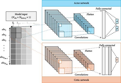
Value function estimation is more complex than action selection and requires precise feedback for policy updates; therefore, an additional fully connected layer with 24 nodes was used in the critic network to improve its value estimation accuracy. A total of 15,443 parameters was used in the two neural networks, rendering the structure relatively simple and computationally efficient.

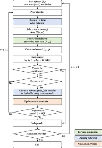
The training workflow of the A2C-based injection scheduling is shown in Figure 4. In this study, a set of states S_t, action q_t, reward r_t+1, and the next state S_t+1 at a specific time step t within a given episode E_i is considered to be a single sample. Samples from the same episode were stored in a buffer, and the collection of a predetermined number of samples was followed by batch training. The networks were updated after the accumulation of 12 samples. This approach considers the long-term behavior of the environment, particularly delayed rewards, and addresses the limitations of the baseline A2C, which updates the actor and critic networks at each time step, relying only on the most recent information.

Among the hyperparameters of the training procedure, the weight of the actor network loss function (Equation (4)) was set to 0.1 and added to the loss function of the critic network (Equation (5)). The A2C algorithm was trained by minimizing the combined loss function using the Adam optimizer [36] with a η (Equation (3)) of 0.0005. The value of γ in Equation (2) was considered to be 0.985.

4. Results and Discussion

The performance and reliability of the proposed framework for developing a secure CO₂ injection schedule under operational constraints were validated through designing a suitable reward system and conducting a thorough analysis of the selected injection schedule. Additionally, the applicability of the framework to environments with uncertainty was assessed, and potential directions for future research were explored.

4.1. Validation of the Proposed Framework Under Different Reward Systems

Three distinct cases based on the components of the Reward A system, as outlined in Section 3.2.4, were considered: Reward A, which is based on the amount of CO₂ injected (Equation (8)), Reward B, which includes a scalar reward on increasing the control or injection period (Equation (9)), and Reward C, which incorporates an additional reward based on the attainment of the targeted injection period (Equation (10)). This section discusses the training trends and selected injection schedules to identify the optimal reward system.

4.1.1. Evaluation of the Training Trend of the A2C Algorithm

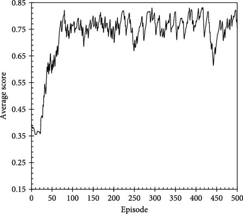
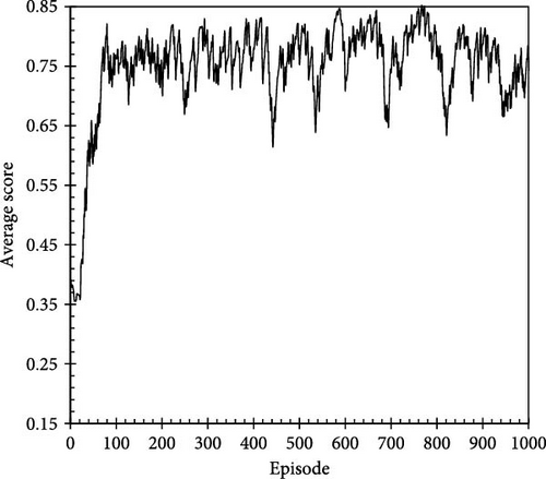
The average score was calculated using an exponentially weighted moving average (EWMA), which assigns a weight of 0.9 to the previous score and 0.1 to the new score. This method gradually reduces the influence of older scores, expediting the reflection of current trends. Figure 5a shows the results of training the A2C algorithm with Reward C over 500 episodes, with each average score normalized by the maximum score. With training, the average score steadily increases, stabilizing within the range of 0.75–0.8 after ~100 episodes, indicating that the agent effectively learns to generate preferred action trajectories within a large continuous action space. Reinforcement learning focuses on training the agent to explore various actions and progressively favors the actions that yield higher scores. The shape of the average score profile in Figure 5 indicates that the agent learned from repeated interactions with the environment to select higher-reward actions, resulting in a stable training performance [20, 28, 33]. This trend continued even when the training was extended to 1,000 episodes (Figure 5b). The slight oscillation in the average score can be attributed to the stochastic nature of sampling actions from a continuous action space and the variability in delayed rewards specific to each episode under Reward C.

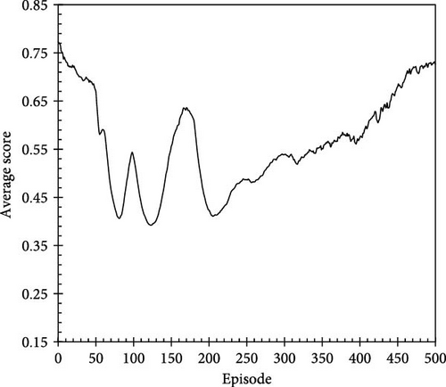
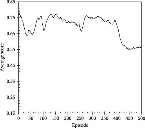
The trends of the average score over 500 training episodes for the other reward systems, i.e., Reward A (Figure 6a) and Reward B (Figure 6b), are shown in Figure 6. To compare the scores across the different reward systems quantitatively, Equations (8) and (9) were used to scale the results for Rewards A and B based on using the maximum score attained in Reward C as a reference. Figure 6 indicates that the performance of the agent under Rewards A and B did not show a stabilizing trend in the average score; moreover, the performance did not significantly improve compared with the initial episodes. These results highlight the importance of incorporating elements that reflect delayed responses toward the environment into the reward system; reward systems lacking appropriate feedback for action trajectories make it challenging for an agent to explore a globally optimal solution that adheres to operational constraints. Furthermore, after ~100 episodes of training, the average scores for Reward C (Figure 5a) were generally higher than those observed for Rewards A and B, confirming the higher efficacy of the action trajectories or injection scenarios under Reward C in terms of both the injected volume and duration.

4.1.2. Comparative Analysis of Injection Schedules

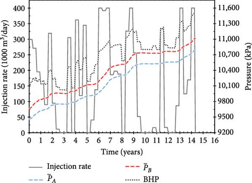
This section compares the results of each reward system by examining the action trajectories and several injection schedules, highlighting the excellent performance of Reward C. Figure 7 shows the CO₂ injection rate (black solid lines) and monitoring parameters over time, specifically BHP (black dotted lines) and the average pressure of Faults A (blue dashed lines) and B (red dashed lines), for episodes with the maximum score during training under Rewards A and B. The injection schedules under these two reward systems were assessed for injecting 854 million cubic meters (MM m³) (Reward A) and 887 MM m³ (Reward B) of CO₂. However, in both cases, the pressure in Fault B exceeded the critical value of 11,000 kPa after 14 years and 4 months for Reward A and 14 years and 5 months for Reward B (Figure 7a,b). These results indicate that Rewards A and B are inadequate for deriving a safe injection schedule over the targeted injection period, consistent with the analysis described in the previous section.

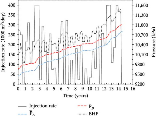
Figures 8 and 9 show the CO₂ injection rates, BHPs, and average fault pressures over time for several injection scenarios developed during the training process based on Reward C (as shown in Figure 5a). The injection scenarios from the early stages of training failed to achieve the target injection period, resulting in penalties as delayed rewards. Specifically, in the 2^nd episode, 742 MM m³ of CO₂ was injected over 29 control periods (Figure 8a); in the 8^th episode, 696 MM m³ was injected over 29 control periods (Figure 8b); and in the 49^th episode, 788 MM m³ was injected over 34 control periods (Figure 8c). Because the pressure at Fault B exceeded the critical value during these control periods, the scores for these three scenarios were 1.84, 1.79, and 2.16, respectively.

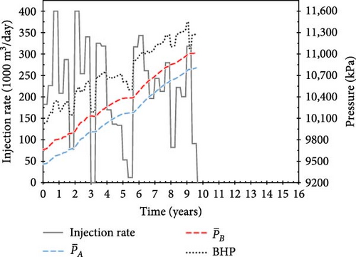
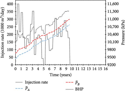
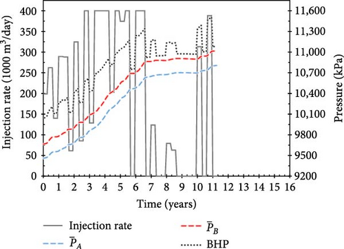
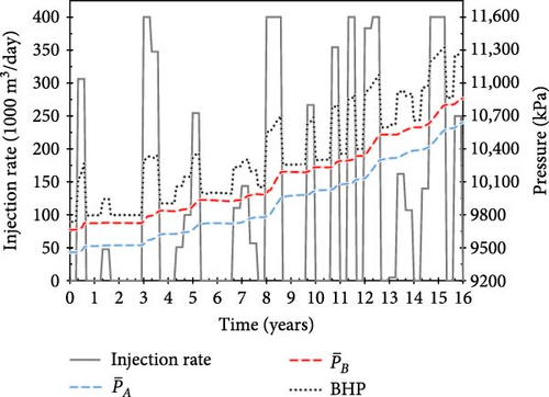
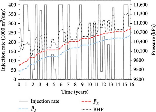
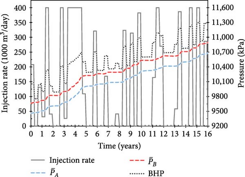
With training, the agent develops injection scenarios that maintain the average fault pressure below the critical value, thereby earning additional positive rewards proportional to the total amount of CO₂ injected (Equation (10)). Figure 9a–c shows examples of operational scenarios that achieved the target injection period; the scenarios, with scores of 5.46, 6.41, and 5.95, respectively, injected 717, 959, and 830 MM m³ of CO₂, respectively, over 16 years.

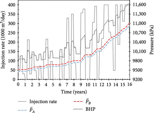
Notably, the injection schedule gradually evolved from a strategy with a tendency to continuously inject large amounts of CO₂ (Figure 8) to one with minimal injection rate (10 m³/day) periods (Figure 9). Although the amount of CO₂ injected during “buffer periods” (with minimal injection rates) is minimal, their strategic placement between injection schedules helps mitigate increasing pore-pressure trends and pressure propagation in the saline aquifer caused by previous actions. Therefore, the proposed approach enables the fault pressure to be maintained below the critical value. Figure 9b shows the scenario with the highest score across all reward systems, which injects the largest amount of CO₂ (959 MM m³) over a 16-year injection period.

Table 2 shows that Reward C leads to the most reliable and meaningful results among all the tested reward systems. When a reward system includes both the reward associated with each control period and feedback on the trajectory of actions, the A2C algorithm shows stable learning trends and effectively derives an injection scenario that maximizes CO₂ injection within operational constraints. The baseline A2C algorithm, which updates the neural network at each time step using only the BHP and average fault pressure as the state of the environment under Reward C, is detailed in the Appendix.

Table 2. Summary of the selected scenarios under different reward systems.

Reward system	Injectable period	Cumulative injected volume (MM m³)	Fault B pressure at the last monitoring time (kPa)
Reward A	14 years and 4 months	854	11,014
Reward B	14 years and 5 months	887	11,002
Reward C	16 years	959	10,837

4.2. Effectiveness of the CO₂ Injection Schedule Proposed by the A2C Algorithm

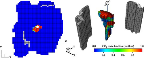
The optimal periodic CO₂ injection strategy proposed by A2C (Figure 9b) maximizes the cumulative CO₂ amount over 16 years without activating any fault. If the CO₂ plume—movable CO₂ migrating through pores—reaches a fault after activation, the risk of leakage may increase. Figure 10 shows the gas mole fraction of the injected CO₂, showing the CO₂ plume after 8, 16, and 50 years of injection. Upon reaching the impermeable caprock, the injected CO₂ spreads extensively beneath it, migrating from the injection well to Fault A with relatively high permeability. Figure 10b,c indicates that the injected CO₂ does not reach Fault A by the end of the injection schedule (16 years); however, the mobile plume may reach Fault A at around the 50^th year. As Fault A remains inactive, CO₂ storage is maintained without leakage through the fault aperture. Despite uncertainties regarding fault sealing, the simulation results confirm geological containment under these conditions for a minimum period of 50 years.

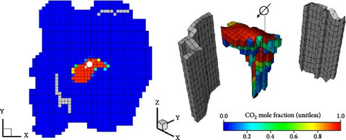
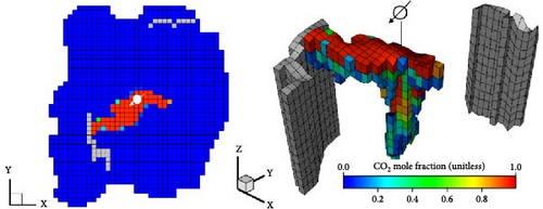
To assess the effectiveness of the proposed periodic schedule, this study compared the cumulative CO₂ injection volume and operational period of the proposed schedule with those of a constant-injection-rate scenario. The constant injection rate was estimated to be 164,174 m³/day by dividing the total amount of CO₂ injected by the duration of the injection period (16 years), i.e., the calculated value is the average daily rate for the optimal periodic strategy (Figure 9b).

The pressure increase in the optimal periodic strategy and the constant-injection-rate scenario are compared in Figure 11. The pressure increases relatively rapidly in the constant-injection-rate scenario, causing the activation of Fault A within 13.3 years (13 years and 4 months from the start of injection) and Fault B within 11.3 years. Owing to the operational constraint of halting injection when the activation pressure is measured at either fault, the constant-injection case is expected to end at 11.3 years. Within this period, the cumulative injected volume (674 MM m³) is 70.3% of the optimal volume (959 MM m³) (Figure 12). This result confirms the high efficacy of the proposed optimal schedule, which extends the injection period by 4.7 years, thereby increasing the cumulative injected volume by ~ 30%.

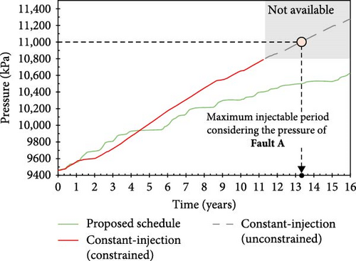
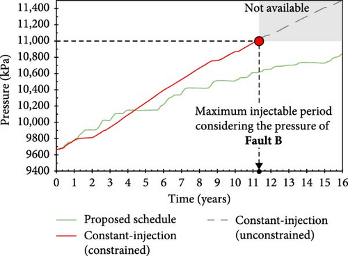
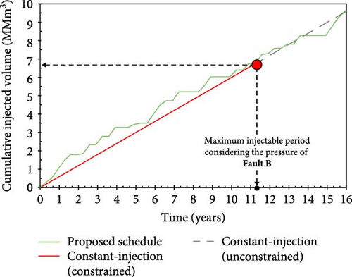
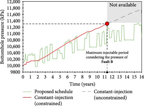
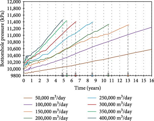
Figure 13 and Table 3 show the injection termination times and cumulative injection volumes of various constant-injection-rate schedules. As the daily injection rate increases, the pressure in the aquifer increases more rapidly. Consequently, the time required to reach the fault activation pressure is reduced, which in turn lowers the cumulative injection volume. For instance, at an injection rate of 400,000 m³/day, the cumulative volume over 4 years and 11 months is ~706 MM m³. In comparison, the largest cumulative injection volume achieved with a constant rate is 784 MM m³—77.7% of the optimal injectable volume—over 8.7 years at a rate of 250,000 m³/day. Therefore, the A2C-based optimal periodic schedule proposed in this study outperforms the constant-rate strategy, showing 22.3% greater CO₂ injectable volumes while maintaining fault stability. Compared with scenarios with constant CO₂ injection rates, the A2C-based periodic CO₂ injection design provides advantages in terms of both cumulative injection volume and duration, while ensuring containment.

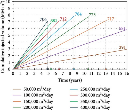
Table 3. Comparison of the injection period and cumulative volume for various constant-injection-rate cases.

Constant injection rate (m³/day)	Injectable period	Cumulative injectable volume until activating any fault (MM m³)
50,000	16 years	291
100,000	16 years	581
150,000	13 years and 2 months	717
200,000	10 years and 8 months	773
250,000	8 years and 8 months	784
300,000	6 years and 7 months	712
350,000	5 years and 5 months	681
400,000	4 years and 11 months	706

4.3. Applicability Under Geological Uncertainty

Despite the precise modeling of the environmental dynamics in CO₂ injection projects through computational simulations, accounting for all uncertainties that arise in on-site field operations remains challenging. For maximum safety, incorporating uncertainties due to additional weak zones or faults that might be activated by injection activities into injection scheduling is critical. This section evaluates the practicability of the reinforcement learning-based framework developed in this study. Training the A2C algorithm under various environments enables the proposed framework to function accurately in uncertain cases that differ from those encountered in the training process.

This framework enables the probabilistic determination of the injection rate at each time step within a continuous action space, permitting the generation of additional operational scenarios using the trained algorithm. Figure 14 shows the average score trends for 100 testing episodes, which are additional scenarios derived from the A2C algorithm trained in Section 4.1. The scaled average score ranges within 0.75–0.80, consistent with the results shown in Figure 5. The operational scenarios during the testing episodes show an average injection period of 15 years and 3 months, with an average injected CO₂ volume of 724 MM m³ and standard deviation of 109 MM m³. The P10, P50, and P90 scenarios—based on total injection volumes—attain the targeted injection period, allowing for the injection of 843, 733, and 583 MM m³ of CO₂, respectively. These results demonstrate that the developed framework can reliably suggest additional candidate scenarios and exhibits high potential to facilitate the selection of an appropriate injection schedule based on the total amount of CO₂ to be injected.

Although the stochastic nature of sampling actions from a continuous space enables the generation of diverse operational scenarios, designing a system for monitoring optimization while considering environmental uncertainty remains a significant challenge. This study examined the robustness of the proposed A2C-based method by testing the training processes for different fault locations (i.e., under environmental uncertainty).

Figure 15 shows the fault locations in the environments used in this study. The geological model described in Section 4.1(Figure 2d) was used as the Base Case; the new geological models incorporated additional fault grids into the Base Case (Figure 15a–c). Figure 15c shows the geological model used to test the trained agent; compared with the other geological models, this model contains additional fault grids on the opposite side. Owing to high variability in flow-related parameters, such as permeability and porosity, pressure changes in the aquifer are not simply proportional to the distance between the injection well and the fault. Therefore, the additional grids were considered as extensions of existing faults (rather than separate faults). Specifically, the fault grids south of the injection well were labeled as Fault A, whereas those to the north were labeled as Fault B.

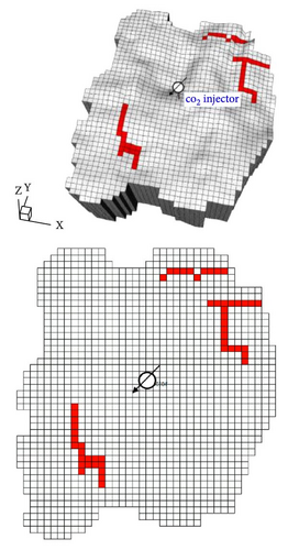
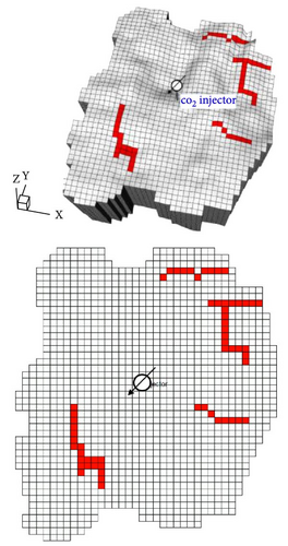
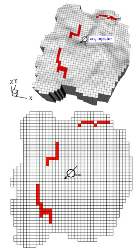
In this case study, the agent was trained by interactions with a different geological model in each episode. The settings for the state, reward system, and neural network architecture are consistent with the settings described in Section 4.1. Figure 16a shows the scaled trend of the average score over 1500 episodes, and Figure 16b shows the trends for each geological model during the training process. All the geological models show similar average score trends because the monitoring locations in Cases A and B are based on the positions of existing faults in the Base Case.

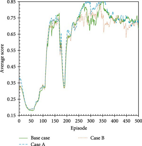
The average score of the A2C algorithm stabilizes at ~0.75 after ~750 training episodes across different geological models (~250 episodes per geological model). Although the number of episodes required for stable learning is slightly higher than that indicated by the results described in Section 4.1, the algorithm is trained to establish schedules that enable adequate CO₂ injection within the targeted injection period across various environments.

Figure 17 shows the injection scenarios with the highest scores for each geological model during the training process. The training process, which accounts for uncertainty, effectively derives cyclic injection schedules tailored for each geological model. The estimated cumulative CO₂ injection volumes for the Base Case, Case A, and Case B are 841, 874, and 841 MM m³, respectively. Notably, in this case study, the injection volume for the Base Case is ~87.7% of the volume evaluated in Section 4.1; this reduction possibly occurs because the algorithm used in this case study is trained across geological models that include areas closer to the injection well, leading to a more conservative policy than that specific to a single geological model.

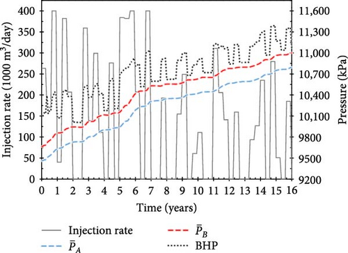
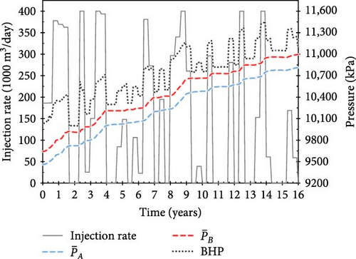
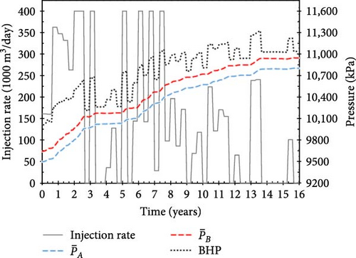
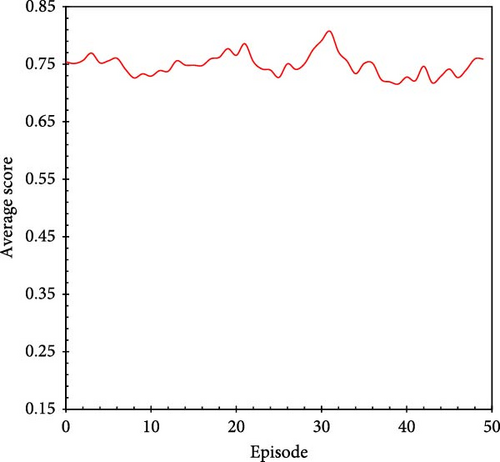
Figure 18 shows the trend of the scaled average score over 50 episodes while evaluating the trained algorithm in the test environment (Figure 15c). The average score stabilizes at ~0.75, consistent with the results shown in Figure 14, indicating that the developed framework can be effectively applied to geological models that are not used during training. In these test episodes, the average injection period, average injection volume, and standard deviation are ~15 years and 11 months, 638, and 194 MM m³, respectively. According to total injection volume calculations, the P10, P50, and P90 scenarios enable the injection of 882, 648, and 363 MM m³ of CO₂, respectively, within a 16-year injection period. Figure 19 shows the scenario with the highest score among the test episodes, confirming the maximum safe CO₂ injection volume for the Case C geological model to be 914 MM m³.

4.4. Challenges for Future Research

This study developed a framework to explore optimal operating scenarios for a single CO₂ injection well under geological uncertainty. In addition to the work described in Section 4.1 and the Appendix, the main challenge was to define an appropriate criterion for the A2C model, including the selection of suitable hyperparameters. Specifically, it may be possible to enhance the analyses related to the definitions of the state (or observation), reward system, scale factor, and weight distribution of the neural networks. These challenges are inherent to reinforcement learning and are further amplified in complex geosystems, where evaluating agent interactions requires significant computational resources.

Future research should focus on extending this study to larger-scale problems, such as multi-well operations and other geosystems such as depleted gas reservoirs. It should also aim to integrate transport, injection, and storage facilities within a comprehensive system. This would require detailed investigations of various operational constraints and monitoring parameters, including geomechanics, thermal parameters, caprock integrity, reservoir fracture pressure, well stability, and flow assurance. By leveraging the model-free nature of the A2C algorithm, incorporating real-time sensor data from distributed temperature sensing, permanent drilling pressure and temperature gauges, and other sensors into the reinforcement learning framework could improve its effectiveness. Integrating extensive raw sensor signals using supervised learning (to convert raw data into processed forms) or unsupervised learning (to extract low-dimensional latent features) may provide valuable insights.

To facilitate rapid environmental response predictions, future studies should implement advanced surrogate models. Recurrent neural networks or convolutional long short-term memory networks can estimate sequential transitions in the environment [27], although their reliability depends on the size of the available dataset. Alternatively, physics-informed neural networks or deep operator networks, which are mesh-free and rely on physics-based data to solve PDEs of the environment, could be viable options [37–39].

Exploring alternative reinforcement learning algorithms could address challenges related to sample efficiency and dependency. For example, the soft actor-critic algorithm, i.e., an off-policy approach, could improve sample efficiency by reusing past experiences [40]. The asynchronous advantage actor–critic algorithm, which employs multiple agents simultaneously, can reduce dependency among training samples and help mitigate optimization challenges in high-dimensional geosystems [41].

In summary, a comprehensive analysis of geological settings tailored to target storage sites, along with a thorough consideration of monitoring and uncertainty parameters, is crucial. Developing solutions to improve the scalability and efficiency of reinforcement learning algorithms remains a priority. Advanced methodologies, such as integrating large language models (LLMs) [42] without human supervision—particularly for designing reward systems—could offer significant advancements.

5. Conclusions

This study developed a deep reinforcement learning-based framework utilizing the A2C algorithm to address the challenges of CO₂ geological storage under operational constraints, such as fault activation. By appropriately configuring the reward system, state vector, and training process, the framework can effectively derive injection scenarios consisting of injection rates sampled from a continuous action space. The proposed framework shows stable learning trends with a reward system that considers the cumulative injectable CO₂ amount, injection duration, and feedback from the trajectory of actions.

The injection scenario proposed in this study involves significant improvements in the cumulative injectable amount of CO₂ over a 16-year period, injecting up to 959 MM m³ of CO₂, which is 22.3% higher than the maximum CO₂ volume injected in constant-injection scenarios. The applicability of the proposed framework under geological uncertainties was confirmed through reliable periodic injection scenarios tailored to different fault locations. The framework effectively adapted and maintained stable performance, even under unique environments not encountered during training. Therefore, the proposed framework for optimizing CO₂ injection strategies shows robustness, balancing the CO₂ storage efficiency with operational constraints and environmental uncertainties.

The proposed method is expected to expedite the development of efficient operational strategies for CO₂ geological storage projects. Moreover, the method exhibits high potential to address additional monitoring parameters, such as caprock integrity, and optimize complex scenarios involving surface facilities, or multiwell operations.

Nomenclature

A2C:: Advantage actor–critic
BHP:: Bottomhole pressure
CO₂:: Carbon dioxide
DQN:: Deep Q-network
EWMA:: Exponentially weighted moving average
kPa:: Kilopascal
LLMs:: Large language models
md:: Millidarcy
MDP:: Markov decision process
MM:: Million
PDEs:: Partial differential equations
TD:: Temporal-difference
a:: Action
C_t:: Volume of CO₂ injected during a time step
E:: Episode
N_obs:: Number of observations
N_history:: Number of historical state data
:: Average pressure at Fault A
:: Average pressure at Fault B
q:: Normalized injection rate of CO₂
Q:: Action-value function
q_real:: Actual injection rate of CO₂
q_{real_ max}, q_{real_ min}:: Maximum and minimum injection rates of CO₂
r:: Reward
R:: Reward system
R_score:: Total rewards accumulated over an episode
S:: State
t:: Time step
t_max:: Time at the stopping criterion in an episode
t_target:: Target control period
V:: Value function
α, β:: Scale factor
γ:: Discount rate
δ_ω:: Advantage function in terms of temporal-difference error
η:: Learning rate
θ:: Weight parameter of actor network
μ:: Mean of normal distribution
π:: Policy
σ:: Standard deviation of normal distribution
τ:: Scalar reward for duration of injection
ω:: Weight parameter of critic network

Abbreviations

A2C:: Advantage actor–critic
MDP:: Markov decision process
DQN:: Deep Q-network
TD:: Temporal-difference
BHP:: Bottomhole pressure
PDEs:: Partial differential equations
EWMA:: Exponentially weighted moving average.

Conflicts of Interest

The authors declare that this study was conducted in the absence of any commercial or financial relationships that could be construed as potential conflicts of interest.

Author Contributions

Suryeom Jo: Conceptualization, methodology, software, validation, investigation, formal analysis, visualization, writing – original draft preparation, writing – review, and editing. Tea-Woo Kim: Validation, investigation, visualization, writing – original draft preparation, and writing – review, and editing. Changhyup Park: Conceptualization, validation, investigation, formal analysis, visualization, writing – original draft preparation, writing – review, and editing. Byungin Choi: Methodology and software.

Funding

This research was supported by the Ministry of Trade, Industry, and Energy (MOTIE) (No. 20212010200020) and Korea Institute of Geoscience and Mineral Resources (KIGAM) (GP2025-017; GP2025-021), Korea.

Appendix A: Training Results for the Baseline A2C Algorithm

This appendix includes the results of training a baseline or “vanilla” A2C algorithm, which updates the neural network at each time step using only basic observational data. The environmental settings and reward system are consistent with those described in Section 4.1.

The state consists solely of the BHP and the pressures of the two faults (A and B); it does not incorporate historical data (which accumulate multiple states) or batch training (which uses samples within the same episode). Specifically, the input data for the two neural networks in the A2C algorithm comprises three dimensions. Each network processes the data through two fully connected layers, each with 24 nodes. The actor network outputs the mean (μ) and standard deviation (σ) of the normal distribution for action sampling, while the critic network outputs the state-value estimate. The real action value input to the environment, denoted as q′_real, is determined using the following equation:

(A.1)

where a′ represents the action value derived from the output of the actor network and is set to allow values up to four times larger than in previous cases. The maximum and minimum values for q′_real are set to 100,000 and 10 m³/day, respectively, ensuring that the real action values input to the environment range from 10 to 400,000 m³/day, as specified in Equation (7). This configuration aims to assess the results when the actor network explores a relatively wide range of CO₂ injection rates compared with previous scenarios.

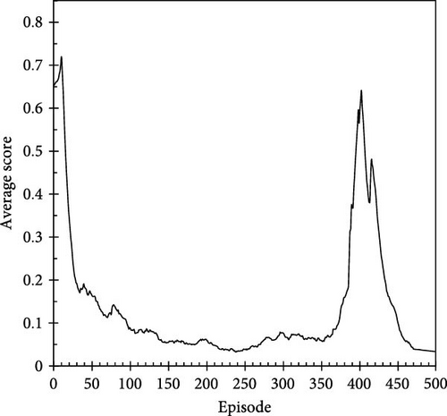
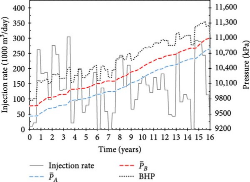
Figure A1 shows the trend of scores during the training process over 500 episodes under the conditions described above. Unlike previous cases, in which interactions with the environment gradually led to stable rewards (Figures 5 and 16), the baseline model did not maintain high scores. This indicates that the baseline model struggled to discover an optimal policy and adapt to the environment. Figure A2 shows the injection scenario that showed the highest score during the training of the baseline model. Notably, the maximum daily injection rate of 400,000 m³/day was not used in any period, and the cumulative CO₂ volume was calculated to be 810 MM m³, which is ~84.5% of the maximum injection volume evaluated in Section 4.1.

Open Research

Data Availability Statement

Data supporting the findings of this study are available upon reasonable request.

References

1 Ajayi T., Gomes J. S., and Bera A., A Review of CO₂ Storage in Geological Formations Emphasizing Modeling, Monitoring and Capacity Estimation Approaches, Petroleum Science. (2019) 16, no. 5, 1028–1063, https://doi.org/10.1007/s12182-019-0340-8, 2-s2.0-85068843144.
10.1007/s12182-019-0340-8
CAS Web of Science® Google Scholar
2 Ringrose P., How to Store CO2 Underground: Insights From Early-Mover CCS Projects, 2020, Springer International Publishing, Cham, https://doi.org/10.1007/978-3-030-33113-9.
10.1007/978-3-030-33113-9
Google Scholar
3 Miri R. and Hellevang H., Salt Precipitation During CO₂ Storage—A Review, International Journal of Greenhouse Gas Control. (2016) 51, 136–147, https://doi.org/10.1016/j.ijggc.2016.05.015, 2-s2.0-84971623044.
10.1016/j.ijggc.2016.05.015
CAS Web of Science® Google Scholar
4 Ahmad S., Li Y., Li X., Xia W., Chen Z., and Ullah N., Numerical Analysis of CO₂ Hydrate Growth in a Depleted Natural Gas Hydrate Formation With Free Water, Greenhouse Gases: Science and Technology. (2019) 9, no. 6, 1181–1201, https://doi.org/10.1002/ghg.1924, 2-s2.0-85073773815.
10.1002/ghg.1924
CAS Web of Science® Google Scholar
5 Cui G., Hu Z., Ning F., Jiang S., and Wang R., A Review of Salt Precipitation During CO₂ Injection Into Saline Aquifers and Its Potential Impact on Carbon Sequestration Projects in China, Fuel. (2023) 334, https://doi.org/10.1016/j.fuel.2022.126615, 126615.
10.1016/j.fuel.2022.126615
CAS Google Scholar
6 Aghajanloo M., Yan L., Berg S., Voskov D., and Farajzadeh R., Impact of CO₂ Hydrates on Injectivity During CO₂ Storage in Depleted Gas Fields: A Literature Review, Gas Science and Engineering. (2024) 123, https://doi.org/10.1016/j.jgsce.2024.205250, 205250.
10.1016/j.jgsce.2024.205250
CAS Web of Science® Google Scholar
7 Jung H., Singh G., Espinoza D. N., and Wheeler M. F., Quantification of a Maximum Injection Volume of CO₂ to Avert Geomechanical Perturbations Using a Compositional Fluid Flow Reservoir Simulator, Advances in Water Resources. (2018) 112, 160–169, https://doi.org/10.1016/j.advwatres.2017.12.003, 2-s2.0-85039162747.
10.1016/j.advwatres.2017.12.003
CAS Web of Science® Google Scholar
8 Newell P. and Martinez M. J., Numerical Assessment of Fault Impact on Caprock Seals During CO₂ Sequestration, International Journal of Greenhouse Gas Control. (2020) 94, https://doi.org/10.1016/j.ijggc.2019.102890, 102890.
10.1016/j.ijggc.2019.102890
CAS Web of Science® Google Scholar
9 Edlmann K., Hinchliffe S., Heinemann N., Johnson G., Ennis-King J., and McDermott C. I., Cyclic CO₂ – H₂O Injection and Residual Trapping: Implications for CO₂ Injection Efficiency and Storage Security, International Journal of Greenhouse Gas Control. (2019) 80, 1–9, https://doi.org/10.1016/j.ijggc.2018.11.009, 2-s2.0-85057103134.
10.1016/j.ijggc.2018.11.009
CAS Web of Science® Google Scholar
10 Shchipanov A., Kollbotn L., Encinas M., Fjelde I., and Berenblyum R., Periodic CO₂ Injection for Improved Storage Capacity and Pressure Management Under Intermittent CO₂ Supply, Energies. (2022) 15, no. 2, https://doi.org/10.3390/en15020566, 566.
10.3390/en15020566
CAS Google Scholar
11 Li S., Wang P., Wang Z., Cheng H., and Zhang K., Strategy to Enhance Geological CO₂ Storage Capacity in Saline Aquifer, Geophysical Research Letters. (2023) 50, no. 3, https://doi.org/10.1029/2022GL101431, e2022GL101431.
10.1029/2022GL101431
CAS Web of Science® Google Scholar
12 Sawada Y., Tanaka J., Suzuki C., Tanase D., and Tanaka Y., Tomakomai CCS Demonstration Project of Japan, CO₂ Injection in Progress, Energy Procedia. (2018) 154, 3–8, https://doi.org/10.1016/j.egypro.2018.11.002, 2-s2.0-85065961587.
10.1016/j.egypro.2018.11.002
CAS Google Scholar
13 Cappa F. and Rutqvist J., Modeling of Coupled Deformation and Permeability Evolution During Fault Reactivation Induced by Deep Underground Injection of CO₂, International Journal of Greenhouse Gas Control. (2011) 5, no. 2, 336–346, https://doi.org/10.1016/j.ijggc.2010.08.005, 2-s2.0-79951947371.
10.1016/j.ijggc.2010.08.005
Web of Science® Google Scholar
14 Alexander D. and Boodlal D., Evaluating the Effects of CO₂ Injection in Faulted Saline Aquifers, Energy Procedia. (2014) 63, 3012–3021, https://doi.org/10.1016/j.egypro.2014.11.324, 2-s2.0-84922936190.
10.1016/j.egypro.2014.11.324
CAS Google Scholar
15 Vilarrasa V., Makhnenko R. Y., and Laloui L., Potential for Fault Reactivation due to CO₂ Injection in a Semi-Closed Saline Aquifer, Energy Procedia. (2017) 114, 3282–3290, https://doi.org/10.1016/j.egypro.2017.03.1460, 2-s2.0-85029655282.
10.1016/j.egypro.2017.03.1460
CAS Google Scholar
16 Zheng F., Jha B., and Jafarpour B., Controlled CO₂ Injection Into Storage Reservoirs to Minimize Geomechanical Risks under Geologic Uncertainty, Proceedings—SPE Annual Technical Conference and Exhibition. (2023) https://doi.org/10.2118/215155-MS.
10.2118/215155-MS
Google Scholar
17 Mortazavi A. and Maratov T., Investigation of Fault Activation Mechanisms in Carbon (CO2) Storage, 2023, Al Khobar, Saudi Arabia, International Geomechanics Symposiumhttps://doi.org/10.56952/IGS-2023-0009.
10.56952/IGS-2023-0009
Google Scholar
18 Yoon S., Lee H., and Kim J., The Modeling of Fault Activation, Slip, and Induced Seismicity for Geological CO₂ Storage at a Pilot-Scale Site in the Janggi Basin, South Korea, International Journal of Rock Mechanics and Mining Sciences. (2023) 170, https://doi.org/10.1016/j.ijrmms.2023.105441, 105441.
10.1016/j.ijrmms.2023.105441
Google Scholar
19 Hourfar F., Bidgoly H. J., Moshiri B., Salahshoor K., and Elkamel A., A Reinforcement Learning Approach for Waterflooding Optimization in Petroleum Reservoirs, Engineering Applications of Artificial Intelligence. (2019) 77, 98–116, https://doi.org/10.1016/j.engappai.2018.09.019, 2-s2.0-85055109271.
10.1016/j.engappai.2018.09.019
Web of Science® Google Scholar
20 Sun A. Y., Optimal Carbon Storage Reservoir Management Through Deep Reinforcement Learning, Applied Energy. (2020) 278, https://doi.org/10.1016/j.apenergy.2020.115660, 115660.
10.1016/j.apenergy.2020.115660
Google Scholar
21 Li H. and Misra S., Reinforcement Learning Based Automated History Matching for Improved Hydrocarbon Production Forecast, Applied Energy. (2021) 284, https://doi.org/10.1016/j.apenergy.2020.116311, 116311.
10.1016/j.apenergy.2020.116311
Google Scholar
22 Guevara J. L., Patel R., and Trivedi J., Optimization of Steam Injection in SAGD Using Reinforcement Learning, Journal of Petroleum Science and Engineering. (2021) 206, https://doi.org/10.1016/j.petrol.2021.108735, 108735.
10.1016/j.petrol.2021.108735
CAS Web of Science® Google Scholar
23 Alolayan O. S., Alomar A. O., and Williams J. R., Parallel Automatic History Matching Algorithm Using Reinforcement Learning, Energies. (2023) 16, no. 2, https://doi.org/10.3390/en16020860, 860.
10.3390/en16020860
Google Scholar
24 Abdalla R., Hollstein W., Carvajal C. P., and Jaeger P., Actor-Critic Reinforcement Learning Leads Decision-Making in Energy Systems Optimization—Steam Injection Optimization, Neural Computing and Applications. (2023) 35, no. 22, 16633–16647, https://doi.org/10.1007/s00521-023-08537-6.
10.1007/s00521-023-08537-6
Web of Science® Google Scholar
25 Ma H., Yu G., She Y., and Gu Y., Waterflooding Optimization Under Geological Uncertainties by Using Deep Reinforcement Learning Algorithms, SPE Annual Technical Conference and Exhibition, Society of Petroleum Engineers (SPE), 2019, One Petro, https://doi.org/10.2118/196190-MS.
10.2118/196190-MS
Google Scholar
26 De Paola G., Ibanez-Llano C., Rios J., and Kollias G., Reinforcement Learning For Field Development Policy Optimization, SPE Annual Technical Conference and Exhibition. (2020) https://doi.org/10.2118/201254-MS.
10.2118/201254-MS
Google Scholar
27 Aranguren C. and Aguilera R., Application of Self-Learning Enhancing Huff and Puff Gas Injection Optimization in Shale Reservoirs Through Sequence-Based Proxy Reservoir Simulation and Reinforcement Learning, Geoenergy Science and Engineering. (2024) 234, https://doi.org/10.1016/j.geoen.2024.212676, 212676.
10.1016/j.geoen.2024.212676
CAS Google Scholar
28 Mnih V., Kavukcuoglu K., Silver D., Graves A., Antonoglou I., and Wierstra D., Playing Atari With Deep Reinforcement Learning, 2013, https://doi.org/10.48550/arXiv.1312.5602.
10.48550/arXiv.1312.5602
Google Scholar
29 Sutton R. S., McAllester D., Singh S., and Mansour Y., S. Solla, T. Leen, and K. Müller, Policy Gradient Methods for Reinforcement Learning with Function Approximation, Advances in Neural Information Processing Systems, 1999, 12, MIT Press.
Google Scholar
30 Computer Modelling Group Ltd. CMG-GEM, 2023, Calgary, Alberta, Canada.
Google Scholar
31 Heess N., Wayne G., Silver D., Lillicrap T., Tassa Y., and Erez T., Learning Continuous Control Policies by Stochastic Value Gradients, 2015, https://doi.org/10.48550/arXiv.1510.09142.
10.48550/arXiv.1510.09142
Google Scholar
32 Kiran B. R., Sobh I., and Talpaert V., et al.Deep Reinforcement Learning for Autonomous Driving: A Survey, IEEE Transactions on Intelligent Transportation Systems. (2022) 23, no. 6, 4909–4926, https://doi.org/10.1109/TITS.2021.3054625.
10.1109/TITS.2021.3054625
Web of Science® Google Scholar
33 Mnih V., Kavukcuoglu K., Silver D., Rusu A. A., Veness J., and Bellemare M. G., Human-Level Control Through Deep Reinforcement Learning, Nature. (2015) 518, no. 7540, 529–533, https://doi.org/10.1038/nature14236, 2-s2.0-84924051598.
10.1038/nature14236
CAS PubMed Web of Science® Google Scholar
34 He K., Zhang X., Ren S., and Sun J., Delving Delving Deep Into Rectifiers: Surpassing Human-Level Performance on ImageNet Classification, IEEE International Conference on Computer Vision (ICCV), 2015, IEEE, 1026–1034, https://doi.org/10.1109/ICCV.2015.123, 2-s2.0-84973911419.
10.1109/ICCV.2015.123
Google Scholar
35 Maas A. L., Rectifier Nonlinearities Improve Neural Network Acoustic Models, 2013, https://ai.stanford.edu/~amaas/papers/relu_hybrid_icml2013_final.pdf.
Google Scholar
36 Kingma D. P. and Ba J., Adam: A Method for Stochastic Optimization, 2014, https://doi.org/10.48550/arXiv.1412.6980.
10.48550/arXiv.1412.6980
Google Scholar
37 Faria R. R., Capron B. D. O., Secchi A. R., and De SouzaM. B.Jr., A Data-Driven Tracking Control Framework Using Physics-Informed Neural Networks and Deep Reinforcement Learning for Dynamical Systems, Engineering Applications of Artificial Intelligence. (2024) 127, https://doi.org/10.1016/j.engappai.2023.107256, 107256.
10.1016/j.engappai.2023.107256
Google Scholar
38 Xu M., Lei S., Wang C., Liang L., Zhao J., and Peng C., Resilient Dynamic Microgrid Formation by Deep Reinforcement Learning Integrating Physics-Informed Neural Networks, Engineering Applications of Artificial Intelligence. (2024) 138, no. Part B, https://doi.org/10.1016/j.engappai.2024.109470, 109470.
10.1016/j.engappai.2024.109470
Google Scholar
39 Saeed M. H., Kazmi H., and Deconinck G., Dyna-PINN: Physics-Informed Deep Dyna-q Reinforcement Learning for Intelligent Control of Building Heating System in Low-Diversity Training Data Regimes, Energy and Buildings. (2024) 324, https://doi.org/10.1016/j.enbuild.2024.114879, 114879.
10.1016/j.enbuild.2024.114879
Google Scholar
40 Haarnoja T., Zhou A., Abbeel P., and Levine S., Soft Actor-Critic: Off-Policy Maximum Entropy Deep Reinforcement Learning With a Stochastic Actor, 2018, https://doi.org/10.48550/arXiv.1801.01290.
10.48550/arXiv.1801.01290
Google Scholar
41 Mnih V., Badia A. P., Mirza M., Graves A., Lillicrap T. P., and Harley T., Asynchronous Methods for Deep Reinforcement Learning, 2016, https://doi.org/10.48550/arXiv.1602.01783.
10.48550/arXiv.1602.01783
Google Scholar
42 Ma Y. J., Liang W., Wang G., Huang D.-A., Bastani O., and Jayaraman D., Eureka: Human-Level Reward Design via Coding Large Language Models, 2023, https://doi.org/10.48550/arXiv.2310.12931.
10.48550/arXiv.2310.12931
Google Scholar

All articles

Reinforcement Learning-Based Injection Schedules for CO₂ Geological Storage Under Operation Constraints

Abstract

1. Introduction

2. A2C Algorithm