Enhanced Solar Power Prediction Models With Integrating Meteorological Data Toward Sustainable Energy Forecasting
Abstract
Sustainable energy management hinges on precise forecasting of renewable energy sources, with a specific focus on solar power. To enhance resource allocation and grid integration, this study introduces an innovative hybrid approach that integrates meteorological data into prediction models for photovoltaic (PV) power generation. A thorough analysis is performed utilizing the Desert Knowledge Australia Solar Centre (DKASC) Hanwha Solar dataset encompassing PV output power and meteorological variables from sensors. The aim is to develop a distinctive hybrid predictive model framework by integrating feature selection techniques with various regression algorithms. This model, referred to as the PV power generation predictive model (PVPGPM), utilizes meteorological data specific to the DKASC. In this study, various feature selection techniques are implemented, including Pearson correlation (PC), variance inflation factor (VIF), mutual information (MI), step forward selection (SFS), backward elimination (BE), recursive feature elimination (RFE), and embedded method (EM), to identify the most influential factors for PV power prediction. Furthermore, a hybrid predictive model integrating multiple regression algorithms is introduced, including linear regression, ridge regression, Least Absolute Shrinkage and Selection Operator (LASSO) regression, Elastic Net, Extra Trees Regressor, random forest regressor, gradient boosting (GB) regressor, eXtreme Gradient Boosting (XGBoost) Regressor, and a hybrid model thereof. Extensive experimentation and evaluation showcase the effectiveness of the proposed approach in achieving high prediction accuracy. Results demonstrate that the hybrid model comprising XGBoost Regressor, Extra Trees Regressor, and GB regressor surpasses other regression algorithms, yielding a minimal root mean square error (RMSE) of 0.108735 and the highest R-squared (R2) value of 0.996228. The findings underscore the importance of integrating meteorological insights into renewable energy forecasting for sustainable energy planning and management.
1. Introduction
The global transition toward sustainable energy sources underscores the critical importance of accurate forecasting for renewable energy systems [1]. Among these, photovoltaic (PV) power generation stands out as a prominent and rapidly growing renewable energy technology. However, the intermittent and variable nature of solar energy necessitates precise prediction methods to optimize its integration into the power grid and ensure reliable energy supply [2, 3]. Exploring PV systems is critical in the broader context of renewable energy utilization, particularly in addressing global energy challenges and transitioning toward sustainable energy sources. PV systems play a central role in the renewable energy landscape, serving as pivotal components in hybrid energy systems that integrate various renewable and traditional energy sources. Their significance extends to applications such as grid integration [4], energy forecasting [5–7], voltage regulation [8], battery lifetime maximization [9], and microgrid management [10, 11] where they contribute to enhancing the reliability and stability of energy supply. In addition to their role in energy generation, PV systems also drive innovation in energy optimization techniques, notably through the development of maximum power point tracking (MPPT) methodologies [12]. These techniques are essential for maximizing the efficiency of solar PV arrays, thereby increasing their power output and overall performance. By harnessing the potential of MPPT strategies, PV systems can better adapt to changing environmental conditions and optimize energy capture, making them more versatile and resilient in renewable energy ecosystems. Furthermore, the modeling of PV systems, which often involves the representation of complex electrical characteristics using multidiode equivalent circuits [13, 14], underscores the multifaceted nature of PV technology.
The prediction of PV power encompasses various classifications based on prediction procedures, spatial scales, forms, and methodologies [15]. Meteorological variables play a fundamental role in determining the output of PV systems, as solar irradiance, temperature, and other weather parameters directly influence energy production. Leveraging advancements in data analytics and machine learning (ML), researchers have increasingly explored hybrid approaches that integrate meteorological data into prediction models to enhance the accuracy of PV power forecasts. Notably, in recent years, deep learning (DL) methodologies have attracted considerable attention regarding their outstanding capabilities in extracting and transforming features, leading to notable advancements in PV power prediction [16]. Among these methodologies, long short-term memory (LSTM) stands out as a classical DL characterized by its distinctive architecture. This architecture facilitates the transfer of pertinent information utilizing memory units, rendering LSTM particularly suitable for PV power forecasting tasks [17]. Previous studies have struggled to improve forecasting accuracy by modifying the structure of LSTM networks. However, a groundbreaking study [18] incorporated LSTM into an autonomous PV day-ahead energy projection system and introduced a corrective approach that accounts for the connection between various PV energy production patterns of PV power generation. Moreover, convolutional neural networks (CNNs) demonstrate remarkable proficiency in extracting meaningful features from extensive training datasets. Utilizing multiple convolutional kernels as feature extractors, CNNs significantly enhance feature extraction performance.
The integration of many models is a potential way to capitalize on their individual strengths and efficiently leverage data gathered from PV power measurements and weather data series, as opposed to the limits faced with single-model forecasts. This integrated approach yields significant improvements in prediction accuracy. For instance, the fusion of CNN and LSTM models, as demonstrated in [19], showcases the superiority of the combined model over individual models. This was evidenced by experiments conducted on real-world datasets from Morocco, where the integrated CNN-LSTM model exhibited enhanced predictive capabilities. Similarly, in [20], the composite long short-term memory (CLSTM) model was optimized using an advanced sparrow searching optimization (SSO). Regarding parameters acquired through enhanced SSO, the CLSTM model outperformed individual neural networks such as backpropagation (BP), CNN, and LSTM, as well as unoptimized CLSTM models. In another study [21], a method was presented that combined CNN for extracting features with inputs from the Informer model, making use of methods for determining periodic feature correlation between historical information. The strategy results in accurate PV power predictions, highlighting the effectiveness of leveraging information source modeling techniques. The deterministic approach of point prediction method lacks the capability to account for the probability distribution and range of fluctuations in prediction outcomes. Particularly in intricate weather conditions, PV power generation experiences notable fluctuations within short time frames. This makes point prediction systems less accurate and makes it more difficult to maintain a secure and reliable electricity supply. In contrast, probabilistic density (PD) prediction provides an enhanced forecasting method such as quantile regression (QR) and kernel density estimation (KDE), which enable providers make better decisions by allowing them to establish intervals for prediction in regard to the PD function.
- i.
Development of a hybrid predictive model: The study proposes a sophisticated hybrid predictive model that incorporates meteorological data, enhancing the accuracy of solar power forecasting. By integrating multiple feature selection techniques and regression algorithms, the model aims to provide precise predictions of PV power generation.
- ii.
Comprehensive analysis and validation: Through the utilization of the Desert Knowledge Australia Solar Centre (DKASC) Hanwha Solar dataset, the research conducts a comprehensive analysis to validate the proposed model. By combining various feature selection methods with advanced regression algorithms, the study ensures a robust evaluation of the predictive performance.
- iii.
Performance superiority: The hybrid model, which combines the XGBoost Regressor, Extra Trees Regressor, and GB regressor, outperforms other regression algorithms and models proposed by previous authors using the same dataset. This achievement is evidenced by the model’s ability to achieve a low root mean square error (RMSE) of 0.108735 and a high R-squared (R2) value of 0.996228.
- iv.
Significant implications of meteorological data integration: The research underscores the significance of integrating meteorological data into renewable energy forecasting which contributes to advancing the efficacy of renewable energy systems and their integration into the broader energy landscape.
The paper’s structure is organized as follows: Section 2 provides a detailed description of the features present in the DKASC Hanwha Solar dataset, including PV output power and meteorological variables collected from sensors. Section 3 elaborates on the methodologies employed in the study, outlining the process of feature selection techniques, integration of meteorological data, and the utilization of multiple regression algorithms to develop the hybrid predictive model framework. The findings from the hybrid predictive model’s testing and assessment are examined in Section 4. Finally, Section 5 summarizes the main research findings and addresses the conclusions by summarizing the key outcomes of the research.
2. Feature Description and Data Set Overview
This study focuses on utilizing the DKASC Hanwha Solar dataset as the primary dataset [38]. The dataset includes the output power of the PV system (Hanwha Solar, 5.8 kW, poly-Si, Fixed, 2016) and meteorological data gathered from sensors between January 1 and December 31, 2020. Figure 1 shows the DKASC map and Hanwha Solar system location. The weather data comprise crucial meteorological variables, including radiation data, relative humidity, temperature, and rainfall. Everyday data gathered between 6:00 AM and 7:00 PM was kept for analysis to maintain result accuracy, taking into account the low power output in the early hours of the day. The dataset has a raw resolution of 5-min intervals, comprising 163 sampling points per day. The dataset, structured as a time series, consists of 57,450 samples with 10 distinct features. The study utilized a training-to-test ratio of 7:3 for model evaluation.
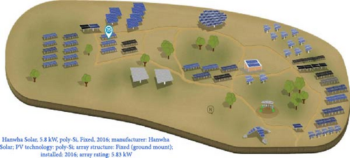
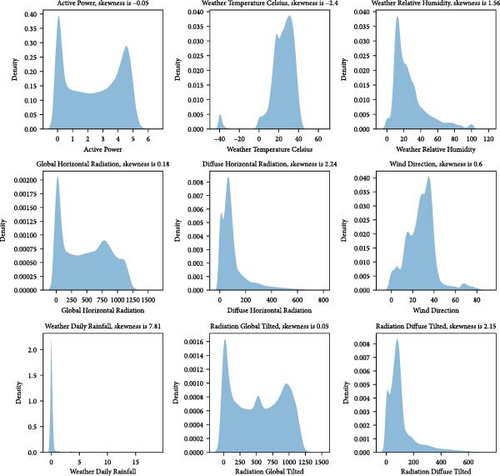
Table 1 provides an illustration of the attributes’ description, and Figure 2 shows the distribution of meteorological data.
| Feature names | Column no. | Type | Minimum/maximum | Mean | Missing | Missing (%) |
|---|---|---|---|---|---|---|
| Timestamp | 0 | Datetime | 2020-01-01 06:00:00/2020-12-31 19:00:00 | — | 0 | 0.0 |
| Active Power | 1 | Numerical | −0.004266666/6.0291996 | 2.434698 | 918 | 1.6 |
| Weather Temperature Celsius | 2 | Numerical | −39.987949/61.371174 | 23.44262 | 9 | <0.1 |
| Weather Relative Humidity | 3 | Numerical | 0/115.43026 | 26.89988 | 9 | <0.1 |
| Global Horizontal Radiation | 4 | Numerical | 0/1524.5419 | 483.6441 | 10 | <0.1 |
| Diffuse Horizontal Radiation | 5 | Numerical | 0/769.85999 | 99.91580 | 10 | <0.1 |
| Wind Direction | 6 | Numerical | −4.623755/87.849037 | 27.88489 | 7 | <0.1 |
| Weather Daily Rainfall | 7 | Numerical | 0/18.399998 | 0.249013 | 4 | <0.1 |
| Radiation Global Tilted | 8 | Numerical | 0.12903146/1408.8971 | 528.6797 | 2226 | 3.9 |
| Radiation Diffuse Tilted | 9 | Numerical | 0.11463284/723.46216 | 106.9393 | 2226 | 3.9 |
3. Methodology and the Proposed Approach
3.1. Regression Analysis Techniques
ML regression analysis is a predictive modeling technique used to understand the relationship between a dependent variable (often referred to as the target or output) and one or more independent variables (also known as features or inputs). The primary goal is to predict continuous values, as opposed to discrete labels, which are the focus of classification tasks. This analysis method is commonly employed across various fields, including sales forecasting, stock price estimation, credit scoring, and energy consumption prediction (e.g., forecasting energy usage in buildings or industrial processes). Regression analysis in ML comes in various forms, with the choice of method depending on the specific nature of the data.
There are various regression methods such as linear regression, ridge regression, Least Absolute Shrinkage and Selection Operator (LASSO) regression, Elastic Net, Extra Trees Regressor, random forest regressor, GB regressor, and XGBoost Regressor. To address of how these model process the used meteorological data for solar power prediction, the main steps can be summarized as follows:
Step 1. Data collection: Meteorological data (e.g., solar radiation, temperature, humidity, and wind speed) and the corresponding solar power output data are collected.
Step 2. Data preprocessing: Missing values are handled, outliers are removed, and any errors in the data are corrected. Also, features are normalized to ensure they are on a similar scale, which is particularly important for methods sensitive to feature scales.
Step 3. Feature selection process: The most relevant features for the model are identified and selected. Then, the raw data are transformed into meaningful features to improve model performance. In this step, various feature selection techniques are discussed such as PC, VIF, MI, SFS, BE, RFE, and EM. A general overview of the steps involved in applying feature selection techniques to identify the most influential factors for PV power prediction can be described as follows:
- •
Correlation analysis: PC is used to assess the linear relationships between each feature and the PV power output. Also, VIF is computed to detect multicollinearity and remove or combine features with high VIF values.
- •
MI: The MI between each feature and the PV power output is calculated to measure the nonlinear dependency. Then, the features are ranked based on their MI scores and select the most relevant ones.
- •
SFS: It starts with no features and iteratively adds features that improve model performance the most. Then, the model performance is evaluated at each step using cross-validation or a performance metric.
- •
BE: It starts with all features and iteratively removes the least significant feature based on model performance. Then, metrics like p-values or feature importance scores are utilized to decide which features to remove.
- •
RFE: The model is trained with all features, and they are ranked based on their importance. The least important features are iteratively removed, and the model is retrained until the desired number of features is reached.
- •
EM: LASSO regression or tree-based models like random forests or XGBoost models are incorporated as part of the training process. Then, the feature importance directly from these models is selected.
Step 3.2. Evaluate the selected features: After utilizing various feature selection methods, each generates a set of selected features. These sets are then tested using a random forest regressor model, and the prediction accuracy is compared across the different methods (the results are tabulated and compared in Table 2).
| Method | No. of selected features | RMSE | R2 |
|---|---|---|---|
| PC | 5 | 0.166435 | 0.991222 |
| VIF | 4 | 0.192499 | 0.988257 |
| MI | 5 | 0.158889 | 0.992000 |
| SFS | 5 | 0.160618 | 0.991825 |
| BE | 6 | 0.164447 | 0.991430 |
| RFE | 4 | 0.168400 | 0.991014 |
| EM | 2 | 0.182029 | 0.989500 |
- Abbreviations: BE, backward elimination; EM, embedded method; MI, mutual information; PC, Pearson correlation; RFE, recursive feature elimination; RMSE, root mean square error; SFS, step forward selection; VIF, variance inflation factor.
Step 3.3. Finalize feature set: Based on the evaluation results, the feature selection methods that yield the highest accuracy are chosen, and their selected features are compared to identify common ones. A threshold value of 1 is used, so features selected by more than one method are considered, with these common features designated as primary features.
Step 4. Model training: The data are divided into training and test sets to assess model performance. Then, the chosen regression model is implemented to fit the training data, using the selected primary features to predict solar power output.
Step 5. Model evaluation: The trained model is evaluated on the test set to check its performance on unseen data. Also, the metrics of RMSE, mean absolute error (MAE), and R2 are evaluated to assess accuracy.
Step 6. Prediction: The trained model is utilized to predict solar power output based on new or future meteorological data.
These steps provide a structured approach to utilizing meteorological data for solar power prediction, regardless of the specific regression technique used.
3.1.1. Linear Regression
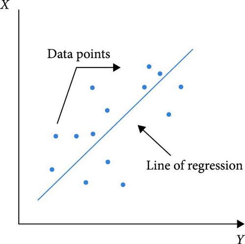
In this case, X serves as the explanatory variable, and Y represents the dependent variable. The value of Y at X = 0 is the intercept, and the slope of the line is b. The least squares approach is the most popular strategy to determine a regression line [39]. This calculates the best line for data. It minimizes vertical distances squared from each point to line. Figure 3 shows an example of linear regression line and some data points.
3.1.2. Ridge Regression
This is a standard, multiple-variable linear regression equation. In this case, X is any predictor (independent variable), B is the regression coefficient associated with that independent variable, Y is the expected value (dependent variable), and X0 is the value of the dependent variable (also known as the Y-intercept) when the independent variable equals zero.
3.1.3. LASSO Regression
L1 regularization, another name for LASSO regression, is a widely used method in ML and statistical modeling that estimates and predicts the associations between variables [41]. LASSO regression makes predictions more accurate by shrinking data values. It shrinks the values toward a central point like the mean. This helps the model make better predictions by reducing errors.
Because LASSO regression can automatically choose variables, it is perfect for predictive problems as it can simplify models and improve prediction accuracy [40]. However, because LASSO regression generates more bias by decreasing coefficients toward zero, ridge regression might perform better than LASSO regression. Because it picks a feature at random to include in the model, it also has issues with linked features in the data.
3.1.4. Elastic Net Regression
Elastic Net regression combines the best aspects of ridge and LASSO regression [42]. Elastic Net is a hybrid of LASSO and ridge, the two most often used regularized forms of linear regression. While LASSO uses an L1 penalty, ridge uses an L2 penalty. Elastic Net utilizes both the L2 and the L1 penalty, so you do not have to pick between these two models [42].
Elastic Net regression is used to deal with the problems of multicollinearity and overfitting, which are frequently seen in high-dimensional datasets. Comparing Elastic Net regression to LASSO and ridge regression, there are a number of benefits. For choosing features, Elastic Net performs feature selection, which facilitates model interpretation. It manages multicollinearity between variables by grouping them, which can be very useful in certain datasets. Finally, it balances ridge and LASSO regression to handle the bias-variance trade-off.
3.1.5. Extra Trees Regressor
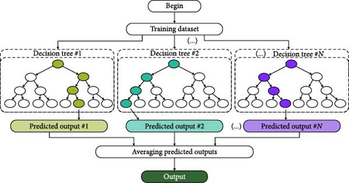
Extra Trees (short for excessively randomized trees) Regressor is an ensemble supervised ML method that employs decision trees [43]. The additional trees algorithm, like the random forest approach, creates a huge number of decision trees, but it does so randomly and without replacement for each tree.
This creates a dataset where each tree has a unique sample. In addition, a certain set of features are chosen at random for each tree. The most significant and unique characteristic of Extra Trees is the random selection of a splitting value for a feature. Instead of splitting the data and determining a locally optimum value using entropy or Gini, the method selects a split value at random. The trees become diverse and uncorrelated as a result. Random forest is slower than this technique. A simplified representation of the Extra Trees approach regression procedure is presented in Figure 4.
3.1.6. Random Forest Regressor
It is an algorithm for supervised learning that provides regression using an ensemble learning technique. It is not a boosting approach; rather, it is a bagging technique [44]. Since the trees in random forests grow in parallel, there is no contact between them as they are growing. The random forests algorithm makes its final forecast by averaging the predictions of several decision trees that were trained on a dataset with a real tree structure.
Since the random forests algorithm performs well with high-dimensional data, missing values, and outliers, they are regarded as strong and powerful ML models. They also do not require a lot of hyperparameter tweaking and are comparatively simple to utilize.
3.1.7. GB Regressor
GB has become a popular ML technique for issues involving regression and classification. Several weak learners are combined into one stronger model using this ensemble learning technique [45, 46]. GB’s primary concept is to repeatedly add new, vulnerable learners to the model while training each one to fix the errors created by the prior ones [47]. Decision trees are commonly used in GB [48]. The loss function is commonly used as the objective function for GB classifiers, quantifying the difference between the expected and actual output. GB is a very useful technique for addressing missing data, outliers, and huge cardinality categories on the features with no requiring further processing. It is capable of detecting any nonlinear relationship that exists between the features and the model target.
3.1.8. XGBoost Regressor
XGBoost, or eXtreme GB, is a ML technique that is a part of the GB framework, which is a subset of ensemble learning. It makes use of regularization techniques to improve model generalization using decision trees as foundation learners. XGBoost is a popular choice for computationally demanding tasks including regression and classification due to its proficiency in feature importance analysis, management of missing information, and computational economy [49]. XGBoost creates a predictive model by repeatedly integrating the predictions of several different models, most frequently decision trees. The way the algorithm operates is by gradually adding weak learners to the ensemble, with each new learner concentrating on fixing any errors produced by the previous ones. During training, it minimizes a predetermined loss function using the gradient descent optimization method. The capacity to manage complicated relationships in data, regularization strategies to avoid overfitting, and the use of parallel processing for effective computing are some of the main characteristics of the XGBoost algorithm [50]. XGBoost is frequently employed in several domains due to its great prediction performance and adaptability across multiple datasets.
3.2. Feature Selection Techniques
Feature selection is a fundamental concept in ML that significantly impacts model performance. It involves identifying and selecting the most relevant features (or variables) from a dataset that contribute to the predictive power of a ML model. The primary goal of feature selection is to enhance model performance by reducing overfitting, improving accuracy, and decreasing training time. Feature selection techniques can be broadly categorized into three types: filter methods, wrapper methods, and EMs [51]. The choice of technique depends on the nature of the data, the type of model being used, and the specific goals of the analysis. Filter methods are fast and straightforward but may not capture complex feature interactions, wrapper methods are more accurate but computationally intensive, and EMs strike a balance by integrating feature selection directly into the model training process.
3.2.1. Filter Methods
Using this strategy, only the relevant feature subset is taken and filtered. Once the features are chosen, the model is constructed. In this research paper, filtering is carried out using PC, VIF, and MI which are the most widely used methods.
3.2.1.1. PC
3.2.1.2. VIF
3.2.1.3. MI
The joint probability mass function of X and Y is denoted by p (x, y), whereas the marginal probability mass functions of X and Y are represented by p (x) and p (y), correspondingly.
3.2.2. Wrapper Methods
They require a single ML algorithm, and its assessment criteria are based on its performance. Feed the features to the chosen ML algorithm, and then add or remove features according to the model’s performance. Even though it requires a greater amount of computing power and is an iterative process, the accuracy is higher than with the filter methods [51].
3.2.2.1. SFS
The iterative process of forward selection with no features in the model is firstly considered. Then, adding the feature is continued that best enhances the model with each iteration till the performance of the model is no longer improved by the addition of a new variable.
3.2.2.2. BE
BE is a technique that enhances model performance by starting with all features and eliminating the least important feature at each iteration. It is kept implemented until there is no discernible improvement in the features removed.
3.2.2.3. RFE
The approach of feature selection known as RFE involves fitting a model and eliminating the weakest feature or features until the desired number of features is attained.
3.2.3. EM
Although filter methods are computationally efficient, they completely disregard the learning algorithm’s biases. Wrapper methods yield greater prediction accuracy estimates than filter methods because they account for the biases in the learning methods. Wrapper methods, however, require a significant amount of computing power. By incorporating the feature selection into the model building process, EMs provide a trade-off between the two methods [51].
Using EMs, features that are most helpful to the training for a given iteration are extracted through an iterative process. LASSO regularization and other regularization techniques are the most used embedded algorithms that penalize a feature given a coefficient threshold. LASSO penalizes a feature’s coefficient and sets it to zero if it is unimportant. The features having a coefficient of zero are removed to take the remaining ones.
3.3. Proposed Approach
This part covers the general procedures of the suggested model, the feature selection method, and the key performance measures that are utilized to assess the suggested model’s efficacy.
3.3.1. Overview of the Proposed Model
Figure 5 provides an overview of the proposed model.
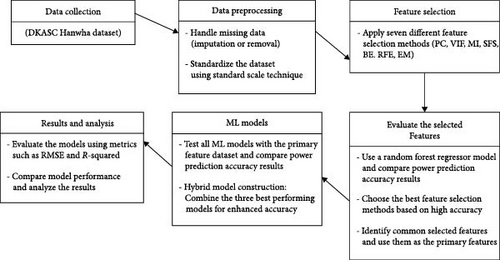
The dataset is then split into two categories: testing and training, wherein 70% of the data are used for the training phase and the remaining 30% are used for testing. To solve the overfitting problem, seven different feature selection methods PC, VIF, MI, SFS, BE, RFE, and EM are considered in order to choose the most relevant features and address the overfitting issue.
3.3.2. Feature Selection
The DKASC Hanwha Solar dataset comprises 10 columns, as detailed in Section 2. Columns 2 through nine contain meteorological data, which includes eight features that we need to analyze carefully to select only the most important ones for maximizing power prediction accuracy. We employ various feature selection methods, generating a set of selected features for each method. Each set of selected features is tested using a random forest regressor model, and the accuracy of power predictions is compared across methods. The feature selection methods that yield the highest accuracy are chosen, and the sets of selected features are then compared to identify common features, which are designated as primary features. Utilizing these most relevant features can enhance model performance by focusing on the most informative data.
The primary features used by ML models are constructed based on the list of selected features based on seven different techniques: PC, VIF, MI, SFS, BE, RFE, and EM. A robust strategy is to test models using alternative ways to choose features (and quantities of features) and choose the one that yields a model having the greatest efficiency. There are actually numerous methods to rate features and choose features according to these scores. Compared to linear regression, random forest is a robust ML technique that may produce superior outcomes. It consists of a group of decision trees, which are far more effective than linear models at capturing nonlinear correlations between data and goal variables. This section will compare various models constructed from features chosen using the seven distinct ways to an evaluation of a random forest regressor model with all features.
Figure 6 displays the heatmap regarding the PC coefficient, to assess how linear the relationship is between two variables. In this map, darker colors indicate strong positive correlations, while lighter colors indicate strong negative correlations.
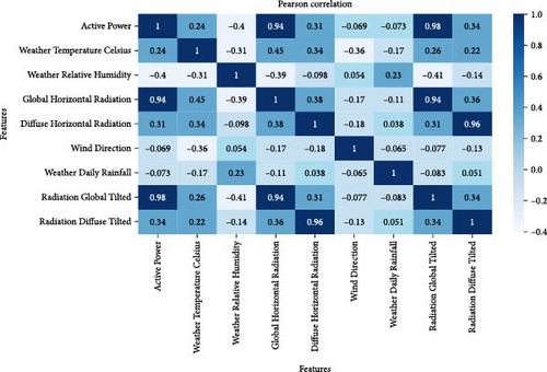
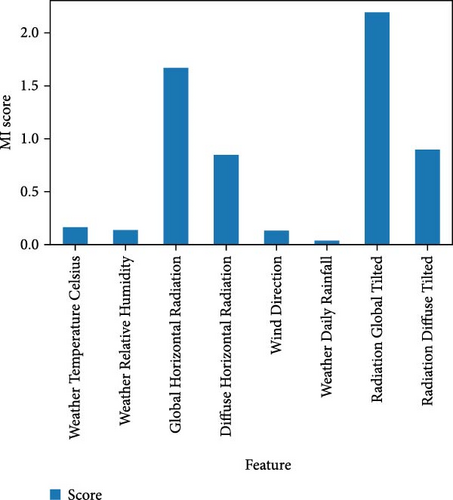
As seen in Figure 6, the PC coefficient heatmap provides a more understandable representation of the dependency between variables. From PC heatmap, Weather Relative Humidity, Global Horizontal Radiation, Diffuse Horizontal Radiation, Radiation Global Tilted, and Radiation Diffuse Tilted based on the degree of association are chosen. Additionally, the VIF is utilized as a measure to determine the degree of multicollinearity among multiple regression variables. The following features were chosen using VIF: Radiation Global Tilted, Weather Daily Rainfall, Diffuse Horizontal Radiation, and Weather Relative Humidity. Also, MI is utilized to measure how much knowing one thing helps reduce the uncertainty about the other. It is a way to quantify the connection between two quantities. Data visualization is a great follow-up to utility ranking. Figure 7 illustrates the MI score, and features with a high score are selected. Radiation Global Tilted, Global Horizontal Radiation, Radiation Diffuse Tilted, Diffuse Horizontal Radiation, and Weather Temperature Celsius are the features that have been chosen.
Moreover, Weather Temperature Celsius, Weather Relative Humidity, Global Horizontal Radiation, Radiation Global Tilted, and Radiation Diffuse Tilted are the features that were chosen using the SFS technique. The following features were chosen using the BE technique: Wind Direction, Global Horizontal Radiation, Weather Temperature Celsius, Weather Relative Humidity, Daily Rainfall, and Radiation Global Tilted. The features selected by RFE technique are Weather Relative Humidity, Global Horizontal Radiation, Radiation Global Tilted, and Radiation Diffuse Tilted. There are two features only selected by EM technique, Global Horizontal Radiation, and Radiation Global Tilted. Finally, Table 3 displays the selected features for each feature selection method. By examining the selection counts, we can identify the common features that were selected across different methods.
| Method | Column number/features | No. of selected features for each method | |||||||
|---|---|---|---|---|---|---|---|---|---|
| 2 | 3 | 4 | 5 | 6 | 7 | 8 | 9 | ||
| PC | — | √ | √ | √ | — | — | √ | √ | 5 |
| VIF | — | √ | — | √ | — | √ | √ | — | 4 |
| MI | √ | — | √ | √ | — | — | √ | √ | 5 |
| SFS | √ | √ | √ | — | — | — | √ | √ | 5 |
| BE | √ | √ | √ | — | √ | √ | √ | — | 6 |
| RFE | — | √ | √ | — | — | — | √ | √ | 4 |
| EM | — | — | √ | — | — | — | √ | — | 2 |
| Selection count | 3 | 5 | 6 | 3 | 1 | 2 | 7 | 4 | |
- Abbreviations: BE, backward elimination; EM, embedded method; MI, mutual information; PC, Pearson correlation; RFE, recursive feature elimination; SFS, step forward selection; VIF, variance inflation factor.
The table provides a comprehensive overview of features selected by various feature selection methods for PV power prediction. It reveals that Global Horizontal Radiation and Radiation Global Tilted are consistently identified across most methods, underscoring their significant influence on PV power output. These features are selected by seven and six methods, respectively, indicating their robust relevance. Weather Temperature Celsius, Weather Relative Humidity, and Radiation Diffuse Tilted also appear frequently, suggesting they contribute importantly but with less consistency across methods. Notably, BE is the most inclusive, selecting six features, including additional ones like Wind Direction and Daily Rainfall, which are not chosen by other methods. This broad selection indicates BE’s tendency to retain a larger set of features before eliminating them. In contrast, the EM is the most selective, choosing only two features, reflecting its focus on the most impactful variables. The Selection Count shows that while Global Horizontal Radiation stands out with the highest frequency, features like Weather Temperature Celsius and Weather Relative Humidity have moderate counts, highlighting their variable importance.
We then test the selected features from each feature selection method using a random forest regressor model and compare the results. Table 2 presents the outcomes for the final selected features.
The results in Table 2 reveal the impact of different feature selection techniques on the performance of regression models, assessed through RMSE and R2 metrics. Among the techniques, MI exhibits the most impressive performance, with the lowest RMSE of 0.158889 and the highest R2 of 0.992000. This suggests that the features selected by MI provide the most accurate and explanatory model. SFS and PC analysis also deliver robust results, with SFS achieving an RMSE of 0.160618 and R2 of 0.991825, and PC analysis yielding an RMSE of 0. 166435 and R2 of 0.991222. These techniques effectively balance the number of features with model performance, ensuring that critical information is retained without unnecessary complexity.
Conversely, the EM selects only two features, resulting in the highest RMSE of 0.182029 and the lowest R2 of 0.989500 among the methods. This indicates that while fewer features simplify the model, they may also omit essential information, reducing predictive accuracy and explanatory power. Similarly, the VIF and RFE techniques, which select four features each, show moderately lower performance metrics. VIF’s RMSE is 0.192499 with an R2 of 0.988257, while RFE’s RMSE is 0.168400 with an R2 of 0.991014, suggesting that these methods might exclude some informative features or introduce redundancy.
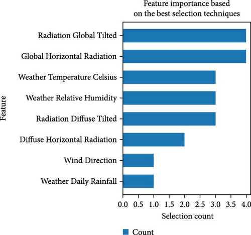
In this study, PC, MI, SFS, and BE based on RMSE values are selected and implemented to draw the following figure to describe the features importance. Figure 8 illustrates the importance of various features as determined by the selected feature selection techniques. Table 4 displays the features selected by the PC, MI, SFS, and BE methods, with the selection count used to assess and describe feature importance.
| Method | Column number/features | |||||||
|---|---|---|---|---|---|---|---|---|
| 2 | 3 | 4 | 5 | 6 | 7 | 8 | 9 | |
| PC | — | √ | √ | √ | — | — | √ | √ |
| MI | √ | — | √ | √ | — | — | √ | √ |
| SFS | √ | √ | √ | — | — | — | √ | √ |
| BE | √ | √ | √ | — | √ | √ | √ | — |
| Selection count | 3 | 3 | 4 | 2 | 1 | 1 | 4 | 3 |
- Abbreviations: BE, backward elimination; MI, mutual information; PC, Pearson correlation; SFS, step forward selection.
After this assessment, the features are filtered to retain only those with an information gain above a specific threshold. This threshold was determined through extensive experimentation to maximize prediction accuracy, ultimately setting the threshold at 1. Consequently, features selected by more than one method are considered. The final input features, designated as Primary Features, include Radiation Global Titled, Global Horizontal Radiation, Weather Temperature Celsius, Weather Relative Humidity, Radiation Diffuse Titled, and Diffuse Horizontal Radiation.
3.3.3. Regression Models
After identifying the most relevant features through feature selection methods, the less important and irrelevant features were eliminated. This process refined the dataset, reducing it to seven columns: six columns corresponding to the key meteorological variables (the input features) and one column representing the PV power output, which serves as the prediction target.
Next, data standardization was performed to ensure that all features were on the same scale and range, preventing any single feature from disproportionately influencing the model’s predictions. This step was essential for improving the accuracy and performance of many ML algorithms, especially those sensitive to feature scaling. Standardization also involved correcting any data inconsistencies and handling outliers, thereby improving the overall quality and reliability of the dataset. Table 5 provides a snapshot of the dataset after the standardization process. The data presented includes 10 randomly selected rows, showcasing the standardized values for each of the six key features.
| Row index | Diffuse Horizontal Radiation | Global Horizontal Radiation | Radiation Diffuse Tilted | Radiation Global Tilted | Weather Relative Humidity | Weather Temperature Celsius |
|---|---|---|---|---|---|---|
| 498 | −0.024379 | 1.440419 | −0.191172 | 1.294711 | −0.531889 | 0.235946 |
| 2996 | −0.972909 | −1.256791 | −0.296669 | 1.367570 | −1.187329 | −3.243804 |
| 1023 | 3.622827 | 0.999440 | 3.583228 | 0.892936 | −0.731438 | 0.602466 |
| 5050 | −0.969549 | −1.254162 | 1.272719 | −0.301553 | −1.266024 | −3.314420 |
| 3645 | −0.966517 | −1.255915 | 1.779339 | 1.001072 | −1.354223 | −3.394903 |
| 4750 | 0.120411 | 1.457192 | −0.055305 | 1.312147 | −0.712017 | 0.734318 |
| 1132 | 0.409328 | −0.808236 | 0.322156 | −0.963642 | 2.998456 | 0.069261 |
| 5324 | −0.925316 | −1.244115 | 0.432101 | −0.968838 | −1.367583 | −3.407290 |
| 4021 | −0.400967 | −0.097872 | −0.529834 | −0.335821 | −0.868302 | 0.487791 |
| 740 | −0.495449 | −0.139009 | −0.600254 | −0.251373 | 0.684165 | −0.050749 |
After the standardization process, the dataset was randomly split into two subsets: 70% of the data was allocated for training, and the remaining 30% was set aside for testing. This split ensures that the model can learn from the majority of the data while being evaluated on unseen data to assess its generalization capability. The primary goal of the model is to analyze the numerical meteorological data (such as temperature, radiation, and humidity) and establish patterns or relationships between these variables and the electrical energy generated by solar cells. Once these relationships are identified, the model can predict the energy output based on new meteorological data, even if it has not encountered those specific inputs during training.
In this study, scikit-learn’s prebuilt estimators (open-source Python library for ML models [56, 57]) were used which provides a comprehensive set of tools for both supervised and unsupervised learning. Each estimator is trained on the data using its fit method. The input to the fit method is the sample matrix X (which includes the meteorological features, where each row represents an individual observation and each column represents a feature), and the target values Y, which correspond to the actual PV power output. Once trained, the estimator can predict target values for new, unseen data, based on the learned patterns from the training data. In this study, the sample matrix includes six columns representing the primary features, with the target variable being the generated electrical energy. The estimator is trained using 70% of the data. Once trained, the estimator can predict target values for new input data without requiring retraining.
Following training, the model was tested using the remaining 30% of the dataset. The new data matrix (X) was input into the model, and the resulting predicted values (Y) were compared with actual values to assess prediction error. Table 6 shows the predicted and original data for 10 randomly selected samples when training and testing the linear regression model used from the scikit-learn library.
| Row index | Actual PV power | Predicted PV power |
|---|---|---|
| 3956 | 4.906299 | 4.918425 |
| 867 | 4.127600 | 4.226289 |
| 1414 | 0.995533 | 0.942023 |
| 2840 | 4.750800 | 4.755520 |
| 4870 | 1.360933 | 1.381778 |
| 1162 | 2.667434 | 2.668501 |
| 324 | 4.048267 | 4.122180 |
| 831 | 1.075600 | 1.244946 |
| 1333 | 3.521366 | 3.546563 |
| 2014 | 4.638200 | 4.648940 |
- Abbreviation: PV, photovoltaic.
This research also leverages multiple ML models from the scikit-learn library, including ridge regression, LASSO Regression, Elastic Net, Extra Trees Regressor, random forest regressor, and GB regressor. Each of these models is trained on 70% of the dataset, just like the linear regression model, allowing them to learn the patterns between the key meteorological features and the generated PV power. After training, the models are tested on the remaining 30% of the data to evaluate their performance on unseen data. For each model, the prediction process involves taking the test set input (which includes the meteorological features) and generating predicted values for the PV power output. These predicted values are then compared with the actual values to assess how well each model performs. The tables (Tables 7–12) present a random sample of predicted PV power values for each of the models used, highlighting their performance on individual test samples.
| Row index | Actual PV power | Predicted PV power |
|---|---|---|
| 852 | 1.065667 | 1.344560 |
| 3651 | 0.088667 | 0.160171 |
| 4111 | 1.380267 | 1.699295 |
| 1237 | 4.433100 | 4.103973 |
| 307 | 1.076400 | 1.484775 |
| 107 | 0.183467 | 0.210443 |
| 2925 | 0.000000 | 0.054042 |
| 5181 | 2.684367 | 2.515708 |
| 3180 | 2.754433 | 2.545339 |
| 4429 | 4.131333 | 4.207422 |
- Abbreviation: PV, photovoltaic.
| Row index | Actual PV power | Predicted PV power |
|---|---|---|
| 1699 | 1.934400 | 1.629623 |
| 3529 | 0.583133 | 0.454784 |
| 722 | 4.142833 | 4.298744 |
| 840 | 3.989933 | 3.800298 |
| 4514 | 1.711667 | 1.738500 |
| 3897 | 0.000000 | 0.811547 |
| 5358 | 0.000000 | 0.053930 |
| 2020 | 1.610000 | 1.622825 |
| 4830 | 4.713334 | 4.917562 |
| 2104 | 4.046600 | 4.126561 |
- Abbreviations: LASSO, Least Absolute Shrinkage and Selection Operator; PV, photovoltaic.
| Row index | Actual PV power | Predicted PV power |
|---|---|---|
| 206 | 0.009067 | −0.014759 |
| 3418 | 3.448400 | 3.478625 |
| 3395 | 4.879633 | 5.030806 |
| 4220 | 0.743067 | 0.662497 |
| 1119 | 3.808200 | 3.632128 |
| 4493 | 4.169366 | 4.029801 |
| 72 | 4.483334 | 4.788738 |
| 1046 | 2.856467 | 2.687984 |
| 4757 | 0.000000 | 0.063725 |
| 2161 | 3.260300 | 3.127507 |
- Abbreviation: PV, photovoltaic.
| Row index | Actual PV power | Predicted PV power |
|---|---|---|
| 402 | 4.880700 | 4.827788 |
| 1345 | 0.860333 | 0.822132 |
| 1807 | 3.062900 | 3.110857 |
| 2470 | 4.976267 | 4.989662 |
| 1950 | 2.564233 | 2.582682 |
| 3403 | 4.422999 | 4.522958 |
| 2306 | 2.747400 | 2.775152 |
| 3512 | 0.105500 | 0.101361 |
| 2198 | 0.014067 | 0.016680 |
| 4108 | 4.490734 | 4.502964 |
- Abbreviation: PV, photovoltaic.
| Row index | Actual PV power | Predicted PV power |
|---|---|---|
| 3778 | 3.098900 | 3.111685 |
| 3833 | 2.495766 | 2.516712 |
| 3391 | 3.707500 | 3.720703 |
| 3994 | 0.866733 | 0.836290 |
| 5346 | 0.212933 | 0.180451 |
| 277 | 3.789867 | 3.873528 |
| 3035 | 5.033367 | 5.063702 |
| 2751 | 0.000000 | 0.000000 |
| 4430 | 5.194300 | 4.765915 |
| 210 | 2.027300 | 2.014854 |
- Abbreviation: PV, photovoltaic.
| Row index | Actual PV power | Predicted PV power |
|---|---|---|
| 668 | 4.780767 | 4.911787 |
| 5273 | 4.740500 | 4.692913 |
| 752 | 5.055233 | 5.053923 |
| 3244 | 3.388200 | 3.609603 |
| 2874 | 0.000000 | 0.001427 |
| 2563 | 2.226067 | 2.488140 |
| 4510 | 0.214533 | 0.149639 |
| 1910 | 3.673167 | 3.674817 |
| 321 | 4.610366 | 4.597660 |
| 4582 | 1.556167 | 1.649106 |
- Abbreviations: GB, gradient boosting; PV, photovoltaic.
The XGBoost library was employed to implement the XGBoost Regressor, a highly optimized GB tool designed for efficient and scalable ML model training. The model was trained on the designated training data and evaluated on the test set. Table 13 provides a random sample of PV power predictions made by it.
| Row index | Actual PV power | Predicted PV power |
|---|---|---|
| 4200 | 0.734000 | 0.748405 |
| 1221 | 4.255466 | 4.190846 |
| 3067 | 3.947300 | 3.963487 |
| 4067 | 3.661800 | 3.558964 |
| 5141 | 0.000000 | 0.017265 |
| 3123 | 4.576834 | 4.526834 |
| 5382 | 0.418500 | 0.388340 |
| 4756 | 5.104000 | 5.104790 |
| 2704 | 4.469967 | 4.434934 |
| 737 | 0.957767 | 0.872789 |
- Abbreviations: PV, photovoltaic; XGBoost, eXtreme Gradient Boosting.
3.3.4. Performance Measure Indices
A lower RMSE and MAE reflect greater prediction accuracy. Similarly, an R2 value approaching 1 indicates that the predictions are highly accurate [58]. There is always going to be a difference between the RMSE and MAE; the larger the gap, the more variance there is in the individual errors within the sample.
4. Results and Discussion
The models in this study were developed using Python on the Google Colab platform, leveraging several ML libraries, including Numpy, Pandas, and scikit-learn. The Google Colab environment utilized an AMD EPYC 7B12 processor (2250 MHz), 12.67 GB of RAM, and a Linux operating system. Initially, data preprocessing was performed, which involved cleaning the dataset by replacing all missing values with the most suitable estimates after thoroughly analyzing the dataset. Before applying ML algorithms, the data was standardized. Various feature selection methods, such as PC, VIF, MI, SFS, BE, RFE, and EM, were then applied to refine the dataset.
The dataset was split into training and testing sets with a 70:30 ratio, allocating 70% of the data (39,572 records) for training and 30% (16,960 records) for testing. Finally, both traditional and hybrid ML algorithms were implemented to evaluate the models’ performance including linear regression, ridge regression, LASSO regression, Elastic Net, Extra Trees Regressor, random forest regressor, GB regressor, XGBoost regressor, and hybrid model of XGBoost Regressor, Extra Trees Regressor, and GB regressor are applied to the dataset. The following table shows the results for all regression algorithms. The results indicate a clear trade-off between training time and model accuracy. While traditional linear models are extremely fast to train, they offer lower accuracy, as evidenced by their higher RMSE and lower R2 values. In contrast, more complex models like Extra Trees Regressor, random forest regressor, GB regressor, and XGBoost Regressor provide significantly better accuracy but require longer training times. The hybrid model, with its superior accuracy, reflects the effectiveness of combining multiple robust algorithms to capture intricate patterns in the data, albeit at a higher computational cost.
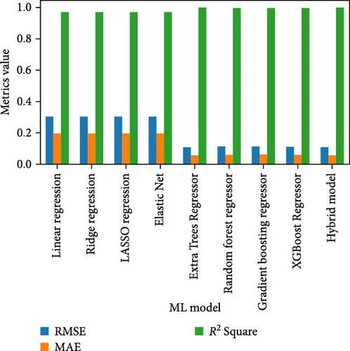
Table 14 showcases the performance of various traditional and hybrid ML algorithms applied to a dataset, evaluated using metrics such as training time, RMSE, MAE, and R2. Linear, ridge, LASSO regressions, and Elastic Net exhibit the shortest training times, with ridge regression being the fastest at 0.000590 s. These models yield similar performance metrics, with RMSE values around 0.305 and R2 values near 0.970. The MAE values are also close, around 0.196, indicating consistent but moderate predictive accuracy. Despite their rapid training times, these models are less accurate compared to more complex algorithms, making them suitable for scenarios where speed is more critical than precision. On the other side, ensemble methods such as Extra Trees Regressor, random forest regressor, and GB regressor demonstrate significantly improved performance over linear models. Extra Trees Regressor, for instance, achieves an RMSE of 0.109884 and an R2 of 0.996156, with an MAE of 0.056846. Random forest regressor and GB regressor also perform well, with RMSE values of 0.116084 and 0.114795, respectively, and corresponding R2 values above 0.995. These models, however, require longer training times, reflecting their complexity and computational demands. Moreover, XGBoost Regressor stands out with a strong performance, achieving an RMSE of 0.111622 and an R2 of 0.996034, coupled with a relatively short training time of 1.574913 s. This balance of accuracy and efficiency makes XGBoost Regressor a robust choice for many applications. The hybrid model, which combines XGBoost Regressor, Extra Trees Regressor, and GB regressor, achieves the best overall results with the lowest RMSE of 0.108735 and the highest R2 of 0.996228. The MAE of 0.058998 further underscores its exceptional accuracy. However, the hybrid model has the longest training time at 144.4991 s, indicating the high computational cost of integrating multiple algorithms.
| Method | Training time (s) | RMSE | MAE | R2 |
|---|---|---|---|---|
| Linear regression | 0.003471 | 0.305010 | 0.195990 | 0.970385 |
| Ridge regression | 0.000590 | 0.305010 | 0.196113 | 0.970385 |
| LASSO regression | 0.000715 | 0.305019 | 0.195787 | 0.970383 |
| Elastic Net | 0.403472 | 0.305024 | 0.195807 | 0.970382 |
| Extra Trees Regressor | 49.17437 | 0.109884 | 0.056846 | 0.996156 |
| Random forest regressor | 31.54947 | 0.116084 | 0.059530 | 0.995710 |
| GB regressor | 93.42595 | 0.114795 | 0.064757 | 0.995805 |
| XGBoost Regressor | 1.574913 | 0.111622 | 0.061950 | 0.996034 |
| Hybrid model | 144.4991 | 0.108735 | 0.058998 | 0.996228 |
- Abbreviations: GB, gradient boosting; LASSO, Least Absolute Shrinkage and Selection Operator; MAE, mean absolute error; RMSE, root mean square error; XGBoost, eXtreme Gradient Boosting.
Figure 9 contrasts predicted and actual values. If the model is well-fitted, the data points will be firmly grouped along the diagonal line. This shows that the actual and predicted values are closely related. In this plot, the data points are closely spaced along the diagonal, which suggests that the hybrid model’s predictions are accurate and consistent.
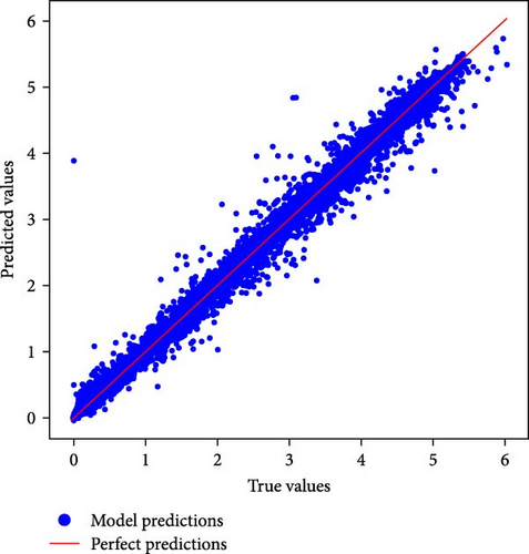
Figure 10 describes the relationship between the error values and its density. XGBoost Regressor, Extra Trees Regressor, and GB regressor for hybrid model based on the result they achieve are selected.
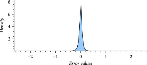
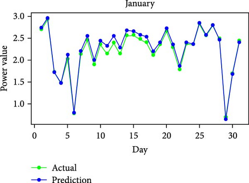
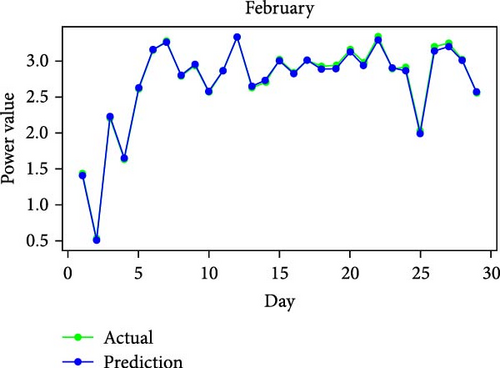
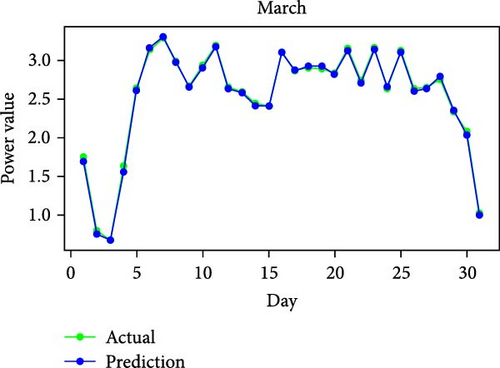
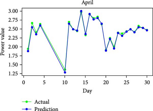
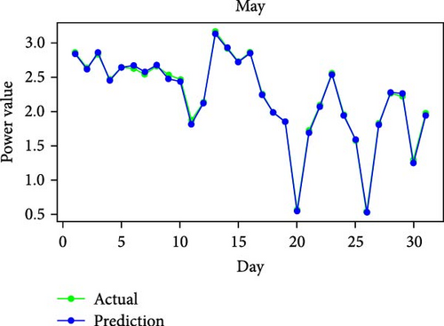
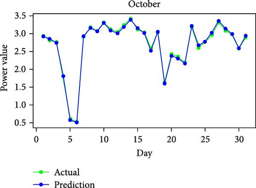
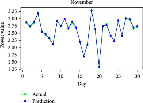
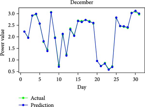
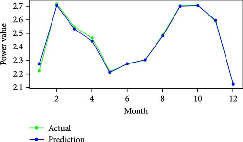
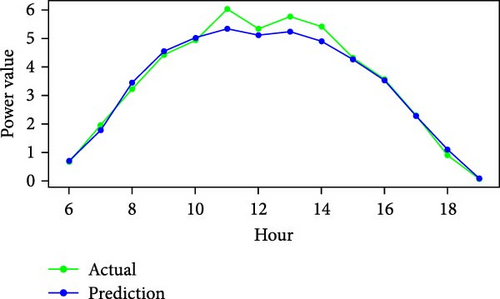
Figure 11 shows RMSE, R2, and MAE values for algorithms. Both RMSE and R2 are metrics used to evaluate the fit of a linear regression model to a dataset. RMSE measures the model’s predictive accuracy by quantifying the absolute difference between observed and predicted values of the response variable. In contrast, R2 assesses how well the predictor variables account for the variability in the response variable. In addition, Figure 12 displays the average generated and predicted power per day for every month of the year while Figure 13 illustrates the average actual and prediction power per month, and Figure 14 shows the maximum value for actual and prediction power for every hour for December.
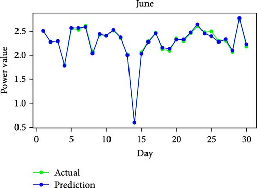
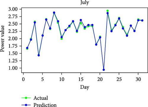
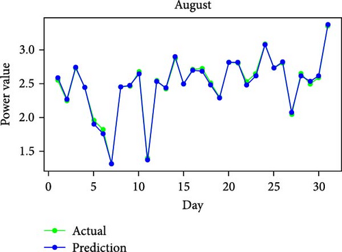
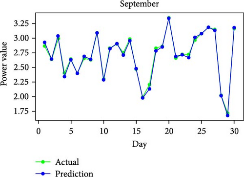
The dataset of 361 days in a year was divided into three categories of comparable day samples: sunny, cloudy, and rainy using Gaussian mixture model (GMM) [59]. Identical days were identified for the raw PV power samples using the GMM clustering technique, as described in [58]. Table 15 shows some samples clustering of sunny, cloudy, and rainy days. In particular, there were 62 days with rain, 120 days with clouds, and 179 days with sunshine. As shown, the RMSE for the sunny days cluster, consisting of 179 days, was 0.079076, indicating high predictive accuracy. The R2 value of 0.998007 suggests that the model explains almost all the variance in the data, reflecting excellent model performance. The training time for this cluster was 70.663 s, which is relatively moderate compared to the unclustered dataset. For the cloudy day cluster, with 120 days, the outcomes showed an RMSE of 0.144806 and an R2 value of 0.992314. While these metrics indicate good predictive performance, they are slightly less impressive than those for the sunny days cluster. Also, the rainy day cluster, encompassing 62 days, had an RMSE of 0.086474 and an R2 value of 0.997731. This cluster also shows high predictive accuracy, with performance metrics close to those of the sunny days cluster. Finally, the unclustered dataset of 361 days had an RMSE of 0.108735 and an R2 of 0.996228. The training time was the highest at 144.499 s. These results show that clustering the data into sunny, cloudy, and rainy categories improves predictive accuracy and reduces training time. The unclustered dataset’s higher RMSE suggests that treating all weather conditions uniformly introduces more variability and prediction errors, which clustering helps to mitigate.
| Dataset | Days | RMSE | R2 | Training time (s) |
|---|---|---|---|---|
| Sunny (clustered) | 179 | 0.079076 | 0.998007 | 70.663 |
| Cloudy (clustered) | 120 | 0.144806 | 0.992314 | 47.044 |
| Rainy (clustered) | 62 | 0.086474 | 0.997731 | 25.202 |
| Weather unclustered | 361 | 0.108735 | 0.996228 | 144.499 |
- Abbreviation: RMSE, root mean square error.
In order to illustrate how the suggested model outperforms conventional models in terms of prediction, several classical models are applied including LSTM, CNN, recurrent neural network (RNN), extreme learning machine (ELM), and QR and kernel density estimation deep learning networks (QRKDDNs) for comparison. Using the Rainy dataset as an example, each model is validated 10 times, and Table 16 displays the prediction results.
| Models | Training time | RMSE | R2 |
|---|---|---|---|
| QR-ELM [60] | 53 | 1.085463 | 0.825938 |
| QR-CNN [60] | 71 | 0.624928 | 0.874490 |
| QR-LSTM [28] | 118 | 0.874331 | 0.857201 |
| QR-RNN [61] | 137 | 0.562490 | 0.929510 |
| QRKDDN [58] | 154 | 0.301985 | 0.972064 |
| Proposed model | 25.202 | 0.086474 | 0.997731 |
- Abbreviations: CNNs, convolutional neural networks; ELM, extreme learning machine; LSTM, long short-term memory; QR, quantile regression; QRKDDNs, quantile regression and kernel density estimation deep learning networks; RNN, recurrent neural network.
From Table 16, the proposed model stands out with the lowest RMSE of 0.086474 and the highest R2 value of 0.997731, clearly outperforming all other models in terms of predictive accuracy. Additionally, it has the shortest training time at 25.202 s, showcasing its efficiency. The QR-ELM model has a training time of 53 s, which is more than double that of the proposed model. It records an RMSE of 1.085463 and an R2 value of 0.825938. These metrics indicate significantly lower accuracy, with the model explaining much less of the variance in the data compared to the proposed model. The QR-CNN model takes 71 s to train, yielding an RMSE of 0.624928 and an R2 of 0.874490. Although it performs better than the QR-ELM model, it still falls short of the proposed model in both prediction accuracy and efficiency. With a training time of 118 s, the QR-LSTM model achieves an RMSE of 0.874331 and an R2 value of 0.857201. This model requires significantly more time to train and yet offers less accurate predictions than the proposed model. The QR-RNN model has a training time of 137 s, an RMSE of 0.562490, and an R2 value of 0.929510. While its R2 value is higher than those of some other classical models, indicating better accuracy, it is still less efficient and accurate compared to the proposed model. The QRKDDN model, with a training time of 154 s, shows an RMSE of 0.301985 and an R2 value of 0.972064. Although this model performs better than the other classical models, it is still not as accurate or efficient as the proposed model. These results underscore the effectiveness of the proposed model, which not only predicts with greater accuracy but also does so more efficiently. This makes it particularly suitable for applications requiring real-time or near-real-time predictions, where both accuracy and speed are crucial. The comparative analysis confirms that the proposed model is a robust alternative to traditional approaches, offering substantial improvements in predictive performance and operational efficiency.
The model was set up and run 10 times to evaluate the computational efficiency of the proposed model with the comparative models used by the author [58] for the same data set. The comparative model’s schematic diagram and full description are included in the reference; however, they are not included in this study due to space limitations. Table 17 shows the average running time that resulted. The proposed model consistently demonstrates superior computational efficiency across all weather conditions. For sunny days, the proposed model has an average training time of 70.663 s, significantly lower than any of the comparative models. The QR-GRU model, the fastest among the comparatives, takes 187 s [58], which is more than double the time of the proposed model. On cloudy days, the proposed model again shows remarkable efficiency with an average training time of 47.044 s. The closest comparative model, QR-GRU, requires 166 s, while the QR-BiGRU takes 208 s [58]. The efficiency of the proposed model is most pronounced on rainy days, where it achieves an average training time of just 25.202 s. This is less than a quarter of the time needed by the QR-GRU model, which requires 108 s. The more complex QR-CNN-BiGRU and QR-CNN-BiLSTM-attention models take even longer, with training times of 151 and 204 s, respectively [58]. These results emphasize the proposed model’s advantage in computational efficiency without compromising predictive performance. The reduced training times make the proposed model ideal for real-time applications and scenarios where rapid retraining is necessary. This efficiency, combined with its previously demonstrated accuracy, positions the proposed model as a robust and practical solution in the field of predictive modeling.
| Models | Average training time (s) | ||
|---|---|---|---|
| Sunny | Cloudy | Rainy | |
| QR-GRU | 187 | 166 | 108 |
| QR-BiGRU | 236 | 208 | 124 |
| QR-BiGRU-attention | 249 | 215 | 128 |
| QR-CNN-BiGRU | 286 | 260 | 151 |
| QR-CNN-BiLSTM-attention | 463 | 334 | 204 |
| QRKDDN | 298 | 275 | 154 |
| Proposed model | 70.663 | 47.044 | 25.202 |
- Abbreviations: CNNs, convolutional neural networks; GRU, gated recurrent unit; LSTM, long short-term memory; QR, quantile regression; QRKDDNs, quantile regression and kernel density estimation deep learning networks.
5. Conclusion
In this paper, an accurate forecasting methodology is presented for the successful integration of renewable energy systems, particularly solar power generation. It introduces a pioneering hybrid predictive model framework that combines meteorological data, feature selection techniques, and multiple regression algorithms to enhance the accuracy of PV power prediction. The study is implemented on a PV system (Hanwha Solar, 5.8 kW, poly-Si, Fixed, 2016) and meteorological data gathered from sensors between January 1 and December 31, 2020. Through extensive experimentation and evaluation, the hybrid model incorporating XGBoost Regressor, Extra Trees Regressor, and GB regressor outperforms other regression algorithms, achieving a remarkable RMSE of 0.108735 and a high R2 value of 0.996228. The findings emphasize how crucial it is to incorporate meteorological information into renewable energy forecasts in order to facilitate sustainable energy management and planning. The hybrid predictive model framework that has been suggested improves the forecast of solar power, facilitating grid integration and resource allocation for sustainable energy management. By clustering data into sunny, cloudy, and rainy categories, predictive accuracy improves and training time decreases. The higher RMSE of the unclustered dataset indicates that treating all weather conditions uniformly increases variability and errors, which clustering mitigates. The model’s computational efficiency and maintained predictive performance make it suitable for real-time applications requiring quick retraining. The model’s efficiency combined with its established accuracy makes it a reliable and useful tool for predictive modeling.
Future research stemming from this study entails delving deeper into advanced feature selection techniques and the integration of DL models not only for PV power prediction but also for applications in other renewable energy sources such as wind and hydroelectric power. Additionally, incorporating external factors like grid demand and market prices into the predictive model could enhance its applicability in broader power system planning and energy management contexts. Real-time forecasting strategies could not only improve PV power predictions but also aid in optimizing battery charging and discharging cycles for grid stability. Moreover, integrating uncertainty quantification methods could assist in assessing the reliability of predictions not only for PV power but also for battery state of charge estimations and grid load forecasts. Lastly, deploying the model in real-world settings could offer insights into its effectiveness in optimizing renewable energy generation and storage systems, contributing to enhanced operational efficiency and grid stability in sustainable power systems.
Nomenclature
-
- BE:
-
- Backward elimination
-
- BP:
-
- Backpropagation
-
- CNNs:
-
- Convolutional neural networks
-
- CLSTM:
-
- Composite long short-term memory
-
- DKASC:
-
- Desert Knowledge Australia Solar Centre
-
- DL:
-
- Deep learning
-
- EM:
-
- Embedded method
-
- ELM:
-
- Extreme learning machine
-
- GB:
-
- Gradient boosting
-
- GMM:
-
- Gaussian mixture model
-
- GRU:
-
- Gated recurrent unit
-
- KDE:
-
- Kernel density estimation
-
- LASSO:
-
- Least Absolute Shrinkage and Selection Operator
-
- LSTM:
-
- Long short-term memory
-
- MAE:
-
- Mean absolute error
-
- MI:
-
- Mutual information
-
- ML:
-
- Machine learning
-
- MPPT:
-
- Maximum power point tracking
-
- PC:
-
- Pearson correlation
-
- PD:
-
- Probabilistic density
-
- PMCC:
-
- Product moment correlation coefficient
-
- PSR:
-
- Phase space reconstruction
-
- PV:
-
- Photovoltaic
-
- PVPGPM:
-
- Photovoltaic power generation predictive model
-
- QR:
-
- Quantile regression
-
- QRKDDNs:
-
- Quantile regression and kernel density estimation deep learning networks
-
- RFE:
-
- Recursive feature elimination
-
- RMSE:
-
- Root mean square error
-
- SFS:
-
- Step forward selection
-
- SSO:
-
- Sparrow searching optimization
-
- VIF:
-
- Variance inflation factor
-
- VMD:
-
- Variational modal decomposition
-
- WOA:
-
- Whale optimisation approach
-
- XGBoost:
-
- eXtreme Gradient Boosting.
Conflicts of Interest
The authors declare no conflicts of interest.
Funding
No funding was received for this manuscript.
Open Research
Data Availability Statement
The data that support the findings of this study are available from the corresponding author upon reasonable request.


