Full-Range Drift–Flux Correlation for Upward Cocurrent Two-Phase Flows in Vertical Pipes
Abstract
In nuclear thermal–hydraulic analysis, the void fraction prediction for upward two-phase flows in vertical pipes is essential. The two-fluid model is used as a platform for one-dimensional (One-D) nuclear thermal–hydraulic system analysis codes since it can treat the kinematic and thermal nonequilibrium between phases through interfacial transfer terms. Precise modeling of the area-averaged interfacial drag force in the interfacial momentum transfer term is essential in predicting void fractions accurately. The drift–flux model, which treats the gas–liquid mixture as a pseudo-single fluid yet allows slip between liquid and gas, is widely used in predicting the area-averaged interfacial drag force in two-fluid model-based codes. In the drift–flux model, the distribution parameter and drift velocity are two critical parameters in formulating the area-averaged interfacial drag force. In other applications of the drift–flux model, the one-D drift–flux model is utilized as a simple algebraic tool to predict a one-D void fraction directly from boundary conditions, such as superficial gas and liquid velocities. This study analytically developed a full-range drift–flux correlation for the distribution parameter and drift velocity, which is applicable to a void fraction from 0 to 1 for upward two-phase flows in vertical pipes. First, the critical area-averaged void fraction at the onset of the transition to separated two-phase flows was estimated by considering the similar distributions of void fraction and mixture volumetric flux. Then, the constitutive equations of distribution parameter and drift velocity (or drift–flux correlation) for upward cocurrent two-phase flows, including pure dispersed two-phase flows, transition two-phase flows, and separated two-phase flows, were developed. To validate the new correlation, 419 experimentally obtained void fractions for upward two-phase flows in vertical pipes were collected from nine sources. The comparison between the experimental results and the void fractions calculated by the newly developed full-range drift–flux correlation indicated that the correlation achieved superior prediction performance to that of the existing drift–flux correlations, and it achieved the mean relative deviation and mean absolute relative deviation of − 0.686% and 6.18%, respectively. The validated range of the proposed correlation is: 0.6 cm ≤ D ≤ 6.7 cm, 0.0338 m/s ≤ 〈jg〉 ≤ 159 m/s, and 0.0226 m/s ≤ 〈jf〉 ≤ 8.46 m/s.
1. Introduction
Gas-liquid two-phase flows in vertical pipes have been widely encountered in engineering fields, such as in nuclear reactors, petroleum pipelines, heat exchangers, and chemical columns [1–3]. Considering the complicated interactions between gas and liquid phases, modeling two-phase flow parameters is complex but of great importance to understanding the flow behaviors [4]. Two-fluid and drift–flux models are well-known prediction tools for two-phase flow analyses. Zuber and Findlay first proposed the one-dimensional drift–flux model [5], in which a gas–liquid mixture was considered as a whole, but slip was allowed between the liquid and the gas. The distribution parameter and the drift velocity are introduced in the drift–flux model [6, 7]. The one-D drift–flux model is a useful algebraic tool for calculating the area-averaged void fraction from boundary conditions, such as superficial gas and liquid velocities. The one-D drift–flux model is also utilized to model the area-averaged interfacial drag force in two-fluid model-based codes. In other applications of the drift–flux model, the drift–flux model is used to formulate mass, momentum, and energy equations for two-phase flows. In the drift–flux model, the movement of gas–liquid mixtures is formulated using the gas–liquid mixture-momentum equations, and the kinematic constitutive equation considers the relative movement between gas and liquid phases. Although the drift–flux model is an approximation compared with the more rigorous two-fluid model, the investigation based on the drift–flux model is important due to its simplicity and applicability in practical applications. For the applications mentioned above, the drift–flux correlations (or distribution parameter and drift velocity correlations) are key to closing the mathematical systems based on the drift–flux model.
During the past few decades, tremendous efforts have been put into investigating two-phase flows. Considering the distinct flow features of different flow regimes, several researchers developed drift–flux correlations based on specific flow regimes. Ishii [8] proposed the constitutive equations of drift–flux parameters, known as the Ishii correlation (1977), for different flow regimes. The Ishii correlation (1977) was established for two-phase flows in medium-diameter pipes with ND ≤ 30, where ND is the ratio of the channel hydraulic diameter to the Laplace length, and was well-validated. Kataoka and Ishii [9] developed a drift–flux correlation for pool systems based on the Ishii correlation (1977), known as the Kataoka–Ishii correlation (1987). Then, Hibiki and Ishii [10] also proposed a drift–flux correlation for bubbly and cap bubbly flows in large-diameter pipes, known as the Hibiki–Ishii correlation (2003).
Although several drift–flux correlations have been developed, most existing correlations were developed for specific flow regimes, such as a dispersed two-phase flow regime, and the full-range drift–flux correlations were limited. Here, a “full-range drift–flux correlation” is referred to as a drift–flux correlation applicable to a void fraction from 0 to 1. Chexal et al. [11] developed a flow-regime-independent correlation known as the EPRI model or the Chexal–Lellouche correlation (1991). The Chexal–Lellouche correlation (1991) was a full-range correlation. However, many cascading constitutive equations and empirical factors were used, resulting in the inconvenience and complexity of the model. Choi et al. [12] developed a drift–flux correlation, known as the Choi et al. correlation (2012), by combining the Fabre and Line correlation (1992) [13] and the Ishii correlation (1977) [8]. In the Choi et al. correlation (2012), the mixture Reynolds number was involved in the constitutive equations, and the pipe inclination angle was used in the drift velocity correlation to account for the effect of pipe inclinations. Bhagwat and Ghajar [14] also established a flow-regime-independent drift–flux correlation, known as the Bhagwat–Ghajar correlation (2014). The effect of flow patterns, pipe inclinations, void fractions, and pipe geometry were considered in the Bhagwat–Ghajar correlation (2014). However, the existing full-range drift–flux correlations use complicated empirical formulas and rely heavily on the database used for the correlation development. Their applicability to a broader range remains questionable.
Considering the practical significance of the full-range drift–flux correlation in analyzing two-phase flows, the study develops a novel full-range drift–flux correlation for predicting void fractions of upward two-phase flows in vertical pipes. An extensive literature review was carried out to compile experimental void fraction data and select full-range drift–flux correlations for evaluation. The diameter diameter, D, ranges from 0.6 to 6.7 cm. The superficial gas velocities, 〈jg〉, range from 0.0338 to 159 m/s, and the superficial liquid velocities, 〈jf〉, range from 0.0226 to 8.46 m/s. Constitutive equations of the distribution parameter and drift velocity for dispersed two-phase flows were developed, which included pure dispersed two-phase flows, transition two-phase flows, and separated two-phase flows. The comparison of calculated results with the compiled experimental database indicated that the new full-range drift–flux correlation was well-validated.
2. One-D Drift–Flux Model
- •
Local or area-averaged mass, momentum, and energy equations formulated by the drift–flux model [2].
- •
The drift velocity considers the kinematic nonequilibrium of a gas–liquid mixture. In contrast, the nonuniformity of phase and velocity distribution over a channel is considered through the distribution parameter. Physical properties affected by fluid systems and pressures, flow channel geometries and sizes, flow orientations, flow regimes, etc., impact the distribution parameter and drift velocity. Since the geometrical flow structures of dispersed two-phase flows differ from those of separated ones, the constitutive equations are developed depending on the flow regime.
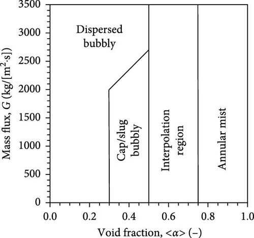
The present study considers upward two-phase flows in vertical pipes. The dispersed two-phase flows are a generic technical term for expressing bubbly, cap bubbly, slug, and churn flows. The separated two-phase flows are used in the present study to express a generic technical term for expressing annular and annular-mist flows. Strictly speaking, annular-mist flows are composed of dispersed liquid droplet flow and separated liquid film flow. Figure 1 shows a typical flow regime map used in the US NRC TRACE code [15]. The flow regime map considers dispersed bubbly and cap/slug bubbly flows as the dispersed two-phase flow regime and annular-mist flows as the separated two-phase flow. The interpolation region expresses the transition region between the separated and dispersed two-phase flows. In the present study, the interpolation region is called the transition two-phase flow regime.
3. Distribution Parameter
3.1. Dispersed Two-Phase Flow Model
3.1.1. Pure Dispersed Two-Phase Flow Regime
The regions with and are referred to as pure dispersed two-phase flow and beyond-dispersed two-phase flow, respectively. The beyond-dispersed flow (DF) includes transition flow between dispersed and annular flow (AF), AF, and annular-mist flow.
3.1.2. Beyond-Dispersed Two-phase Flow Regime
For , local void fraction calculated by Equation (7) at r ≤ xcR is higher than unity and should be reset to unity to use the analytical model with Equations (6), (7), and (10). Figure 2 shows the modification scheme. Here, the nondimensional critical radial position xc is obtained from Equation (7) with α = 1 as:

The nondimensional critical radial position xc is zero at , and Equation (19) is reduced to Equation (15).
3.2. Separated Two-Phase Flow Model
3.2.1. Simple Analytical Model
3.2.2. Ishii’s AF Model
4. Drift Velocity
4.1. Dispersed Two-Phase Flow Model
Analyzing the two-phase flow data collected by Hibiki and Ishii [18] from a 102 mm-diameter pipe, Hibiki and Tsukamoto [16] identified the transition behaviors for drift velocities between bubbly and beyond-bubbly flow regimes as shown in Figure 4. They proposed a correlation for drift velocity applicable to dispersed two-phase flows as:
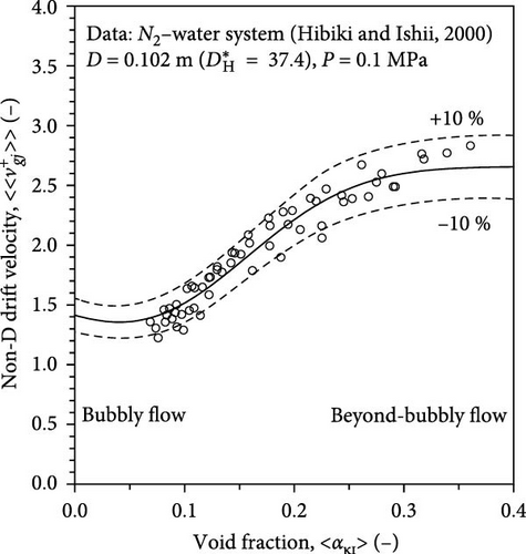
In Equation (51), L is the length scale characterizing a flow channel. For a pipe, a pipe diameter, D, is taken as the characteristic length.
4.2. Separated Two-Phase Flow Model
It should be noted here that Ishii [8] introduced a gravity-correction term in the wall shear stress without its justification, deriving Equation (36). Since it is common not to include such a gravity-correction term in the wall shear stress, the average drift velocity is rederived without the gravity-correction term. The derivation indicates that the constant in the denominator on the right-hand side of Equation (53) becomes 0.010 instead of 0.015 in Equation (36). Here, the rederived average drift velocity gives Equation (53), which is 23% higher than the Ishii’s original average drift velocity. This difference does not cause a significant void fraction prediction difference because the contribution of the drift velocity to a void fraction is negligible in the AF region.
5. Full-Range Drift–Flux Correlation Development
5.1. Distribution Parameter
5.1.1. Critical Void Fraction
It is worth noting that Equation (47) is the advanced version of Equation (61).
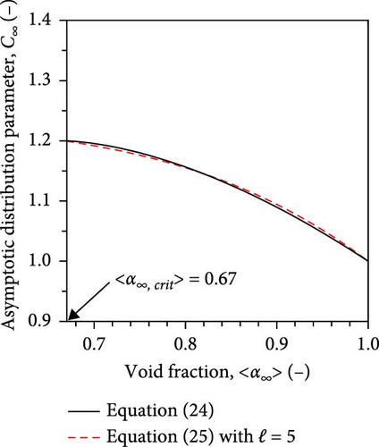
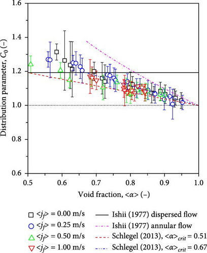
For high void fraction, most flow conditions met , and thus, Equation (60) provides the values of the distribution parameter with reasonable accuracy. Figure 5 presents the variation of the distribution parameters with area-averaged void fractions. Equation (58) slightly underestimates the distribution parameter. However, if the area-averaged void fraction at the transition from cap bubbly to churn-turbulent flows is modified to 0.67, Equation (57) provides excellent prediction accuracy. The modified value corresponds to the critical area-averaged void fraction () obtained by considering a similar distribution of the void fraction and mixture volumetric flux (m∞ = n∞).
5.1.2. Distribution Parameter in Pure Dispersed and Beyond-Dispersed Two-Phase Flows
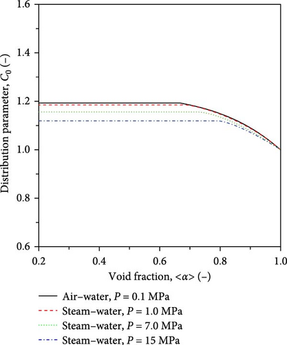
The distribution parameter in pure dispersed and beyond-dispersed two-phase flows is calculated using Equation (9) with Equations (23) and (24) (or (25)). Figure 6 presents the variation of the distribution parameter with area-averaged void fractions. Black solid, red broken, green dotted, and blue chain lines indicate the distribution parameter values for air–water two-phase flows at atmospheric pressure and steam–water two-phase flows at pressures of 1, 7, and 15 MPa, respectively. The critical void fraction between pure dispersed and beyond-dispersed two-phase flows is calculated by Equation (17) with 〈α∞〉 = 0.67. The figure indicates that beyond the critical void fraction, the distribution parameters gradually decrease as the void fraction increases. The distribution parameter for the beyond-dispersed two-phase flow regime tends to approach unity as the void fraction approaches unity.
5.1.3. Distribution Parameter in Separated Two-Phase Flows
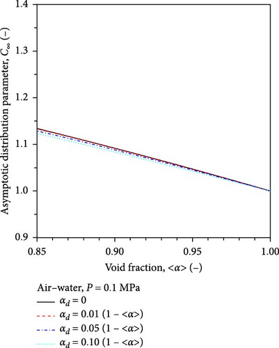
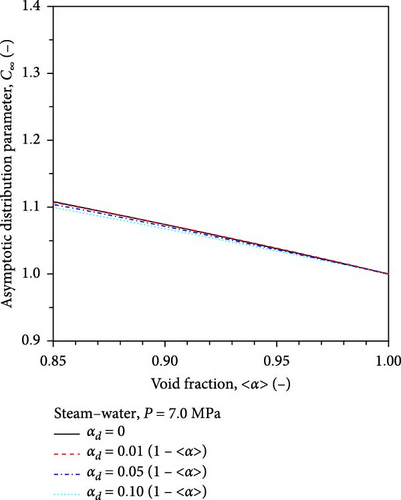
The distribution parameter in separated two-phase flows is calculated by Equations (9) and (33). Figure 7 shows the sensitivity analysis results to examine the effect of assumed entrained liquid droplet fraction on the distribution parameter for separated two-phase flows. Black solid, red broken, green dotted, and blue chain lines indicate the values of the distribution parameters for the steam–water flows at the pressure of 1 MPa, obtained with ξ = 0, 0.01, 0.05, and 0.1, respectively. The figure shows that the entrained liquid droplet fraction has a minor effect on distribution parameters.
5.1.4. Distribution Parameter in Annular Two-Phase Flow
The distribution parameter in AFs is calculated by Equation (37). Figure 8 presents the variation of the distribution parameters in AFs with area-averaged void fraction. Black solid thin, red solid medium-thick and blue solid thick lines indicate the distribution parameter values calculated by Equation (25) for two-phase flow at atmospheric pressure and steam–water two-phase flows at the pressures of 7 and 15 MPa, respectively. Black dotted thin, red dotted medium-thick and blue dotted thick lines indicate the distribution parameter values calculated by Equation (37) for two-phase flows at atmospheric pressure and steam–water two-phase flows at the pressures of 7 and 15 MPa, respectively. Black broken thin, red broken medium-thick and blue broken thick lines are the distribution parameter values calculated by Equation (9) with Equation (35) for two-phase flows at atmospheric pressure and steam–water two-phase flows at the pressures of 7 and 15 MPa, respectively.
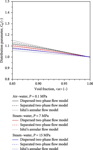
The values of the distribution parameter predicted by Equation (37) are similar to those predicted by Equation (9) with Equation (25) and Equation (9) with Equation (35) for a wide range of density ratios. For 〈α〉 ≥ 0.9, the difference between them is less than 1%. These comparison results suggest that the modeled distribution parameter for beyond-dispersed two-phase flows, Equation (9) with Equation (25), is approximately applicable to separated two-phase flows for the distribution parameter prediction. This significantly simplifies the equation set for a full-range drift–flux correlation.
5.2. Drift Velocity
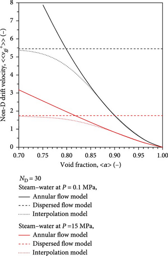
The nondimensional drift velocity in dispersed two-phase flows is calculated using Equation (47). In contrast, the nondimensional drift velocity in annular two-phase flows can be calculated using Equation (54). Figure 9 presents the values of nondimensional drift velocity calculated by Equations (47) and (54). Solid, broken, and dotted lines in Figure 9 represent nondimensional drift velocities predicted using the AF model, Equation (54), DF model, Equation (47), and interpolation model given by:
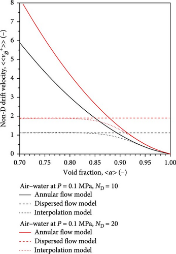
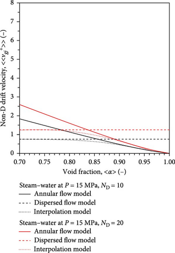
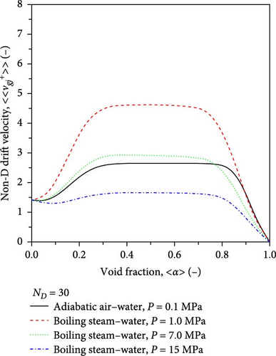
The black thin and red thick lines in Figure 9a show the values of nondimensional drift velocity for ND = 10 and 20, corresponding to 27.3 and 54.6 mm for air–water two-phase flows at atmospheric pressure. The black thin and red thick lines in Figure 9b show the values of nondimensional drift velocity for ND = 10 and 20, corresponding to 10.5 and 21.1 mm for steam–water two-phase flows at the pressure of 15 MPa. The crossover area-averaged void fraction of the two drift velocity models tends to shift toward a low void fraction as the pipe diameter increases. Figure 10 shows the pressure effect on the drift velocity at ND = 30 corresponding to the threshold value between medium and large pipes. The crossover area-averaged void fraction of the two drift velocity models tends to shift toward a low void fraction as the pressure increases. Equation (64) captures the smooth transition of the drift velocity between dispersed and separated two-phase flows.
5.3. Full-Range Drift–Flux Correlation
- •
The critical void fraction is calculated by setting n∞ in Equation (15) at 4, see Equation (65).
- •
C∞ = 1.2 is utilized for the asymptotic distribution parameter of dispersed two-phase flows. Due to the wall-peaking phenomenon in adiabatic bubbly flows and subcooled boiling flows, the distribution parameter in adiabatic bubbly flows and subcooled boiling flows is lower than 1.2. Ishii [8] and Hibiki and Tsukamoto [16] developed the constitutive equations for distribution parameters in adiabatic bubbly flows and subcooled boiling flows given by Equations (66) and (67), respectively.
- •
Equation (25) provides the asymptotic distribution parameter of beyond-dispersed two-phase flows.
The developed full-range drift–flux correlation is summarized as follows:
Distribution parameter
Nondimensional drift velocity
It is worth noting that Equation (72) calculates the nondimensional drift velocity to be zero at 〈α〉 = 1. This results in the term in Equation (70) diverging to infinity at 〈α〉 = 1. When Equation (70) is implemented in a code, special attention should be given at 〈α〉 = 1. In the above equations, the area fraction of liquid entrained in the gas core from the total liquid area is ignored because its effect on void fraction prediction is insignificant. However, the area fraction of liquid entrained in the gas core from the total liquid area should be considered when the liquid fraction 1 − 〈α〉 needs to be calculated accurately.
In the developed full-range drift–flux correlation summarized above, Equations (65) and (68) are analytically developed without any empirical adjustments. Equations (66) and (67) consider the wall-peaking phenomena at low void fraction conditions and have been validated extensively with experimental data. Equation (69) models the flow regime transition from bubbly to beyond-bubbly flows and has been validated with experimental data. The component drift-velocity models for bubbly flows and beyond-bubbly flows in Equation (70) are modeled using a drag law and have been validated with data extensively. Equation (72) derived by Ishii [8] is based on a simple AF model. In contrast to the existing full-range drift–flux correlations, the new full-range drift–flux correlation has been developed based on scientific philosophy to eliminate empiricism as much as possible.
Figure 11 shows the variation of the distribution parameters with the area-averaged void fractions. Solid black, red dotted, broken green, and blue chain lines indicate the values of the distribution parameters for adiabatic air–water two-phase flow at atmospheric pressure and boiling steam–water two-phase flows at pressures of 1.0, 7.0, and 15 MPa, respectively. For adiabatic flows, the distribution parameter is unity at 〈α〉 = 0 and gradually increases to the constant value. Beyond the critical void fraction calculated by Equation (65), the distribution parameter decreases and finally becomes unity at 〈α〉 = 1. For boiling flows, the distribution parameter is zero at 〈α〉 = 0 and sharply increases to the constant value. Beyond the critical void fraction calculated by Equation (65), the distribution parameter decreases and finally becomes unity at 〈α〉 = 1.
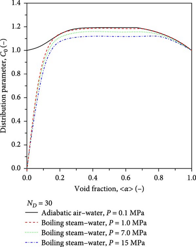
Figure 12 shows the variations of the nondimensional drift velocity with the area-averaged void fractions. Solid black, red dotted, broken green, and blue chain lines indicate the values of the nondimensional drift velocity for adiabatic air–water two-phase flow at atmospheric pressure and boiling steam–water two-phase flows at the pressures of 1.0, 7.0, and 15 MPa, respectively. The nondimensional drift velocity is at 〈α〉 = 0 and gradually decreases due to the increased bubble population. The nondimensional drift velocity increases when large bubbles are formed due to bubble coalescence, and it reaches a constant value. Beyond the crossover area-averaged void fraction, the nondimensional drift velocity starts decreasing and finally becomes zero at 〈α〉 = 1.
6. Results and Discussion
6.1. Existing Database for Upward Two-Phase Flows in Vertical Pipes
The comparison between the experimental and calculated data was made to validate the new full-range drift–flux correlation. In total, 419 experimental data were collected from 9 sources. The specifications of these compiled data are detailed in Table 1. The fluid pairs included air–water, air-kerosene, and air-lube oil. The physical properties of the fluid systems are given in Table 2. The diameters of the test section ranged from 0.6 to 6.7 cm. According to the criteria of the proposed full-range drift–flux correlation, there are 147 experimental data for the pure dispersed two-phase flows and 272 experimental data for the beyond-dispersed flows (DFs). A brief description of each data source is given next.
| Sources | Fluid systems (−) | Diameter, D (cm) | <jf> (m/s) | <jg> (m/s) | Number of data (−) | Measurement methods (−) | Measurement accuracy (%) |
|---|---|---|---|---|---|---|---|
| Beggs [20] | Air–water | 3.84 | 0.0226–2.52 | 0.250–18.1 | 27 | Quick-closing valve | N/A |
| Mukherjee [21] | Air-kerosene and air-lube oil | 3.81 | 0.0274–3.34 | 0.0366–24.3 | 99 | Parallel-plate capacitance | N/A |
| Sujumnong [22] | Air–water | 1.27 | 0.0396–8.46 | 0.0338–59.1 | 83 | Quick-closing valve | N/A |
| Perez [23] | Air–water | 3.8, 6.7 | 0.100–0.730 | 0.126–12.8 | 40 |
|
± 15.0 |
| Kaji and Azzopardi [24] | Air–water | 1.9 | 0.0300–0.650 | 0.865–33.8 | 71 | Conductance probe | ± 10.0 |
| Yan et al. [25] | Air–water | 0.6 | 0.205–1.41 | 0.122–1.94 | 11 | High-speed camera | N/A |
| Wiesche and Kapitz [26] | Air–water | 1.3 | 1.00–2.00 | 1.10–4.63 | 10 | Quick-closing valve | ± 5.7 |
| Bhagwat and Ghajar [27] | Air–water | 1.25 | 0.150–1.05 | 0.170–16.4 | 32 | Quick-closing valve | ± 1.3–± 10.0 |
| Luo et al. [28] | Air–water | 6 | 1.01–1.95 | 20.4–159 | 46 | Quick-closing valve | N/A |
| Fluid systems (−) | σf (mN/m) | ρf (kg/m3) | μf (Pa · s) | ρg(kg/m3) | μg (Pa · s × 106) |
|---|---|---|---|---|---|
| Air–water | 72.0 | 998.0 | 0.000894 | 1.19 | 18.3 |
| Air-kerosene | 22.6–28.8 | 786.6–844.1 | 0.00118–0.00383 | 1.87–7.40 | 16.8–19.6 |
| Air-lube oil | 32.1–37.5 | 832.3–867.7 | 0.0108–0.0744 | 2.23–7.08 | 16.3–19.0 |
6.1.1. The Database of Beggs [20]
Beggs [20] experimentally investigated two-phase flows in inclined pipes. Air and water were used, and a quick-closing valve was adopted to measure the void fractions. Twenty-seven data points obtained for upward two-phase flows in a vertical pipe with a diameter of 3.84 cm were selected here.
6.1.2. The Database of Mukherjee [21]
Mukherjee [21] experimentally investigated upward two-phase flows. Air-kerosene and air-lube oil fluid pairs were used, and a parallel-plate capacitance was adopted to measure the void fractions. One hundred and twelve data points were obtained for a pipe with a diameter of 3.81 cm. However, a data validation process conducted in the present study identified that 13 data points in one experimental run showed physically strange behaviors, indicating the distribution parameter values less than unity in the medium void fraction range. Thus, those data were eliminated in the model validation process.
6.1.3. The Database of Sujumnong [22]
Sujumnong [22] experimentally investigated heat transfer and void fraction for two-phase flows. Air and water were used, and a quick-closing valve was adopted to measure the void fractions. Eighty-three data points obtained for upward two-phase flows in a pipe with a diameter of 1.27 cm were selected here.
6.1.4. The Database of Perez [23]
Perez [23] experimentally investigated two-phase flows in vertical pipes. Air and water were used, and capacitance probes were adopted to measure the void fractions with a measurement accuracy of ± 15.0%. Fifty-three data points obtained for upward two-phase flows in vertical pipes with a diameter of 3.80 or 6.70 cm were selected here. However, a data validation process in the present study identified that 13 data points in one experimental run showed physically strange behaviors, indicating that the distribution parameter values reached 2 in the medium void fraction range. Thus, those data were eliminated in the model validation process.
6.1.5. The Database of Kaji and Azzopardi [24]
Kaji and Azzopardi [24] experimentally investigated two-phase flows in vertical pipes. Conductance probes were used to measure the void fractions with a measurement accuracy of ± 10.0%. Seventy-one data points obtained for upward two-phase flows in a vertical pipe with a diameter of 1.90 cm were selected here.
6.1.6. The Database of Yan et al. [25]
Yan et al. [25] experimentally investigated two-phase flows. Air and water were used, and a high-speed camera was adopted to measure the void fractions. Eleven data points obtained for upward two-phase flows in vertical pipes were selected here.
6.1.7. The Database of Wiesche and Kapitz [26]
Wiesche and Kapitz [26] experimentally investigated two-phase flows in inclined pipes. Air and water were used, and a quick-closing valve was used to measure the void fractions with a measurement accuracy of ± 5.7%. Ten data points obtained for upward two-phase flows in a vertical pipe with a diameter of 1.30 cm were selected.
6.1.8. The Database of Bhagwat and Ghajar [27]
Bhagwat and Ghajar [27] experimentally investigated upward two-phase flows in inclined pipes. Air and water were used, and a quick-closing valve was adopted to measure the void fractions. Thirty-two data points obtained for upward two-phase flows in a vertical pipe with a diameter of 1.25 cm were selected here.
6.1.9. The Database of Luo et al. [28]
Luo et al. [28] experimentally investigated two-phase flows in inclined pipes. Air and water were used, and a quick-closing valve was adopted to measure the void fractions. Forty-six data points obtained for upward two-phase flows in a vertical pipe with a diameter of 6.0 cm were selected here.
6.2. Existing Correlations for Upward Two-Phase Flows in Vertical Pipes
Although research on void fractions for upward two-phase flows has been performed for years, suitable full-range drift–flux correlations are limited. This section briefly reviews the existing full-range drift–flux correlations for upward two-phase flows in vertical pipes.
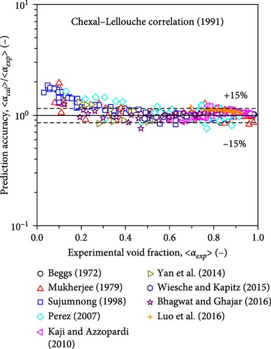
Early in 1991, Chexal et al. [11] proposed a full-range drift–flux correlation, the Chexal–Lellouche correlation (1991) or EPRI correlation, for void fraction prediction of two-phase flows. The applicable range of orientations was from − 90° to + 90°, where − 90° represented downward flows in vertical pipes and + 90° represented upward flows in vertical pipes. The Chexal–Lellouche correlation (1991) covered the full range of void fractions from 0 to 1. The Chexal–Lellouche correlation (1991) was established based on a large amount of experimental data, and many cascading constitutive equations and empirical parameters were used. One of the modeling deficiencies for the Chexal–Lellouche correlation (1991) is that the value of the distribution parameter for adiabatic flows approaches zero as the void fraction approaches zero. Hibiki and Ishii [18] experimentally demonstrated that the value of the distribution parameter for adiabatic flows was around unity at small void fractions. The prediction accuracy of the Chexal–Lellouche correlation (1991) is expected to deteriorate at low void fraction conditions.
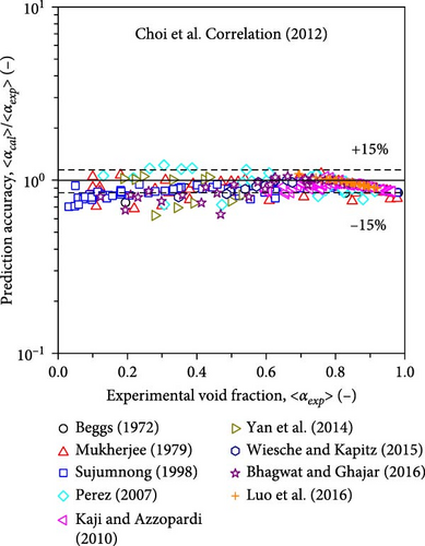
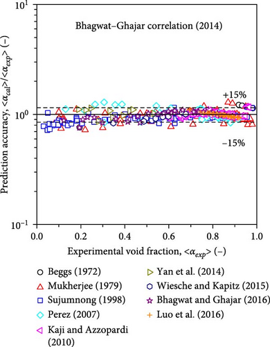
Choi et al. [12] developed a drift–flux correlation, the Choi et al. correlation (2012), by combining the Fabre and Line correlation (1992) [13] and the Ishii correlation (1977) [8]. Bhagwat and Ghajar [14] also proposed a full-range drift–flux correlation, the Bhagwat–Ghajar correlation (2014), based on experimental data. Similar to the Chexal–Lellouche correlation (1991) and the Choi et al. correlation (2012), the Bhagwat–Ghajar correlation (2014) was also expressed in implicit form, and iteration was necessary to calculate the void fractions. One of the modeling deficiencies for the Choi et al. correlation (2012) and the Bhagwat–Ghajar correlation (2014) is that the value of the distribution parameter approaches 2 as the two-phase Reynolds number approaches zero. A minimal two-phase Reynolds number condition corresponds to a condition with a minimal superficial gas velocity for a pool system. A simple thought experiment indicates that such a flow condition cannot produce steep void fraction and mixture volumetric flux distributions at a pipe center. Thus, the value of the distribution parameter should be of the order of unity. The prediction accuracy of the Choi et al. correlation [12] and the Bhagwat–Ghajar correlation (2014) is expected to deteriorate at low two-phase Reynolds number conditions.
The detailed expressions of the Chexal–Lellouche correlation (1991), the Choi et al. correlation (2012), and the Bhagwat–Ghajar correlation (2014) are given in Table 3.
| Researcher | Drift–flux correlation |
|---|---|
| Chexal–Lellouche correlation (1991) |
|
| Choi et al. correlation (2012) |
|
| Bhagwat–Ghajar correlation (2014) |
|
6.3. Assessment of Existing Full-Range Drift–Flux Correlations With Existing Data
Here N, 〈α〉cal, and 〈α〉exp represent the number of data, the calculated void fractions, and the experimental void fractions.
Figure 13 compares the measured void fractions and those calculated using the Chexal–Lellouche correlation (1991), the Choi et al. correlation (2012), and the Bhagwat–Ghajar correlation (2014). The database that was compiled as described in Section 6.1 was used. Since the Chexal–Lellouche correlation (1991), the Choi et al. correlation (2012), and the Bhagwat–Ghajar correlation (2014) were claimed as full-range correlations applicable to 0 ≤ 〈α〉 ≤ 1.0, the experimental data used in the present study fell within the applicable ranges of the existing correlations. These three correlations could reasonably predict the data at higher void fractions. However, as explained in Section 6.2, the deviations between the measured and calculated values increased at lower void fractions. Table 4 presents the statistical parameters of these drift–flux correlations, and mrel, ab, ranged from 7.78% to 10.8%. It should be noted that all these existing drift–flux correlations were developed based on complicated and cascaded functional forms. Thus, if these correlations are applied to flow conditions beyond the validated conditions, special cautions are necessary.
| Model | md (−) | sd (−) | mrel (%) | mrel, ab (%) |
|---|---|---|---|---|
| Chexal–Lellouche correlation (1991) | 0.0264 | 0.0596 | 4.87 | 9.36 |
| Choi et al. correlation (2012) | − 0.0489 | 0.0514 | − 9.70 | 10.8 |
| Bhagwat–Ghajar correlation (2014) | − 0.00237 | 0.0634 | − 2.63 | 7.78 |
6.4. Evaluation of Developed Full-Range Drift–Flux Correlation Using Existing Data
6.4.1. Validation Using the Database of Sujumnong [22]
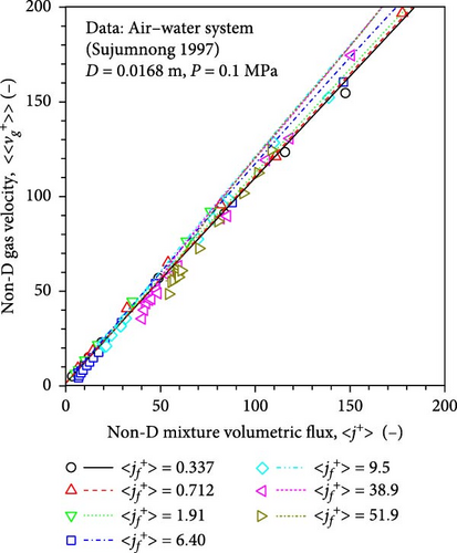
Figure 14a presents the drift–flux plot for air–water flows in a round pipe (diameter, 12.7 mm) taken from Sujumnong [22]. Each data group was plotted by changing the superficial gas velocity at a fixed superficial liquid velocity. The increase in the mixture volumetric flux corresponded to the increase in the superficial gas velocity. The black circles, red triangles, green inverted triangles, blue squares, cyan diamonds, pink left-pointing triangles, and dark yellow right-pointing triangles represent the data taken at , , , , , , and , respectively. The black solid, red dashed, green dotted, blue chain, cyan double chain, pink short dashed, and dark yellow short chain lines represent the calculated nondimensional gas velocities obtained using the newly-developed full-range drift–flux correlation at fixed superficial liquid velocities. It was observed that the calculated nondimensional gas velocities agreed well with the experimental data.
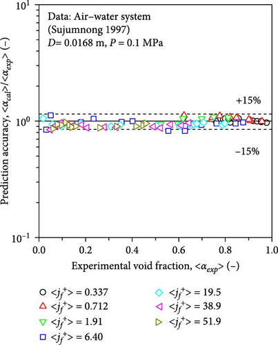
Although the data were not adopted in developing the full-range drift–flux correlation, excellent agreement was observed between the experimental and calculated void fractions, as shown in Figure 14b, validating the modeling concept used in the present study. Among the calculated void fractions, 96.2% of them were within the ± 15% error band. The md, sd, mrel, and mrel, ab were − 0.00855, 0.0371, − 4.12%, and 7.14%, respectively.
6.4.2. Validation Using the Database of Kaji and Azzopardi [24]
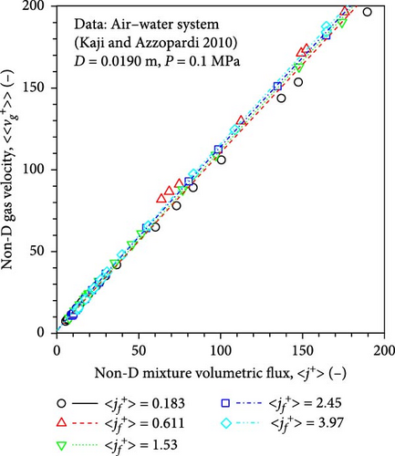
Figure 15a presents the drift–flux plot for air–water flows in a round pipe (diameter, 19.0 mm). The experimental data were taken from Kaji and Azzopardi [24]. The black circles, red triangles, green inverted triangles, blue squares, and cyan diamonds represent the data taken at , , , , and , respectively. The black solid, red dashed, green dotted, blue chain, and cyan double chain lines represent the calculated nondimensional gas velocities by the newly developed full-range drift–flux correlation at fixed superficial liquid velocities. It was observed that the calculated nondimensional gas velocities agreed well with the experimental values.
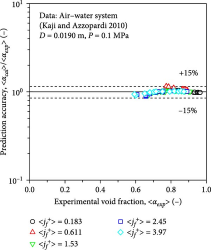
Although the data were not adopted in developing the full-range drift–flux correlation, excellent agreement was observed between the experimental and calculated void fractions, as shown in Figure 15b, validating the modeling concept used in the present study. Among the calculated void fractions, 97.2% of them were within the ± 15% error band. The md, sd, mrel, and mrel, ab were 0.00932, 0.0347, 0.739%, and 3.34%, respectively.
6.4.3. Validation Using the Database of Wiesche and Kapitz [26]
Figure 16a presents the drift–flux plot for air–water flows in a round pipe (diameter, 13.0 mm). The experimental data were taken from Wiesche and Kapitz [26]. The black circles and red triangles represent the data taken at and , respectively. The black solid and red dashed lines represent the calculated nondimensional gas velocities by the newly developed full-range drift–flux correlation at fixed superficial liquid velocities. It was observed that the calculated nondimensional gas velocities agreed well.
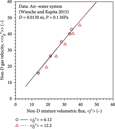
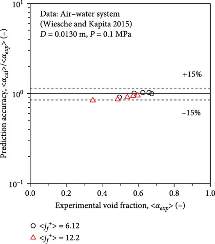
Although the data were not adopted in developing the full-range drift–flux correlation, excellent agreement was observed between the experimental and calculated void fractions, as shown in Figure 16b, validating the modeling concept used in the present study. Almost all of the calculated void fractions were within the ± 15% error band. The md, sd, mrel, and mrel, ab were − 0.0228, 0.0315, − 5.79%, and 7.17%, respectively.
6.4.4. Validation Using the Database of Bhagwat and Ghajar [27]
Figure 17a presents the drift–flux plot for air–water flows in a round pipe (diameter, 12.5 mm). The experimental data were taken from Bhagwat and Ghajar [27]. The black circles, red triangles, green inverted triangles, and blue squares represent the data taken at , , , and , respectively. The black solid, red dashed, green dotted, and blue chain lines represent the calculated nondimensional gas velocities by the newly developed full-range drift–flux correlation at fixed superficial liquid velocities. It was observed that the calculated nondimensional gas velocities agreed well with the experimental data.
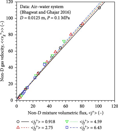
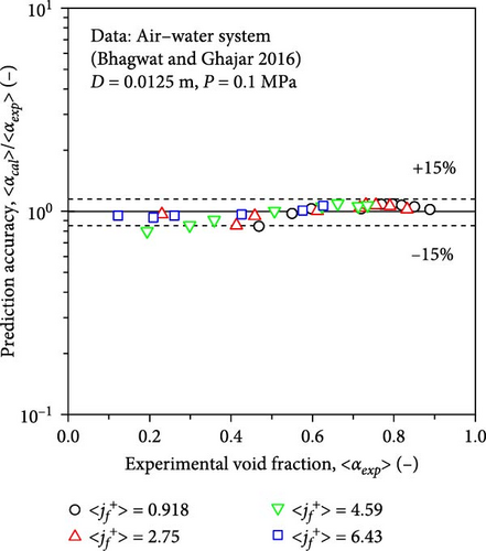
Although the experimental data were not considered in the model development, excellent agreement was observed between the experimental and calculated void fractions, as shown in Figure 17b. Among the calculated void fractions, 96.7% of them were within the ± 15% error band without systematic deviations. The md, sd, mrel, and mrel, ab were 0.0139, 0.0391, − 0.571%, and 6.76%, respectively.
6.4.5. Validation of the Newly Developed Full-Range Drift–Flux Correlation Using the Compiled Database and Boiling Flow Data
Figure 18 compares the measured void fractions and those calculated using the compiled database (Tables 1 and 2). Excellent agreement was seen over the full range of void fractions 〈α〉 from 0 to 1.0. More than 90% of the calculated values were within the ± 15% error band without any systematic deviations. Table 5 summarizes the statistical parameters for each dataset when the developed correlation was employed. To evaluate the proposed full-range drift–flux correlation for each flow regime, the performance indices of the proposed correlation for pure dispersed two-phase flow and beyond-dispersed two-phase flow were obtained. The md, sd, mrel, and mrel, ab in the pure dispersed two-phase flow regime were − 0.0110, 0.0370, − 3.65%, and 8.41%, respectively. The md, sd, mrel, and mrel, ab in the beyond-dispersed two-phase flow regime, including transition flow between dispersed and AF, AF, and annular-mist flow, were 0.00948, 0.0513, 0.915%, and 4.98%, respectively. The overall md, sd, mrel, and mrel, ab in the full void fraction range were 0.00230, 0.0480, − 0.686%, and 6.18%, respectively. It should be noted here that the mrel, ab ( = 6.18%) does not include the measurement uncertainty. If measurement uncertainty of 10% or 15% is considered, the mean absolute relative deviation becomes 11.8% and 16.2%, respectively.
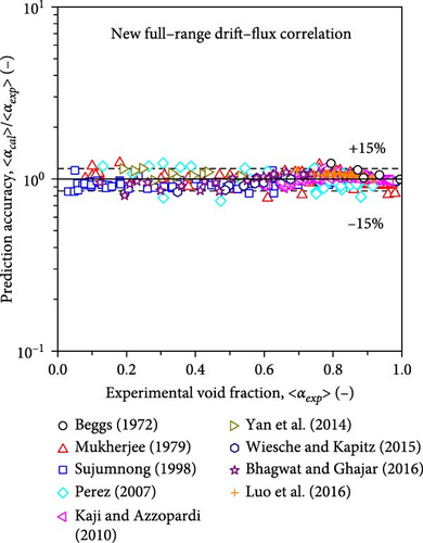
| Data source | md (−) | sd (−) | mrel (%) | mrel, ab (%) |
|---|---|---|---|---|
| Beggs [20] | − 0.0268 | 0.0168 | − 4.67 | 4.98 |
| Mukherjee [21] | 0.0181 | 0.0617 | 3.37 | 8.21 |
| Sujumnong [22] | − 0.00855 | 0.0371 | − 4.12 | 7.14 |
| Perez [23] | − 0.0254 | 0.0231 | − 3.95 | 10.6 |
| Kaji and Azzopardi [24] | 0.00932 | 0.0347 | 0.739 | 3.34 |
| Yan et al. [25] | 0.0213 | 0.0464 | 6.21 | 6.56 |
| Wiesche and Kapitz [26] | − 0.0228 | 0.0315 | − 5.79 | 7.17 |
| Bhagwat and Ghajar [27] | 0.0139 | 0.0391 | − 0.571 | 6.76 |
| Luo et al. [28] | 0.0393 | 0.0200 | 4.52 | 4.52 |
| Total | 0.00230 | 0.0480 | − 0.686 | 6.18 |
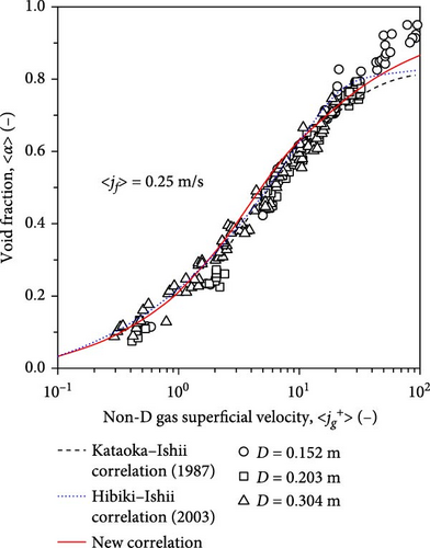
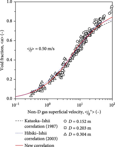
To further evaluate the prediction performance of the full-range drift–flux correlation, the comparison between the newly developed model and other flow regime-based drift–flux models was performed, as shown in Figure 19. The dataset used in Figure 19 was selected from Schlegel et al. [19] with fixed superficial liquid velocities of 0.25, 0.50, and 1.0 m/s. The black dashed, blue dotted, and red solid lines represent the calculated values obtained by the Kataoka–Ishii correlation (1987), the Hibiki–Ishii correlation (2003), and the newly developed full-range drift–flux correlation. The Kataoka–Ishii correlation (1987) was developed for cap-bubbly and churn-turbulent flow regimes in pool conditions, while the Hibiki–Ishii correlation (2003) was developed for bubbly and cap-bubbly flows in large-diameter pipes. The newly developed full-range drift–flux correlation could calculate the void fractions of all the flow regimes, including dispersed and separated two-phase flows, accurately. The excellent prediction performance of the newly developed full-range drift–flux correlation was due to the accurately modeled distribution parameter and drift velocity, which approached unity and zero as the void fraction approached unity.

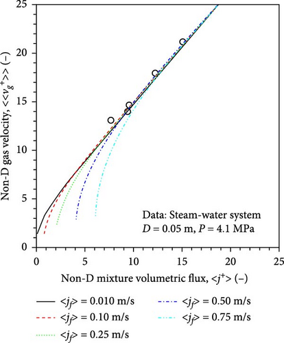
The application of the proposed full-range drift–flux correlation to the steam–water database is discussed. The steam–water data were taken from Petrick [29]. The diameter and pressure in Petrick [29] were 0.05 m and 4.1 MPa, respectively. Since only the steam velocity and mixture volumetric flux data were available, the present study plotted the calculated steam velocities with the mixture volumetric flux at fixed superficial liquid velocities. Figure 20 presents the drift–flux plot using the steam–water database collected from Petrick [29] at p = 4.1MPa. The black solid, red dashed, green dotted, blue chain, and cyan double chain lines represent the calculated nondimensional gas velocities by the newly developed full-range drift–flux correlation at fixed superficial liquid velocities of 〈jf〉 = 0.010, 0.10, 0.25, 0.50, and 0.75 m/s, respectively. A consistent trend of the nondimensional gas velocities with the nondimensional mixture volumetric flux is observed, suggesting the applicability of the proposed full-range drift–flux correlation to steam–water flows.
7. Conclusions
- •
The critical area-averaged void fraction 〈α〉crit at the onset of the transition from pure dispersed to beyond-dispersed two-phase flows was estimated by Equation (17) with = 0.67 by considering that the similar distributions of the void fraction and mixture volumetric flux at negligibly small Nρ were similar (m∞ = n∞).
- •
The constitutive equations of distribution parameter and drift velocity for upward cocurrent two-phase flows, including pure dispersed and beyond-dispersed two-phase flow regimes and separated two-phase flows, were analytically derived.
- •
An extensive literature review on void fractions for upward two-phase flows in vertical pipes was made, and 419 experimental data were collected from nine sources. The existing full-range drift–flux correlations were also reviewed. The performance evaluation of the existing correlations using the compiled database indicated that none of the existing correlations could predict the whole range of void fraction data with acceptable accuracy.
The developed full-range drift–flux correlation was validated using the compiled database with the following statistical indices being obtained: mean relative deviation, mrel, − 0.686%; and mean absolute relative deviation, mrel, ab, 6.18%. The validated range of the proposed correlation is: 0.6 cm ≤ D ≤ 6.7 cm, 0.0338 m/s ≤ 〈jg〉 ≤ 159m/s, and 0.0226 m/s ≤ 〈jf〉 ≤ 8.46m/s.
Nomenclature
-
- C0:
-
- Distribution parameter (−)
-
- C∞:
-
- Asymptotic distribution parameter (−)
-
- D:
-
- Pipe diameter (m)
-
- Ed:
-
- Area fraction of liquid entrained in the gas core (−)
-
- g:
-
- Gravitational acceleration (m/s2)
-
- j:
-
- Mixture volumetric flux (m/s)
-
- jf:
-
- Superficial liquid velocity (m/s)
-
- jg:
-
- Superficial gas velocity (m/s)
-
- j0:
-
- Mixture volumetric flux at the pipe center (m/s)
-
- :
-
- Exponent: (−)
-
- L:
-
- Length (m/s)
-
- La:
-
- Laplace length (m)
-
- m:
-
- Exponent to control the distribution of the mixture volumetric flux (−)
-
- ND:
-
- Nondimensional hydraulic equivalent diameter defined by L/La (−)
-
- Nμf:
-
- Viscosity number for liquid phase (−)
-
- Nρ:
-
- Density ratio (−)
-
- n:
-
- Exponent to control the distribution of the void fraction (−)
-
- R:
-
- Pipe radius (m)
-
- r:
-
- Radial distance measured from the pipe center (m)
-
- :
-
- Average drift velocity (m/s)
-
- vg:
-
- Gas velocity (m/s)
-
- vgj:
-
- Drift velocity (m/s)
-
- vr:
-
- Relative velocity between gas and liquid phases (m/s)
-
- x:
-
- Nondimensional radial position (−)
-
- xB:
-
- Nondimensional radial location of the gas–liquid interface (−)
Greek Symbols
-
- α:
-
- Void fraction (−)
-
- α0:
-
- Void fraction at the pipe center (−)
-
- αd:
-
- Entrained liquid droplet fraction (−)
-
- αw:
-
- Void fraction at the pipe wall (−)
-
- Δρ:
-
- Density difference (kg/m3)
-
- θ:
-
- Inclination angle (°)
-
- μ:
-
- Dynamic viscosity (Pa · s)
-
- ρf:
-
- Density of liquid (kg/m3)
-
- ρg:
-
- Density of gas (kg/m3)
-
- σ:
-
- Surface tension (N/m)
Subscripts
-
- AF:
-
- Annular flow (−)
-
- Cal:
-
- Calculated (−)
-
- critical:
-
- Critical value (−)
-
- DF:
-
- Dispersed flow (−)
-
- Exp:
-
- Experimental (−)
-
- Ishii:
-
- Value calculated by Ishii model (1977) (−)
-
- KI:
-
- Value calculated by Kataoka–Ishii model (1987) (−)
-
- ∞:
-
- Asymptotic value or negligibly small Nρ (−)
Superscripts
-
- +:
-
- Nondimensional value (−)
Mathematical Symbols
-
- 〈 〉:
-
- Area-averaged quantities (−)
-
- 〈〈 〉〉:
-
- Void fraction-weighted quantities (−).
Disclosure
This work was performed under the auspices of the Secretariat of the Nuclear Regulation Authority of Japan.
Conflicts of Interest
The authors declare no conflicts of interest.
Author Contributions
Takashi Hibiki: conceptualization, formal analysis, methodology, writing, supervision, project administration, data curation, validation, funding acquisition. Chuanshuai Dong: writing – original draft, methodology, investigation, formal analysis, validation. Naofumi Tsukamoto: conceptualization, writing – review and editing.
Funding
This research was supported by the Secretariat of the Nuclear Regulation Authority of Japan Hong Kong SAR Government Hong Kong Jockey Club.
Acknowledgments
One of the authors (Takashi Hibiki) would like to express his sincere appreciation to the Secretariat, to the Hong Kong SAR Government for supporting his research under the Global STEM Professorship, and to the Hong Kong Jockey Club for supporting his research under the JC STEM Lab of Innovative Thermo-Fluid Science.
Open Research
Data Availability Statement
The data that support the findings of this study are available from the corresponding author upon reasonable request.


