Assessment of Different Turbulence Models on Melt Pool Natural Convection Simulations With Internal Heat Source
Abstract
In the context of severe nuclear accidents, the migration of corium into the reactor pressure vessel (RPV) poses significant hazards, prompting the proposal of the in-vessel melt retention (IVR) strategy, particularly the external reactor vessel cooling (ERVC) approach. Evaluating the accuracy of turbulence models within the melt pool is crucial for assessing the feasibility of IVR. However, previous studies have yet to reach a consensus about the most suitable model due to the lack of data comparison. We aim to conduct a comprehensive comparative analysis of turbulence models to evaluate their performance across a range of Rayleigh numbers, particularly under conditions relevant to IVR scenarios. Therefore, this study employs six commonly used turbulence models in computational fluid dynamics (CFD) software, ANSYS Fluent, to simulate three natural convection experiments (Kulacki–Goldstein, BALI, and LIVE-3D). The results demonstrate that the choice of turbulence model significantly impacts the accuracy of temperature and heat flux predictions within the melt pool. Although the relative temperature deviation is less than 0.1% in all the simulations of the Kulacki–Goldstein experiment, the differences among turbulence models become increasingly pronounced with rising Rayleigh numbers. Among the models tested, wall-modeled large eddy simulation (WMLES) proved the most reliable for complex geometries and high Rayleigh numbers, while the realizable k-epsilon and generalized k-omega (GEKO) models also showed consistent performance. However, the Reynolds stress model (RSM)–baseline (BSL) and detached eddy simulation (DES) models exhibited notable limitations, particularly in scenarios involving solidification and melting. These findings provide valuable guidance for selecting appropriate turbulence models in IVR-related natural convection simulations and highlight the need for further refinement to improve model accuracy across varying melt pool conditions.
1. Introduction
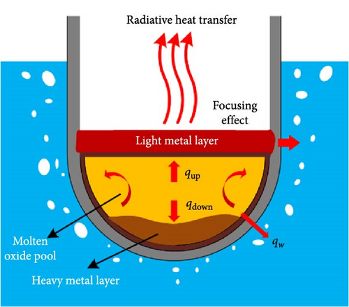
In the event of a severe nuclear accident, the migration and relocation of the corium into the lower head of the reactor pressure vessel (RPV) pose a significant risk, potentially leading to breaches and the release of radioactive materials into containment [1]. To mitigate this risk, the in-vessel melt retention (IVR) strategy, particularly the external reactor vessel cooling (ERVC) approach, has been proposed [2–4]. By injecting water into the cavity and utilizing heat transfer mechanisms, this method aims to contain the melt within the RPV, safeguarding its structural integrity, and preventing the release of the melt [5], as shown in Figure 1.
Numerical simulations have emerged as a promising alternative for predicting heat flux and temperature distribution within the RPV’s lower head. Two primary numerical methods, lumped parameter models [2, 13–18], and computational fluid dynamics (CFD) models [19–28], have been employed for this purpose. Among these, CFD models have gained popularity due to their versatility and ability to provide detailed insights into internal flow characteristics. However, accurately simulating natural convection in high Ra′ melt pools, characterized by large-scale turbulent flow and intense turbulence mixing, remains a challenge.
The choice of turbulence model significantly impacts the accuracy of simulation outcomes in CFD models. In CFD, turbulence can be treated in various ways: fully resolved with direct numerical simulation (DNS), partially resolved with large eddy simulation (LES), fully modeled with reynolds-averaged Navier–Stokes (RANS), or using hybrid LES/RANS schemes like detached eddy simulation (DES). Within RANS, there are different submodels, such as the k-omega model, the k-epsilon model, and the Reynolds stress model (RSM). Various turbulence models have been used in previous studies [24–29]. Dinh and Nourgaliev [24] analyzed natural convection in a melt pool of water with internal heat sources at high Ra′ numbers (up to 1015) using the modified low-Reynolds number (LRN) model. Fukasawa, Hayakawa, and Saito [25] simulated the BALI experiment using LES and the LRN models in PHOENICS software. Zhang et al. [27] numerically simulated and validated the BALI, LIVE, and COPRA experiments using the algebraic wall-modeled LES (WMLES) model in ANSYS Fluent software. Aounallah et al. [26] utilized RANS models and coarse grid DNS models for natural convection in a heated cavity (Ra′ = 109−1012, Pr = 0.71). Bian, Villanueva, and Dovizio [28] conducted the DNS simulation of internally heated natural convection in a 3D semicircular molten pool using Nek5000 (Ra′ = 1011, Pr = 3.11). Wei and Chen [29] investigated the influence of different turbulence models on the transient temperature and velocity distribution of the COPRA water experiment using ANSYS Fluent. The RNG k-epsilon and realizable k-epsilon turbulence models, incorporating full buoyancy effects, along with the DES (Spalart–Allmaras) and DES (shear–stress transport [SST] k-omega) turbulence models, are recommended for accurately capturing large-scale natural convection behavior [29]. Shams [30] compared the linear low-Reynolds k-epsilon model, the nonlinear Reynolds stress model (RSM-EB), and the algebraic heat flux model (AHFM-NRG) in the STAR-CCM + simulation of BALI experiments. They found that all of the previous models struggled to capture complex heat transfer phenomena. Hence, an AHFM-NRG + model is proposed through calibration of the AHFM-NRG model [30]. Sharma et al. [31] accurately predicted natural convection in the BALI experiment, pressurized water reactor (PWR) and boiling water reactor (BWR) geometries using the algebraic heat flux models (AHFM Default, AHFM-2005). However, comparative data on their performance in simulating natural convection within melt pools are limited, and there is currently no consensus on the most suitable model.
We have chosen three candidate experiments: the Kulacki–Goldstein [32], LIVE-3D [33], and BALI [9] experiments, which represent three distinct shape categories: 2D rectangular slice, 3D hemisphere, and 2D quarter-circle slice. It is worth noting that the internal Rayleigh numbers in the BALI experiments reach levels comparable to those in prototype conditions. Although the Kulacki–Goldstein experiment is conducted at a relatively low Rayleigh number, the electrode-heating method employed ensures uniform heating, and it is one of the few experiments that provides DNS data. The LIVE-3D experiment, with its 3D hemispherical melt pool, realistically simulates the shape of the melt pool in the lower head of an actual reactor, and it also incorporates a more accurate representation of the core conditions through the simulation of solidifying and melting materials. Table 1 provides a detailed comparison of the experimental setup, including information on their geometric diversity, simulants, Rayleigh number ranges, and other parameters.
| Experimental characteristics | Kulacki–Goldstein | LIVE-3D | BALI |
|---|---|---|---|
| Geometry shape | 2D-rectangle | 3D-hemisphere | 2D-quarter circular slice |
| Dimensions |
|
R = 0.5 m | R = 2 m, d = 0.15 m |
| Working fluid | AgNO3 solution (Pr = 6–7) | 20%NaNO3-80%KNO3 (Pr = 6.35–10.36) | Salt water (Pr ≈ 7) |
| Heating method | Electrode heating | Planar resistance wire heating | Electrode grids heating |
| Boundary conditions | Top and bottom walls cooling, sidewalls adiabatic | Top cooling/adiabatic, curved bottom wall cooling | Top cooling/adiabatic, curved walls cooling, and vertical walls adiabatic |
| Ra’ | 106 | 1013 | 1015−1017 |
This paper aims to address this gap by comparing six commonly used turbulence models through the simulation of three natural convection experiments. By providing insights into the selection and accuracy of different turbulence models including RANS, DES, and LES, this study seeks to contribute to the development of more reliable predictive capabilities for IVR strategies. In this paper, after introducing the turbulence models in Section 2, we present the simulation and comparison results with experimental data in Sections 3–5. Finally, the selection of current turbulence models is discussed in Section 6.
2. Numerical Model and Simulation Setup
2.1. Governing Equations and Turbulence Model Assumptions
The source Sm is the mass added to the continuous phase from the dispersed second phase and any user-defined sources.
Currently, it is almost impossible to apply the DNS method for turbulence simulation in the industry aspect, therefore other turbulence models need to be used for the simulation of turbulence behavior [34].
- 1.
SST k-omega model.
- 2.
Generalized k-omega (GEKO) model.
- 3.
Realizable k-epsilon model (enhanced wall treatment).
- 4.
Reynolds stress model (RSM-BSL).
- 5.
Detached eddy simulation (DES-k-omega).
- 6.
WMLES model.
- 1.
The SST k-omega model combines the k-epsilon and k-omega models such that the k-omega is used in the inner region of the boundary layer and switches to the k-epsilon in the free shear flow. These features make the SST k-omega model more accurate and reliable for a wider class of flows [35].
- 2.
The GEKO model, developed by ANSYS, is a modification of the standard k-omega model, equipped with four flexible parameters and robust default values. Rather than necessitating different models for various flow scenarios, the adjustable parameters of the GEKO model offer a unified solution to a wide range of applications [36, 37].
- 3.
The realizable k-epsilon model improves upon the standard k-epsilon model by using a different formulation for turbulent viscosity and a modified equation for dissipation rate. Enhanced wall treatment for the k-epsilon equation is a near-wall modeling method that combines a two-layer model with enhanced wall functions. If the near-wall mesh is fine enough to be able to resolve the viscous sublayer.
- 4.
The RSM is the most elaborate RANS turbulence model offered by ANSYS Fluent. Unlike simpler models, RSM abandons the isotropic eddy-viscosity assumption and closes the RANS equations by solving transport equations for Reynolds stresses and the dissipation rate. This requires solving five additional equations in 2D and seven in 3D.
-
The above four models are categorized as the RANS models which consider Reynolds stresses by solving transport equations and dissipation rates. The LES model is a turbulence simulation approach that resolves large-scale turbulent structures while modeling the effects of smaller scales, providing high accuracy in capturing complex flow dynamics. DES and WMLES Models are hybrid LES/RANS models. The computational cost is lower than LES but higher than RANS. DES focuses more on separating flows, while WMLES focuses on simplified boundary layer processing through wall models to deal more effectively with high Reynolds number turbulence.
- 5.
In the DES method, the near-wall region is simulated by the unsteady RANS (URANS) turbulence models, and the other separated regions are simulated by the LES method.
- 6.
To enhance consideration of near-wall gradient effects, an algebraic WMLES model was proposed by Shur et al. [38], which is a combination of a mixing length model with a modified Smagorinsky subgrid-scale (SGS) turbulence model [39], incorporating Piomelli’s wall-damping function [39]. In WMLES, eddy viscosity is calculated by using the mixing length scale.
Buoyancy effects are activated in both the k and ε/ω equations during the calculations. The first cell height for these turbulence models meets the requirement of y+ < 1. The detailed equations for each turbulence model can be found in the Appendix.
2.2. Numerical Methods
To simulate 3D natural convection in ANSYS Fluent, start by creating the geometric model using ANSYS SpaceClaim. Next, generate a suitable mesh in ANSYS Meshing or ICEM, ensuring that the grid is sufficiently refined in the flow region, particularly near the boundary layers. In ANSYS Fluent, select double precision and choose the pressure-based solver, enabling gravity and setting its direction. Turn on the energy equation to couple the flow and heat transfer in natural convection. Input the physical properties of the fluid, such as density, viscosity, and thermal conductivity. Specifying the reference density and volumetric expansion coefficient allows the Boussinesq model to appropriately handle density changes due to temperature, effectively simulating natural convection phenomena.
Next, set the uniform volumetric heat source in the cell zone properties, specifying the heat generation rate per unit volume. Define suitable boundary conditions for the walls, which may include adiabatic or constant temperature conditions. Use “Body Force Weighted” or “PRESTO!” for the discretization of the momentum equation. Use transient solving to allow the flow and thermal fields to evolve over time, monitoring key parameters to identify when steady-state conditions are achieved.
Once the simulation is complete, utilize CFD-post to analyze the results, visualizing velocity and temperature distributions, heat flux, and other flow characteristics.
3. Experiment 1: Kulacki–Goldstein Experimental Simulation
3.1. Experimental Overview
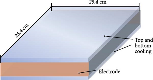
Kulacki–Goldstein experiment studied natural convection heat transfer in a horizontal rectangular fluid layer with a uniform volumetric heat source, as depicted in Figure 2. The fluid is contained in a tank with a base area of 0.254 m × 0.254 m, and the case of H = 3.176 cm is chosen in this research, which corresponds to Ra′ = 106. The working fluid used in the experiment is an AgNO3 aqueous solution with a Prandtl number of approximately 6–7, and the uniform volumetric heat source is achieved through electrode heating. The upper and lower walls are kept at a constant temperature through water cooling, while the surrounding walls have adiabatic boundary conditions [32].
3.2. Simulation Setup
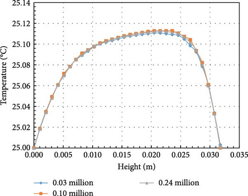
The fluid properties and boundary conditions in the simulation are set according to the experiment. The hexahedral mesh for the computational domain is generated using the ANSYS ICEM meshing tool. The initial temperature of the liquid is 25°C, with a volumetric heat source of 926.7 W/m³. Other parameters are listed in Table 2. The density of water is set using the Boussinesq model. The top and bottom walls are maintained at a constant temperature of TW = 25°C, while all other sides are adiabatic, as illustrated in Figure 3. For the mesh independence test, the k-omega SST turbulence model is used, and the first layer thickness is adjusted to ensure a nondimensional wall distance (y+ < 1). Figure 4 shows that a mesh with 0.10 million elements provides mesh-independent results and is selected for subsequent calculations.

| Symbol | Parameter name | Unit | Value |
|---|---|---|---|
| ρ | Reference density | kg/m3 | 997.15 |
| Cp | Specific heat capacity | J/kg·K | 4176.8 |
| λ | Thermal conductivity | W/m·K | 0.605 |
| μ | Viscosity | kg/m·s | 8.99E−04 |
| β | Thermal expansion coefficient | 1/K | 2.58E−04 |
3.3. Simulation Results
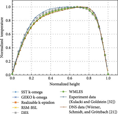
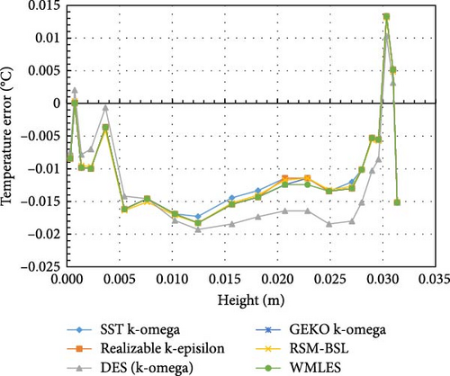
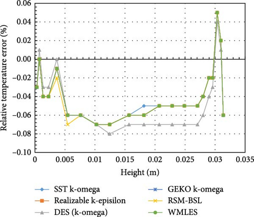
Various turbulence models introduced at the beginning of Section 2 are used to simulate the Kulacki–Goldstein experiment. As Figure 5, the absolute temperature range from the simulation aligns well with the data from the Kulacki–Goldstein experiment, considering the experimental error. After correcting for systematic errors in the wall temperature gradients due to refraction, the total experimental uncertainty in the computed Nusselt number ranged from ±3.2% to ±6.5% [32]. Figure 6 illustrates the normalized temperature values from the calculated turbulence models compared to DNS results and experimental data. It can be seen that the relative temperature values calculated from various turbulence models lie between the DNS and experimental results, indicating that all these models are reliable.

3.4. Comparison With Experimental Data
To further evaluate the computational accuracy of each turbulence model, the absolute and relative errors between the simulated temperature and the experimental data at corresponding heights are shown in Figures 7 and 8. It is observed that all turbulence models showed relatively small deviations (<0.1%) at this scale.
4. Experiment 2: LIVE-3D Experimental Simulation
4.1. Experimental Overview
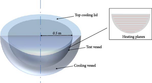
One of the most well-known experiments conducted in a hemispherical pool is the LIVE-3D experiment. As shown in Figure 9, the LIVE-3D experimental apparatus is a 1 : 5 scale replica of the lower plenum of a PWR. The test facility has a diameter of 1 m, and the Rayleigh number (Ra′) in this experiment is approximately 1013. A noneutectic binary mixture of 20% NaNO3 and 80% KNO3 (molar fraction) is used as the simulant material [40].
4.2. Simulation Setup
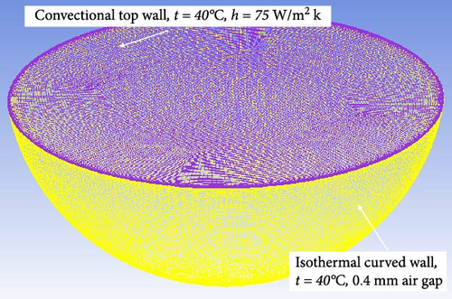
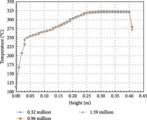
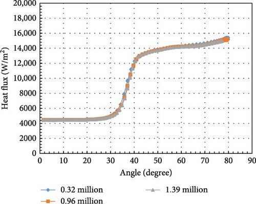
This paper focuses on the LIVE-L7V operating condition, where cooling is applied to both the top and bottom, as illustrated in Figure 10. The radius of the pool is 0.5 m, and the cooling lid is positioned at a height of 41.3 cm [33]. The maximum thermal power of 29 kW in the LIVE-L7V experiment is selected for the simulation. The sidewall temperature is set to 40°C, with a 0.4 mm air gap. At the top of the pool, convective boundary conditions are applied with a convective coefficient of 75 W/m2·K and a freestream temperature of 40°C. At temperatures ranging from 200 to 300°C, the Pr of the mixture of 20% NaNO3-80% KNO3 varies from 6.35 to 10.36. Additional properties of the working fluid are summarized in Table 3 [33, 41]. After comparing temperature and heat flux in Figures 11 and 12, the hexahedral mesh including 1.38 million cells with first layer thickness below 0.1 mm is preferred.
| Symbol | Parameter name | Unit | At the temperature of °C | ||||
|---|---|---|---|---|---|---|---|
| <224 | 284 | 300 | 350 | 400 | |||
| ρ | Density | kg/m3 | 2,200 | 1914 | 1902 | 1866 | 1802 |
| Cp | Specific heat | J/kg·K | 0.9474 + 1.13E−03 T | 1328 | 1332 | 1346 | 1360 |
| λ | Thermal conductivity | W/m·K | 0.4–0.6 | 0.6 | 0.439 | 0.422 | 0.422 |
| μ | Viscosity | kg/m·s | — | 3.77E−03 | 3.33E−03 | 2.52E−03 | 1.93E−03 |
| Pr | Prandtl number | — | — | 8.35 | 10.36 | 8.18 | 6.33 |
| β | Thermal expansion coefficient | 1/K | 3.81E−04 | ||||
| Solidus/liquidus point | °C | 224/284 | |||||
| Pure solvent melting heat | J/kg | 1.62E + 05 | |||||
4.3. Simulation Results
To examine the impact of turbulence models on the computation of the 3D hemisphere melt pool, six turbulence models are utilized to simulate the LIVE-L7V experiment. Notably, the convergence difficulty of the RSM-BSL model is substantial, so the GEKO option is additionally enabled.
4.3.1. Temperature Distribution
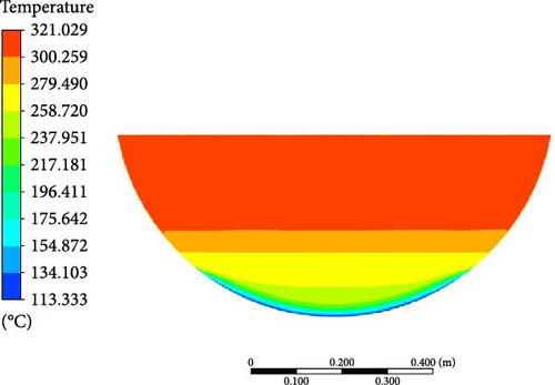
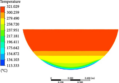
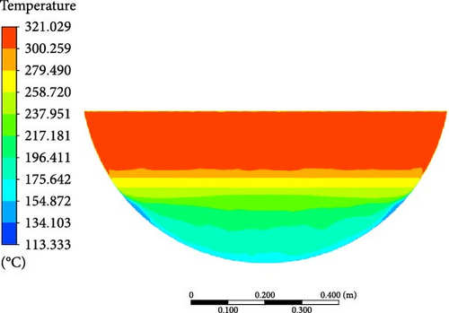
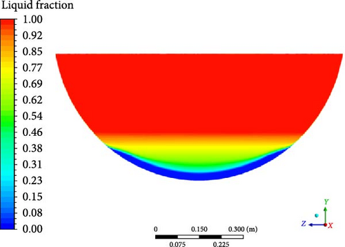
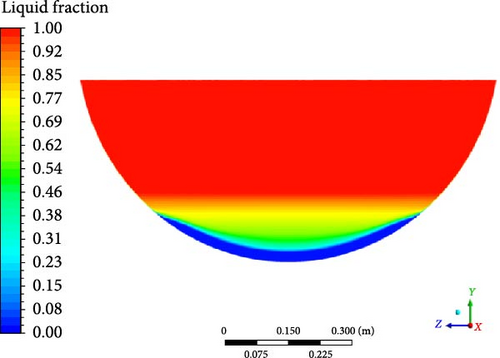
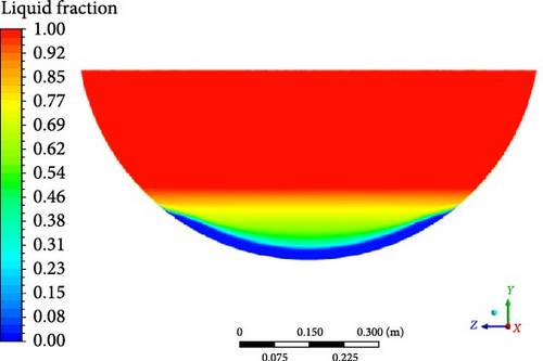
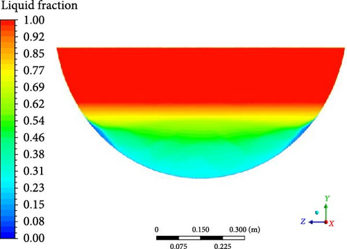
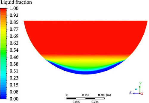
As can be seen from Figure 13, the melt pool temperature distributions from all the turbulence models can be divided into three regions: rapid increase in the crust region, gradual rise in the stably stratified region, and comparatively uniform in the upper region. The stable stratified region consists of both the mushy zone (t < 284°C) and the liquid phase zone (t > 284°C). The slope of temperature increase in the liquid phase zone becomes slightly steeper than the mushy zone. In contrast to the results from other turbulence models, the DES model predicts a smaller temperature range. When comparing the simulation results with the experimental data, it is observed that a higher temperature is evident at the bottom region in the experiment. This may be due to the thermocouples close to the electrical resistance heating wires during the experiment.
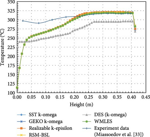
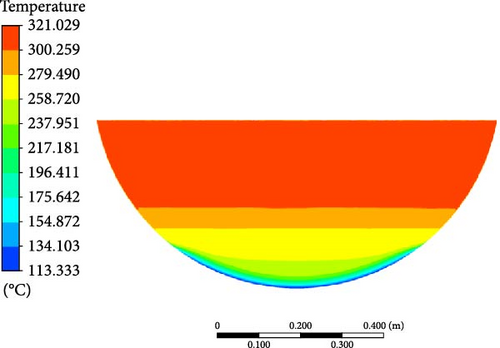
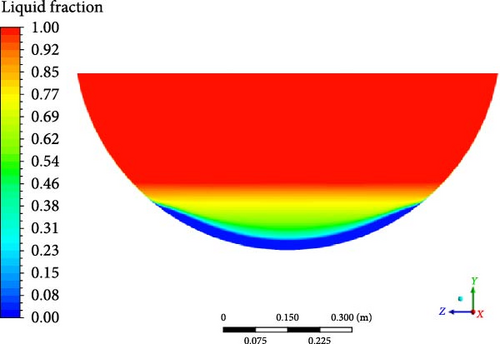
Except for the DES model, the computed melt pool temperature distributions are relatively similar across various turbulence models in Figure 14, with the formation of a stable crust observed at the bottom in Figure 15. When compared to the computational results of other turbulence models, the melt pool crust region (t < 224°C) in the DES simulation is significantly smaller. As a consequence of the limited crust region, a lower temperature is observed in the lower part, while the upper high-temperature zone in the DES model is characterized by a smaller size and lower temperature compared to other turbulence models.


4.3.2. Velocity Distribution
In Figure 16, the velocity distribution within the melt pool can also be classified into three regions: a turbulent mixing region at the top, a downward flow along the sidewalls, and a lateral flow region at the bottom. The downward flow along the sidewalls is a crucial characteristic of natural convection. In the turbulent mixing region at the top, DES and WMLES show the most eddies, leading to more intricate flow patterns. In the lateral flow region at the bottom, DES simulations exhibit the weakest lateral flows among all the models.
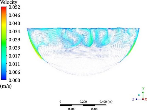
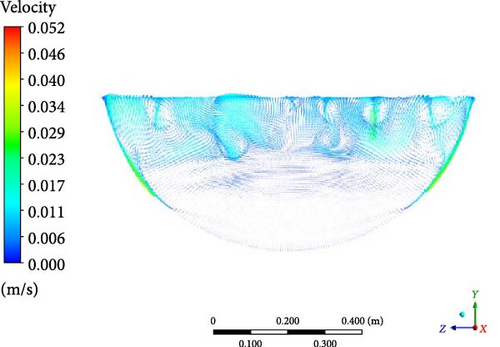
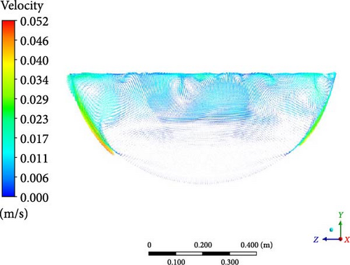
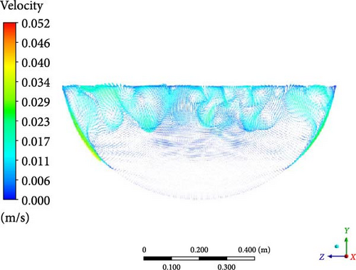
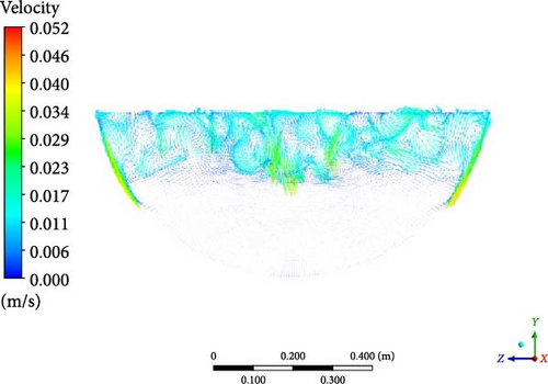
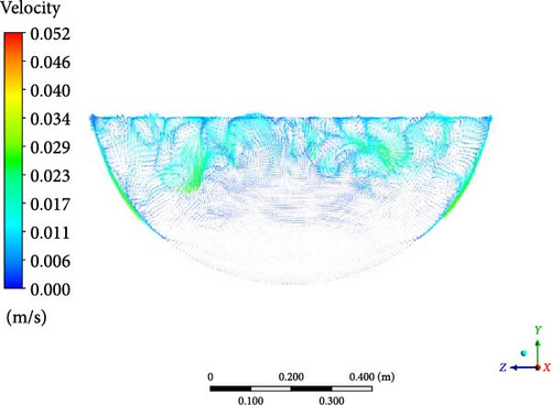
By examining the temperature and velocity, the close relationship between the flow and heat transfer characteristics is also found within the LIVE-L7V experiment. The turbulent mixing region at the top aligns with the uniform temperature region, while the termination point of the downward sidewall flow corresponds to the crust formation boundary. The subtle lateral flow (resulting from low temperature) at the bottom contributes to temperature stratification, while the intense downward flow along the sidewalls creates local overtemperature at the near-wall region.
4.3.3. Heat Flux Distribution
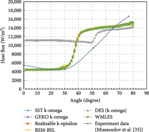
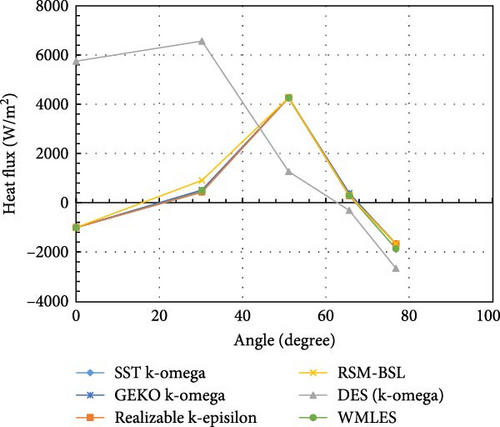
As illustrated in Figure 17, there is minimal variation of the heat flux at the bottom and top and a noticeable increase in the middle region. The limited heat flux at the bottom primarily arises from low temperatures and crust formation, which impedes heat transfer. The heat flux at the top region and middle region respectively corresponds to the uniform high-temperature region and the crustless area. Compared with other models, the DES model exhibits a higher temperature at the bottom and a smaller temperature difference between the top and bottom, which leads to a higher value of heat flux at the bottom and a relatively smaller rise of heat flux in the middle region.
4.4. Comparison With Experimental Data
The flow and heat transfer experimental data show poorer agreement with the DES model compared to the temperature and heat flux results, as demonstrated by the absolute and relative results in Figures 18 and 19, Tables 4 and 5. In other words, DES is not recommended in the LIVE-L7V simulation. In addition, the RSM model is also not recommended because it is extremely difficult to converge in the calculation. In 2D flows, it requires five additional transport equations, while in 3D, seven equations are solved. The RSM is particularly effective in situations where turbulence anisotropy has a significant impact on the mean flow, such as highly swirling flows and stress-driven secondary flows. However, in the calculation of the melt pool, the outstanding advantages of the RSM model are not observed.

| Height (m) | SST k-omega (%) | GEKO k-omega (%) | Realizable k-episilon (%) | RSM-BSL (%) | DES (k-omega) (%) | WMLES (%) |
|---|---|---|---|---|---|---|
| 0.02 | −21.91 | −21.91 | −21.91 | −21.91 | −19.22 | −21.91 |
| 0.08 | −10.28 | −10.28 | −10.28 | −10.28 | −15.44 | −10.28 |
| 0.12 | −8.63 | −8.63 | −8.63 | −8.63 | −15.30 | −8.63 |
| 0.17 | −6.05 | −6.05 | −6.05 | −6.37 | −15.15 | −6.37 |
| 0.22 | −0.30 | −0.30 | 0.99 | 0.02 | −10.62 | −0.62 |
| 0.27 | 1.17 | 1.49 | 1.17 | 1.17 | −7.39 | 0.54 |
| 0.32 | 1.18 | 1.18 | 1.18 | 0.86 | −7.02 | 0.55 |
| 0.37 | 1.36 | 1.36 | 1.36 | 1.04 | −6.85 | 0.41 |
| 0.39 | 1.19 | 1.19 | 0.87 | 0.56 | −6.69 | 0.56 |
| 0.4 | 0.96 | 0.65 | 0.65 | 0.33 | −6.90 | 0.02 |
- Abbreviations: DES, detached eddy simulation; GEKO, generalized k-omega; SST, shear–stress transport; WMLES, wall-modeled large eddy simulation.
| Angle (degree) | SST k-omega (%) | GEKO k-omega (%) | Realizable k-episilon (%) | RSM-BSL (%) | DES (k-omega) (%) | WMLES (%) |
|---|---|---|---|---|---|---|
| 0 | −18.52 | −18.52 | −18.52 | −18.52 | 105.53 | −18.52 |
| 30.24 | 9.41 | 11.39 | 9.63 | 19.99 | 144.84 | 10.73 |
| 51.07 | 45.20 | 45.20 | 45.20 | 45.20 | 13.41 | 45.20 |
| 65.63 | 2.06 | 2.77 | 2.06 | 2.06 | −2.22 | 2.06 |
| 76.85 | −10.00 | −10.00 | −10.00 | −10.00 | −16.00 | −11.20 |
- Abbreviations: DES, detached eddy simulation; GEKO, generalized k-omega; SST, shear–stress transport; WMLES, wall-modeled large eddy simulation.
5. Experiment 3: BALI Experimental Simulation
5.1. Experimental Overview
The BALI experiment explored natural convection heat transfer in a quarter-circle pool, scaled at a 1:1 ratio to represent the lower head of a real RPV, resulting in a Rayleigh number of approximately 1016 [9, 42]. The pool had a 2 m radius and a 0.15 m thickness, as shown in Figure 20, using salt water (with a Prandtl number around 7) as the simulant material. Thermal power was supplied by electrode heating. The top surface had either adiabatic or cooling boundary conditions, while all the vertical walls were adiabatic. The curved wall and the top surface (in the case of top cooling) were cooled using organic fluids at low temperatures (−50 to −80°C). Thermocouples were installed 10 cm from the vertical side wall to measure the temperature distribution, and the heat flux across the curved wall was calculated from temperature differences obtained with the thermocouples.
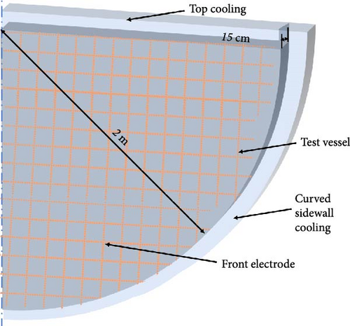
5.2. Simulation Setup
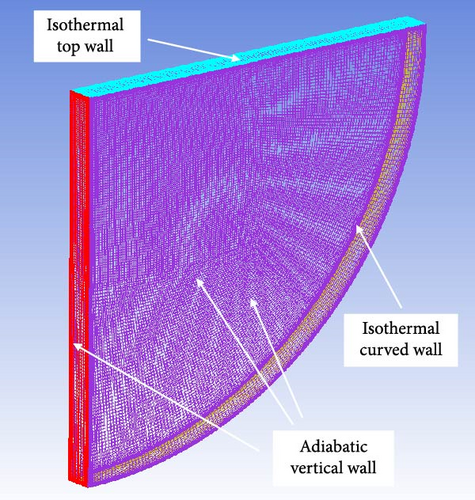
In this analysis, we consider a top cooling scenario with a thermal power input of 15.7 kW. Accordingly, the curved sidewall and top boundary are set to isothermal conditions in the simulation, as shown in Figure 21, while the front and back planes, as well as the vertical sidewalls, are adiabatic. Mesh refinement is performed near the wall at each boundary in Figure 21. The physical properties of salt water are listed in Table 6. The density of water is set using the Boussinesq model.
| Symbol | Parameter name | Unit | Value |
|---|---|---|---|
| ρ | Reference density | kg/m3 | 998.2 |
| Cp | Specific heat capacity | J/kg·K | 4182 |
| λ | Thermal conductivity | W/m·K | 0.6 |
| μ | Viscosity | kg/m·s | 1.00E−03 |
| β | Thermal expansion coefficient | 1/K | 2.07E−04 |
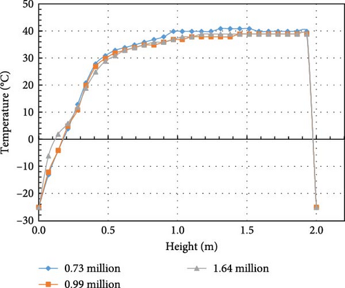
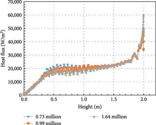
Figures 22 and 23 show how temperature and heat flux vary with height for different grid configurations, using the k-omega SST turbulence model. The temperature data are taken at a position 10 cm from the vertical wall, matching the experimental setup. In all simulations, the first layer thickness meets the requirement of y+ < 1. Comparing the results of the three mesh groups, the temperature results for the 0.99 million and 1.64 million mesh are quite similar, while the heat flux results vary with time but show little overall difference. Based on these simulation results, a mesh size of 0.99 million elements is chosen for the BALI experiment simulations.
5.2.1. Boundary Conditions
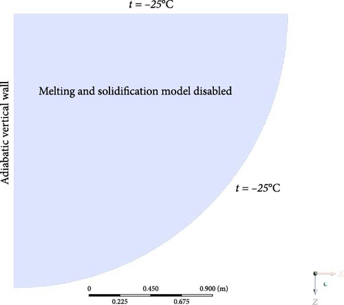
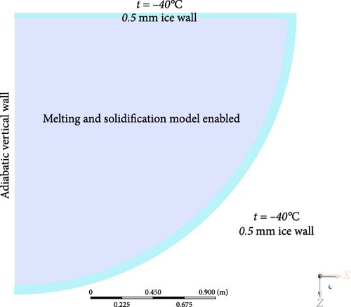
Due to the high Rayleigh number, two types of boundary conditions are employed in the simulation of the BALI experiment, as depicted in Figures 24 and 25:
- 1.
Boundary condition A: the solidification and melting model is not activated, and all the constant temperature boundary is set to −25°C.
- 2.
Boundary condition B: the solidification and melting model is activated, and all the constant temperature boundary is set to −40°C with 0.5 mm ice wall.
In boundary condition A, the formation of an ice crust at the bottom is not taken into account in order to focus on single-phase computations. This simplification of boundary conditions has been commonly used in previous simulations [27, 30]. The curved wall, as well as the bottom and top walls, is all set to a constant temperature of −25°C due to the lowest temperature in the experiment result. In boundary condition B, the solidification and melting are considered. According to the experimental description, organic fluid flows through the cooling curved pipe along the sidewall, cooled by liquid nitrogen at temperatures ranging from −50 to −80°C, leading to ice formation inside the pipe. Therefore, the boundary temperature is set to −40°C, with a 0.5 mm ice layer. Simulations of the BALI experiment were conducted under both boundary conditions, and the results were compared across different turbulence models.
5.3. Simulation Results (Boundary Condition A)
5.3.1. Temperature Distribution
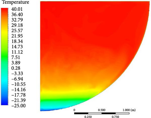
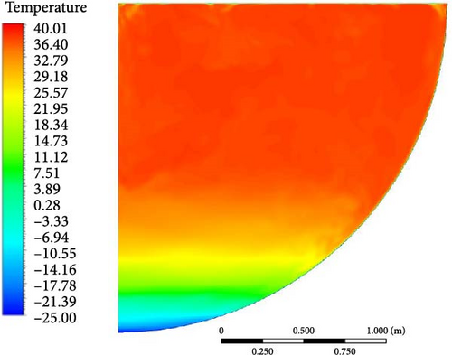
Under boundary condition A, Figure 26 displays the diverse temperature contours of the BALI top cooling experiment across various turbulence models. Similar to the vertical temperature profile of the BALI experiment [9], the temperature at the upper unstable zone remains uniform, and the temperature at the lower stratified zone increases with height. The top cooling boundary causes the formation of a large upper uniform high-temperature zone. At the same height, it is observed that the temperature in the near-wall region is higher than the far-wall region temperature, which can be attributed to the downward flow near the curved sidewall.
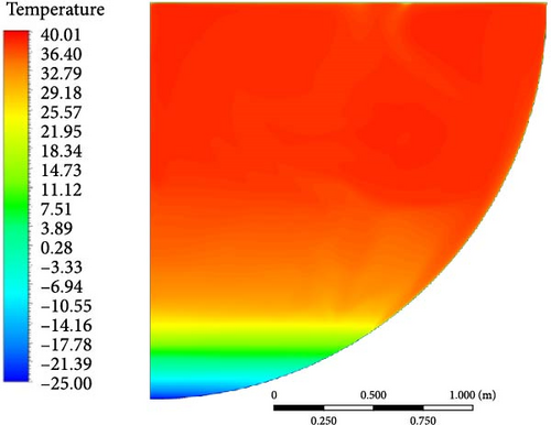
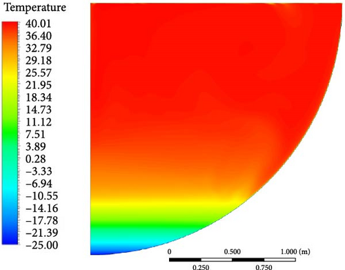
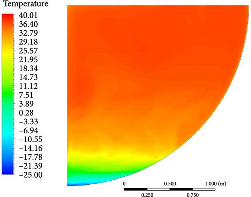
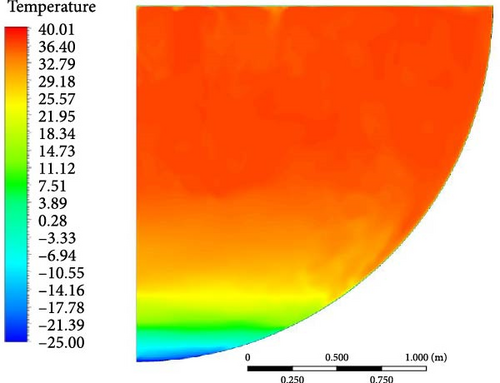
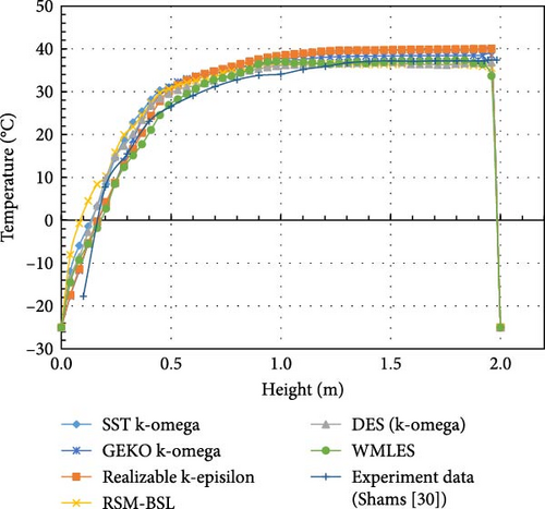
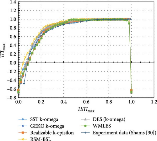
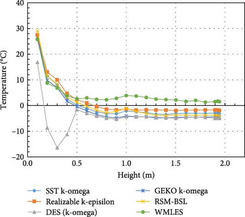
Comparing the calculation results of various turbulence models with the experimental findings [43] in Figure 27, the temperature distribution produced by different turbulence models is roughly in a line. Comparing the “turning point” from the top isothermal region to where the temperature starts to drop, the WMLES model is closer to the experimental results compared to other models, while the RSM-BSL model shows significantly higher temperatures near the bottom. In Figure 28, the uniform temperature distribution curves show that the WMLES and realizable k-epsilon models have overall temperature distributions that are more similar to the experimental results, followed by the SST/GEKO k-omega and DES (k-omega) models, with the RSM-BSL model deviating the most.
5.3.2. Velocity Distribution
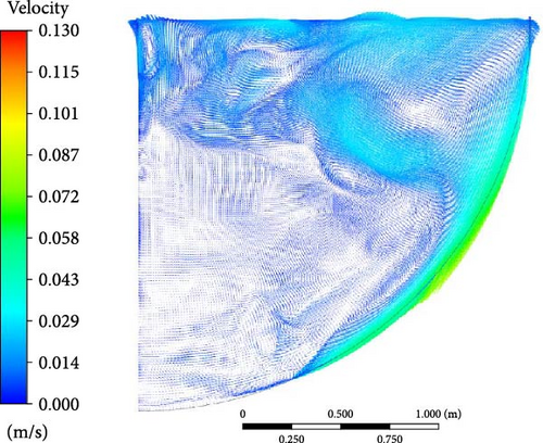
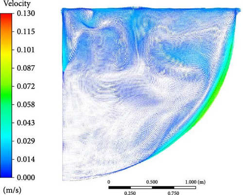
As shown in Figure 29, although the velocity vector varies with time, the downward flow pattern along the curved wall, the flow separation phenomenon, the lateral flow in the bottom, and the upper turbulent mixing region remain stable due to the influence of natural convection. (1) The maximum velocity consistently appears along the downward direction of the curved wall because of the internal heat and sidewall cooling. (2) The combination of the upward trend at the bottom and the downward flow results in flow separation, which leads to a gradual weakening of the downward flow. (3) Low-speed lateral flow occurs at the bottom, with varying magnitude and direction, owing to the minor temperature difference and weak natural convection at the bottom. (4) At the top region, water flows more violently, and eddies are produced because of the natural convection and temperature differences between the pool and the top cooling boundary.
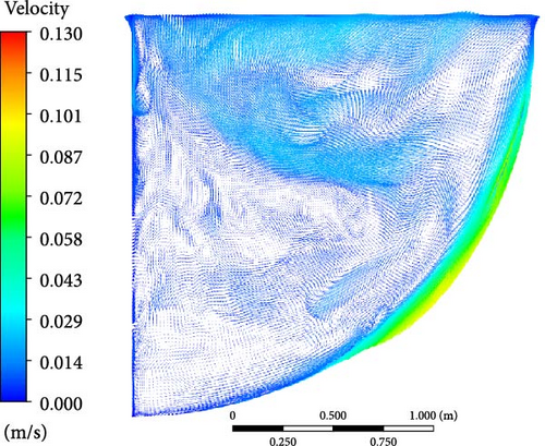
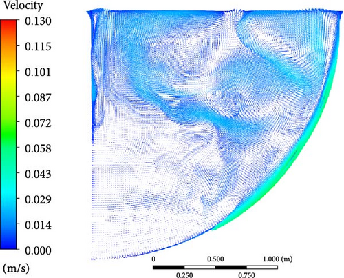
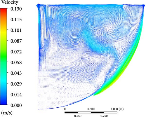
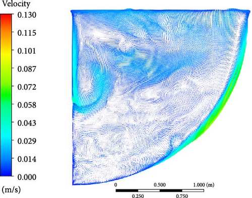
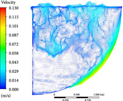
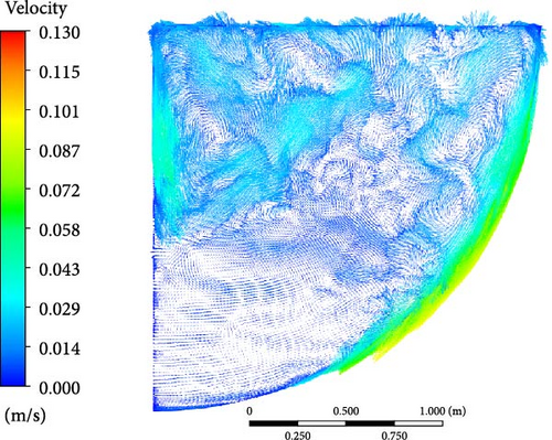
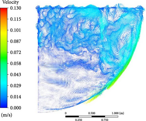
However, the flow characteristics of different turbulence models are slightly different. The WMLES and DES velocity contours, compared with the RANS models, capture more details of the eddies. The upper region is characterized by the presence of numerous small-scale eddies. The downward flow along the side wall undergoes continuous separation, resulting in the formation of multiple small eddies simultaneously. These small eddies tend to merge and form larger eddies. Macroscopically, multiple eddies can be observed at the top, with their direction, shape, and number changing over time, similar to the RANS velocity contours.
Combining the temperature and velocity plots, the turbulent mixing region at the top coincides with the uniform temperature region, while the horizontal flow region overlaps with the gradually increasing temperature region at the bottom. In addition, the downward flow along the sidewall causes a local temperature increase at the edge of the sidewall.
5.3.3. Heat Flux Distribution
In Figure 30, the highest heat flux is observed in the top region of the simulation result. This can be attributed to the isothermal cooling boundary condition, which results in low velocity near the side wall and flow stagnation, creating a “blind area” with restricted flow. Consequently, the heat flux in this region increases sharply. Especially in this case, where both the top and side walls are being cooled simultaneously, the flow in the corner “blind zone” is weakened, further intensifying the peak heat flow observed at the top.
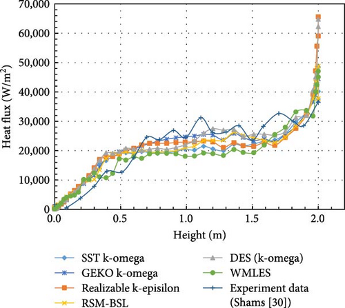
There are some variations in the heat flux results from different turbulence models, considering the flowing and roiling in natural convection, the heat flux distribution produced by different turbulence models is roughly in a line, as shown in Figure 31.
5.4. Simulation Results (Boundary Condition B)
5.4.1. Temperature Distribution
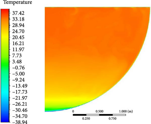
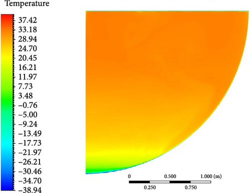
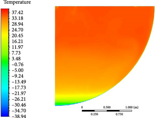
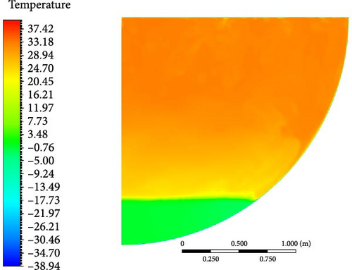
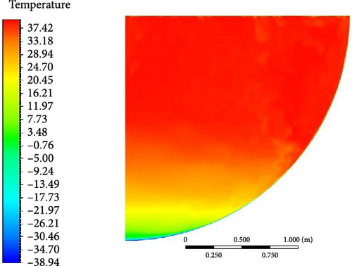
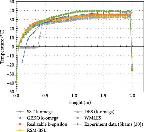
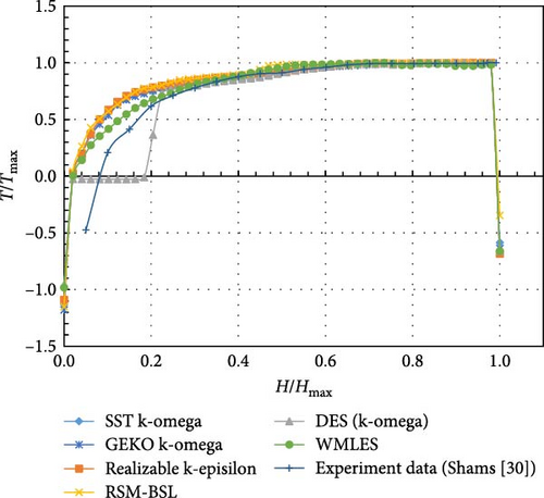
In analyzing the temperature distribution from the different turbulence models and their comparison with experimental data in Figures 32–34, several trends can be observed:

- 1.
WMLES model: The WMLES model shows the closest agreement with experimental data across the entire height of the domain. It matches the temperature distribution curve, particularly near the top region where the transition occurs from isothermal to lower temperatures. The WMLES model’s performance is also evident in the normalized temperature graph, where it follows the experimental curve closely, indicating an accurate prediction of both the turning point and the lower regions of the domain.
- 2.
DES (k-omega): The DES model shows significant deviations from the experimental data, especially near the bottom and in the transition region. Its performance is the least accurate among the models, especially in capturing the turning point and lower temperature regions. It tends to predict much lower temperatures, and the gradient of the temperature drop is more abrupt than what is observed experimentally. The bottom region is shown as a solid phase in Figure 35. In the normalized graph, this model exhibits a similar trend, with a larger deviation from the experimental curve in the lower regions.
- 3.
Other models: In the temperature distributions of the other turbulence models, a significant degree of similarity is observed overall. Whether it is the SST k-omega, GEKO k-omega, RSM-BSL, or realizable k-epsilon model, the temperature contours exhibit smooth gradients, with temperatures increasing gradually from the colder region at the bottom to higher values, especially near the upper area where the temperature changes become more stable. These models show consistency in capturing the large-scale vortices in natural convection, with the heat transfer process displaying similar characteristics and relatively uniform temperature distributions. These models perform reasonably well in the middle region, though their deviation becomes more pronounced in the bottom region, showing higher temperatures compared to the experimental results.
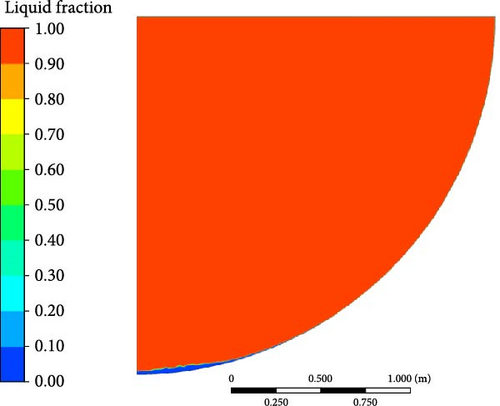
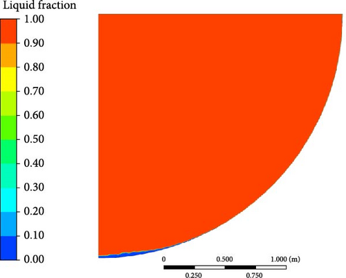
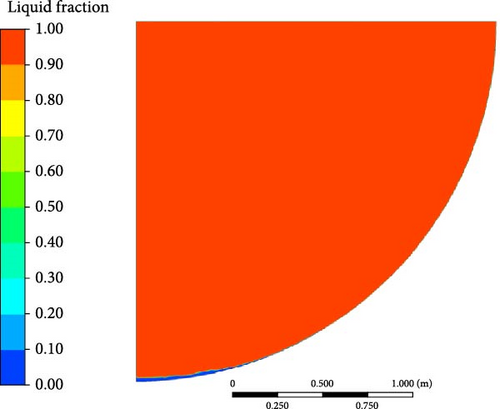

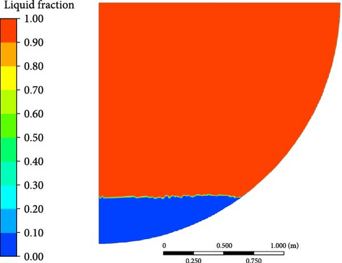
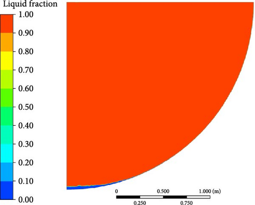
To summarize, The WMLES model provides the best match to experimental data, particularly in capturing the overall temperature distribution and the turning point. DES (k-omega) exhibits significant deviations, particularly in the lower regions, making them less accurate for this specific case. Other turbulence models perform moderately well, though they show slight overpredictions at the turning point.
5.4.2. Velocity Distribution
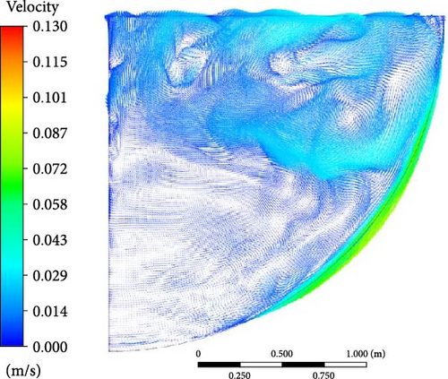
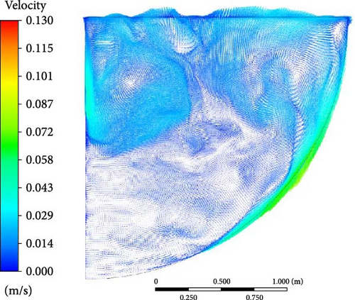
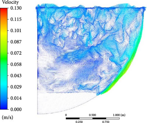
Similar to boundary condition A, in the comparison of flow characteristics across different turbulence models in Figure 36, the WMLES and DES models capture more details in the velocity profiles compared to RANS. However, in the DES model, due to a thicker ice formation zone at the bottom, the descending flow is halted by the solid region, resulting in a smaller lateral flow area at the bottom.
5.4.3. Heat Flux Distribution
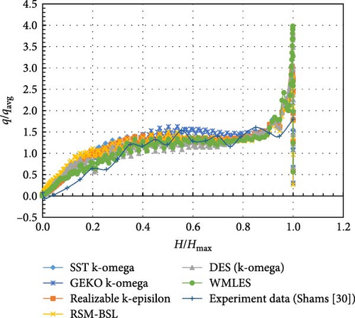
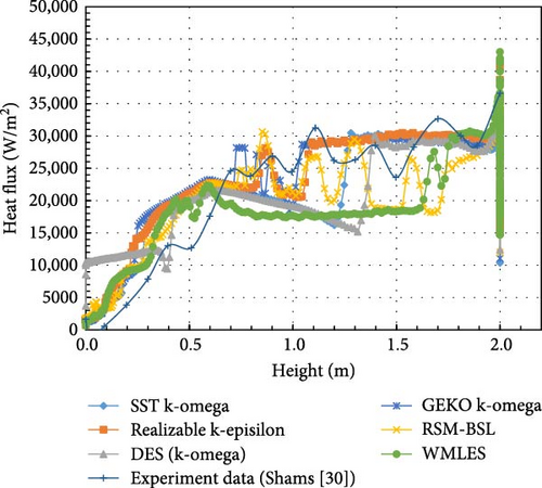
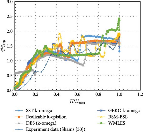
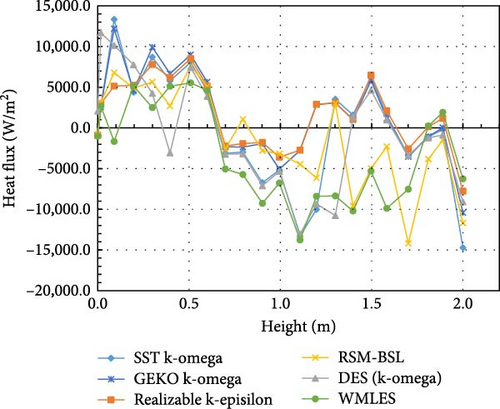
Due to crust formation on the sidewalls, the heat flux distribution in Figure 37 is no longer as uniform as in boundary condition A, as in Figure 30. The heat flux in the DES and SST models shows a noticeable downward trend in the middle, resulting in some discrepancies with the experimental data. The RSM-BSL model exhibits the largest fluctuations in heat flux, resembling the experimental results, while the realizable k-epsilon and GEKO k-omega models also show significant fluctuations. When the local heat flux is normalized by the average heat flux in Figure 38, the distribution from the RSM-BSL model is closest to the experimental data, with the WMLES, realizable k-epsilon, and GEKO k-omega models also being relatively close.
5.5. Comparison With Experimental Data
Based on the values obtained from the experiment and the simulation results of various turbulence models at corresponding experimental measurement positions, the absolute error was calculated to evaluate the accuracy of each turbulence model.
First, the absolute errors of temperature and heat flux in the BALI simulation of different turbulent models under boundary condition A are calculated, as illustrated in Figures 39 and 40. Given the high Rayleigh number in the BALI experiment and the favorable fluid flow properties of water, the results from various turbulence models exhibit considerable fluctuations, yet still maintain a consistent overall pattern in temperature and heat flux distribution. The results from each turbulence model are generally consistent, showing minimal differences in error. However, the RSM-BSL model exhibits the most notable deviation in the bottom region. This suggests that while all turbulence models can effectively simulate high Rayleigh number natural convection, the RSM-BSL model’s unique behavior underscores its sensitivity to flow characteristics, leading to less accurate predictions of flow and heat transfer compared to the other models, particularly in the absence of crust formation in boundary condition A.
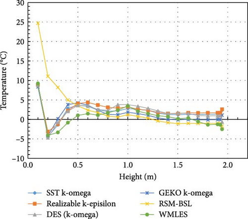
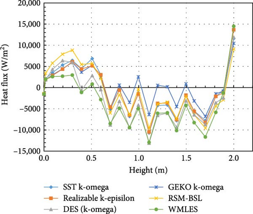
Then, in comparison of wall boundary condition B which includes solidification and melting in Figure 41, it is observed that the DES model shows a significant deviation in bottom temperature, while the WMLES model tends to overestimate temperature at the upper region, and the other models generally underestimate it. The absolute temperature errors of turbulence models at various heights under conditions A and B are shown in Table 7. Regarding heat flux in Figure 42, due to the substantial fluctuations, the absolute differences still yield limited conclusions. The absolute heat flux errors of turbulence models at various heights under conditions A and B are presented in Table 8. Based on the earlier analysis of normalized temperature results, the WMLES model aligns most closely with the experimental data. In contrast, the DES (k-omega) model demonstrates considerable deviations, particularly in the lower regions. As for the normalized heat flux, the RSM-BSL model shows the best agreement with the experimental data, while the WMLES, realizable k-epsilon, and GEKO k-omega models also yield relatively comparable results.
| Height (m) | SST k-omega | GEKO k-omega | Realizable k-episilon | RSM-BSL | DES (k-omega) | WMLES | ||||||
|---|---|---|---|---|---|---|---|---|---|---|---|---|
| A | B | A | B | A | B | A | B | A | B | A | B | |
| 0.1 | 9.09 | 27.44 | 8.36 | 26.74 | 8.84 | 27.48 | 24.71 | 29.07 | 8.81 | 16.88 | 9.25 | 25.73 |
| 0.2 | −4.44 | 11.44 | −4.21 | 9.84 | −3.14 | 13.04 | 11.07 | 11.44 | −4.68 | −8.67 | −4.11 | 8.74 |
| 0.3 | −1.4 | 8.18 | 0.13 | 6.94 | −1.23 | 10.01 | 8.23 | 8.35 | −0.73 | −16.39 | −3.33 | 6.85 |
| 0.4 | 2.86 | 2.5 | 3.8 | 1.7 | 2.27 | 4.7 | 4.99 | 3.2 | 2.09 | −11.2 | −0.83 | 3.8 |
| 0.5 | 3.64 | 0.22 | 4.24 | −0.4 | 4.09 | 2.32 | 3.51 | 1.27 | 3.63 | −1.58 | 1.04 | 2.62 |
| 0.6 | 3.36 | −1.12 | 3.67 | −2.09 | 4.37 | 0.98 | 2.37 | −0.26 | 3.49 | −3.02 | 1.47 | 2.98 |
| 0.7 | 2.43 | −2.44 | 2.34 | −3.47 | 3.7 | −0.37 | 1.74 | −1.77 | 2.54 | −4.06 | 1.09 | 2.39 |
| 0.8 | 2.06 | −3.16 | 1.29 | −4.42 | 3.1 | −1.42 | 0.86 | −2.84 | 2.31 | −4.92 | 1.69 | 2.26 |
| 0.9 | 2.2 | −3.2 | 1.2 | −4.8 | 2.9 | −1.7 | 0.6 | −2.3 | 3.8 | −5.3 | 2.4 | 2.8 |
| 1 | 2.78 | −2.1 | 1.83 | −4.1 | 3.24 | −1.35 | 1.22 | −1.15 | 3.78 | −4.35 | 3.44 | 3.9 |
| 1.1 | 2.59 | −2.4 | 1.49 | −4.3 | 2.59 | −1.8 | 0.79 | −2.3 | 3.4 | −4.4 | 2.1 | 3.7 |
| 1.2 | 2.34 | −2.75 | 1.04 | −4.35 | 2.33 | −1.65 | 0.34 | −3.1 | 2.84 | −4.35 | 1.5 | 3.15 |
| 1.3 | 1.6 | −3.33 | 0.39 | −4.83 | 1.79 | −1.75 | −0.4 | −3.8 | 2.19 | −4.45 | 0.96 | 2.53 |
| 1.4 | 1.23 | −3.45 | 0 | −4.78 | 1.5 | −1.78 | −0.83 | −3.85 | 1.47 | −4.8 | 0.7 | 2.33 |
| 1.5 | 1.2 | −3.13 | −0.1 | −4.63 | 1.48 | −1.95 | −1.08 | −3.73 | 1.62 | −4.93 | 0.16 | 2.18 |
| 1.61 | 1.3 | −3 | 0 | −4.5 | 1.7 | −1.8 | −1 | −3.7 | 1.53 | −4.6 | 0.37 | 1.6 |
| 1.7 | 1.27 | −3 | −0.1 | −4.5 | 1.67 | −1.8 | −1.03 | −3.8 | 1 | −4.5 | −0.57 | 2 |
| 1.8 | 1.3 | −3 | −0.1 | −4.5 | 1.7 | −1.7 | −1 | −3.7 | 0.9 | −4.6 | −1.37 | 1.3 |
| 1.9 | 1.35 | −2.95 | −0.05 | −4.4 | 1.7 | −1.7 | −1 | −3.8 | 0.95 | −4.95 | −1.26 | 1.5 |
| 1.93 | 1.39 | −2.9 | −0.01 | −4.4 | 1.7 | −1.7 | −1 | −3.8 | 0.99 | −4.9 | −1.38 | 1.7 |
| 1.94 | 2.36 | −3.1 | 1.1 | −4.6 | 2.6 | −1.9 | −1.73 | −4.17 | −0.64 | −4.93 | −2.51 | 1.5 |
- Abbreviations: DES, detached eddy simulation; GEKO, generalized k-omega; SST, shear–stress transport; WMLES, wall-modeled large eddy simulation.
| Height (m) | SST k-omega | GEKO k-omega | Realizable k-episilon | RSM-BSL | DES (k-omega) | WMLES | ||||||
|---|---|---|---|---|---|---|---|---|---|---|---|---|
| A | B | A | B | A | B | A | B | A | B | A | B | |
| 0.0 | −1412 | −915 | −1547 | −892 | −1546 | −930 | −1422 | −773 | −1507 | 2075 | −1526 | −1026 |
| 0.0 | 2157 | 2555 | 1866 | 2575 | 1840 | 2992 | 3401 | 3116 | 1858 | 11,684 | 1960 | 2688 |
| 0.1 | 3508 | 13,348 | 3003 | 12,183 | 2865 | 5133 | 5792 | 6788 | 4311 | 10,132 | 2592 | −1668 |
| 0.2 | 5343 | 4387 | 4437 | 4557 | 4370 | 5245 | 7896 | 4883 | 6386 | 7760 | 2700 | 5176 |
| 0.3 | 6423 | 8703 | 5965 | 9921 | 6090 | 7791 | 8838 | 5646 | 5934 | 4248 | 2955 | 2494 |
| 0.4 | 4479 | 5789 | 3651 | 6670 | 4399 | 6206 | 5466 | 2694 | −605 | −3067 | −1142 | 5123 |
| 0.5 | 6859 | 8043 | 5295 | 8988 | 5177 | 8516 | 5698 | 7616 | 2852 | 7421 | 840 | 5538 |
| 0.6 | 3048 | 4619 | 2424 | 5649 | 3027 | 5167 | 2160 | 5115 | −454 | 3872 | −2825 | 4629 |
| 0.7 | −5165 | −3122 | −4851 | −2316 | −4586 | −2222 | −5982 | −2568 | −8793 | −3236 | −8500 | −5050 |
| 0.8 | −384 | −2963 | 589 | −2351 | −583 | −1922 | −1655 | 1065 | −3205 | −3185 | −4867 | −5730 |
| 0.9 | −6793 | −6727 | −3486 | −1940 | −6456 | −1777 | −6419 | −2798 | −9440 | −7106 | −9418 | −9270 |
| 1.0 | −1255 | −5167 | 2549 | −5062 | −1480 | −3595 | −338 | −3178 | −4124 | −5343 | −4949 | −6775 |
| 1.1 | −10,693 | −13,292 | −6374 | −2767 | −10471 | −2724 | −9569 | −4453 | −13,101 | −13,053 | −12,926 | −13,766 |
| 1.2 | −4233 | −10,026 | 547 | 2854 | −3742 | 2904 | −3878 | −6135 | −6542 | −9341 | −6059 | −8399 |
| 1.3 | −4105 | 3529 | 200 | 3080 | −3627 | 3077 | −3428 | 3006 | −6027 | −10,769 | −5940 | −8362 |
| 1.4 | −7807 | 1594 | −4477 | 998 | −7531 | 1073 | −7313 | −9602 | −9360 | 1352 | −10,146 | −10,210 |
| 1.5 | −1855 | 6232 | 888 | 5829 | −1793 | 6480 | −2072 | −4991 | −3099 | 4626 | −4209 | −5312 |
| 1.6 | −5508 | 1555 | −3142 | 1179 | −5611 | 2117 | −6422 | −2291 | −6405 | 974 | −8265 | −9883 |
| 1.7 | −7779 | −3401 | −6800 | −3548 | −8230 | −2580 | −9567 | −14,198 | −8701 | −3373 | −11,654 | −7533 |
| 1.8 | −2033 | −1106 | −1458 | −1055 | −2051 | 150 | −4338 | −3829 | −3572 | −1234 | −5846 | 238 |
| 1.9 | −750 | −192 | −830 | 30 | −1252 | 1171 | −2889 | −1498 | −2391 | −859 | −1257 | 1918 |
| 2.0 | 11,585 | −14,728 | 10,453 | −10,417 | 13,659 | −7774 | 9103 | −11,674 | 11,931 | −9081 | 14,494 | −6255 |
- Abbreviations: DES, detached eddy simulation; GEKO, generalized k-omega; SST, shear–stress transport; WMLES, wall-modeled large eddy simulation.
6. Discussion
6.1. Comparative Analysis
When comparing the results of all three experiments and simulations, it is evident that despite variations in shape, materials, and boundary conditions, the differences among turbulence models become increasingly pronounced with rising Rayleigh numbers. Notably, the applicability of the DES model to solidification and melting processes has certain limitations.
In the case of the BALI experiment, direct simulation of solidification and melting is rarely employed due to the high Rayleigh number increasing significantly with height, leading to stricter requirements for boundary layer mesh refinement and other parameters in natural convection scenarios with internal heat sources. In contrast, the 3D horizontal rectangular configuration at low Rayleigh numbers and without solidification and melting boundaries presents a much lower convergence difficulty, choosing turbulence models less critical.
6.2. Insights on Boundary Conditions
Overall, the influence of boundary conditions, particularly in the BALI experiment, highlights their critical role in shaping the behavior and accuracy of turbulence models. The solidification and melting processes introduce additional challenges for simulation fidelity. In the BALI experiment, the two boundary conditions have a significant impact on the simulation results and their alignment with experimental data. Analyzing these effects reveals how different boundary conditions can lead to variations in model performance and affect the overall reliability of the simulations.
In comparing boundary conditions A and B, the most significant difference is the noticeable crust formation at the bottom in the DES model, which has a clear impact on temperature, solid–liquid distribution, and velocity. Additionally, the solidification and melting processes also significantly affect heat transfer to the sidewalls, leading to greater differences between the results of the various turbulence models.
6.3. Limitations and Model Assumptions
- 1.
Limitations of the turbulence model: The DES model combines LES with RANS equations. Under LRNs or specific flow conditions, the model may not accurately capture the characteristics of turbulence, leading to less accurate simulations of flow and heat transfer at the bottom.
- 2.
Interface capture: If the model does not properly handle the phase change interface between solid and liquid, it may lead to inaccurate predictions of temperature distribution in the solid phase. This situation could overlook or underestimate the heat exchange between the liquid and solid phases, thus affecting the temperature prediction at the bottom.
- 3.
Heat transfer mechanisms: The model might not account for certain heat transfer mechanisms in the bottom region (such as natural convection or radiation), which could be more significant in the solid phase, leading to lower temperature prediction at the bottom.
In summary, the combination of these factors may result in inaccurate temperature predictions in the bottom region of the DES model, subsequently affecting the overall simulation of temperature distribution.
7. Conclusions
This study investigated the applicability and accuracy of six commonly used turbulence models in simulating natural convection phenomena relevant to IVR strategies during severe nuclear accidents. By comparing the Kulacki–Goldstein, LIVE-3D, and BALI experiments, we provided insights into the strengths and limitations of each model under different conditions.
Kulacki–Goldstein experiment: All turbulence models demonstrated reliable performance, with simulated temperature ranges aligning well with experimental data. The relative temperature values remained between those from DNS and experimental results, indicating overall reliability (<0.1%). Deviations were minimal, showcasing the selected models’ suitability for scenarios involving simpler geometries and lower Rayleigh numbers.
LIVE-3D experiment: Considering crust formation, the DES model exhibited poor agreement with experimental data, particularly regarding temperature and heat flux. In addition, the RSM-BSL model, while effective in turbulence anisotropy scenarios, struggled with convergence and did not show advantages in melt pool calculations. Thus, neither model is recommended for this type of simulation.
BALI experiment: Simulations were conducted with and without the solidification and melting model, enabling a comparison across different turbulence models. While all models produced satisfactory results for high Rayleigh number natural convection without solidification and melting, the RSM-BSL model showed significant deviations, especially in the bottom region. Considering the crust formation by using the solidification and melting model, the WMLES model matched the distribution of experimental data better, while the RSM-BSL, realizable k-epsilon, and GEKO k-omega models provided comparable results. Notably, the DES model exhibited substantial deviations in bottom temperature under solidification and melting simulation of both LIVE-3D and BALI simulation, manifesting its limitations in accurately modeling the solidification and melting processes in these scenarios.
In summary, the selection of turbulence models should be based on the specific conditions of the simulation. The WMLES model is recommended for its accuracy in predicting temperature distributions, particularly in complex geometries with high Rayleigh numbers. The realizable k-epsilon and GEKO k-omega models are also suitable alternatives due to their reliable performance. Conversely, the RSM model, while valuable in anisotropic turbulence scenarios, may not be ideal for melt pool simulations due to convergence challenges. The DES model also introduces additional deviations in solidification and melting. Future research should focus on refining these models and exploring additional boundary conditions to enhance the accuracy and reliability of predictions in natural convection simulations. Furthermore, it is essential to conduct a thorough investigation into the adaptability of turbulence models across varying melt pool conditions to enhance predictive accuracy.
Conflicts of Interest
The authors declare no conflicts of interest.
Funding
This research was financially supported by the China National Nuclear Corporation (CNNC) under project KY24007 and the National Key R&D Program of China (grant no. 2018YFB1900100).
Appendix
Turbulence Models Used in the Paper
Reynolds-Averaged Navier–Stokes (RANS) turbulence models
These equations are called RANS equations. They have the same general form as the instantaneous Navier–Stokes equations, with the velocities and other solution variables now representing ensemble-averaged (or time-averaged) values. Additional terms now appear that represent the effects of turbulence. These Reynolds stresses, , must be modeled to close the RANS equations.
Eddy-Viscosity Models (EVMs)
Depending on the number of introduced differential equations, the EVMs can be categorized as follows: zero-equation models, one-equation models, two-equation models, etc. In the case of the k-ε and k − ω models, two additional transport equations (for the turbulence kinetic energy, k, and either the turbulence dissipation rate, ε, or the specific dissipation rate, ω) are solved and computed as a function of k and ε or k and ω. The disadvantage of the Boussinesq hypothesis as presented is that it assumes μt is an isotropic scalar quantity, which is not strictly true. However, the assumption of an isotropic turbulent viscosity typically works well for shear flows dominated by only one of the turbulent shear stresses. This covers many technical flows, such as wall boundary layers, mixing layers, jets, and so on.
Realizable k-epsilon turbulence model
Gk represents the generation of turbulence kinetic energy due to the mean velocity gradients; Gb is the generation of turbulence kinetic energy due to buoyancy; YM represents the contribution of the fluctuating dilatation in compressible turbulence to the overall dissipation rate. C2 and C1ε are constants. σk and σε are the turbulent Prandtl numbers for k and ε, respectively. Sk and Sε are user-defined source terms.
The k equation is the same as that in the standard k-ε model and the RNG k-ε model, except for the model constants. The Cμ is no longer constant in realizable k-ε model. However, the form of the ε equation is quite different from those in the standard and RNG-based k-ε models.
Shear-Stress Transport (SST) k-omega turbulence model
Gk represents the production of turbulence kinetic energy; Gω represents the generation of ω; Γk and Γω represent the effective diffusivity of k and ω; Yk and Yω represent the dissipation of k and ω due to turbulence; Dω represents the cross-diffusion term; Sk and Sω are user-defined source terms; and Gb and Gωb account for buoyancy terms.
Generalized k-ω (GEKO) Model
- •
CSEP—parameter to optimize flow separation from smooth surfaces.
- ⚬
0.7 < CSEP < 2.5 (default CSEP = 1.75).
- ⚬
- •
CNW—parameter to optimize flow in nonequilibrium near wall regions (such as heat transfer or Cf).
- ⚬
−2 < CNW < 2 (default CNW = 0.5).
- ⚬
- •
CMIX—parameter to optimize strength of mixing in free shear flows.
- ⚬
0 < CMIX<1 (default: correlation ).
- ⚬
- •
CJET—parameter to optimize free shear layer mixing (optimize free jets independent of mixing layer).
- ⚬
0 < CJET < 1 (default CJET = 0.9).
- ⚬
The model can also be tuned with the curvature correction parameter Ccurv.
Reynolds-Stress Turbulence Model (RSM)
The alternative to the Boussinesq hypothesis, as shown in the RSM, is to solve transport equations for each of the terms in the Reynolds stress tensor. An additional scale-determining equation (normally for ε or ω) is also required. This means that five additional transport equations are required in 2D flows and seven additional transport equations must be solved in 3D.
For the 3D, the exact transport equations for the transport of the Reynolds stresses
The terms on the left of the equation are local time derivative term and convection term Cij separately. The terms on the right of the equation are turbulent diffusion DT,ij, molecular diffusion DL,ij, stress production Pij, buoyancy production Gij, pressure–strain φij, dissipation εij, production by system rotation Fij, and user-defined source term separately.
Detached Eddy Simulation (DES) Model
Large Eddy Simulation (LES) Model
The WMLES model is based on the LES model. In the LES method, a filtering function distinguishes between large and small eddies. Large eddies, which exhibit stronger problem-dependence, are directly resolved using the N–S equation. Meanwhile, common smaller eddies are handled through SGS modeling.
Here, hmax is the maximum edge length of the cell; hwn is the wall normal grid spacing; Cw is constant 0.15.
Open Research
Data Availability Statement
The data that support the findings of this study are available from the corresponding author upon reasonable request.


