A Robust Approach to Extend Deterministic Models for the Quantification of Uncertainty and Comprehensive Evaluation of the Probabilistic Forecasting
Abstract
Forecasting generation and demand forms the foundation of power system planning, operation, and a multitude of decision-making processes. However, traditional deterministic forecasts lack crucial information about uncertainty. With the increasing decentralization of power systems, understanding, and quantifying uncertainty are vital for maintaining resilience. This paper introduces the uncertainty binning method (UBM), a novel approach that extends deterministic models to provide comprehensive probabilistic forecasting and thereby support informed decision-making in energy management. The UBM offers advantages such as simplicity, low data requirements, minimal feature engineering, computational efficiency, adaptability, and ease of implementation. It addresses the demand for reliable and cost-effective energy management system (EMS) solutions in distributed integrated local energy systems, particularly in commercial facilities. To validate its practical applicability, a case study was conducted on an integrated energy system at a logistics facility in northern Germany, focusing on the probabilistic forecasting of electricity demand, heat demand, and PV generation. The results demonstrate the UBM’s high reliability across sectors. However, low sharpness was observed in probabilistic PV generation forecasts, attributed to the low accuracy obtained by the deterministic model. Notably, the accuracy of the deterministic model significantly influences the accuracy of the UBM. Additionally, this paper addresses various challenges in popular evaluation scores for probabilistic forecasting with implementing new ones, namely a graphical calibration score, quantile calibration score (QCS), and percentage quantile calibration score (PQCS). The findings presented in this work contribute significantly to enhancing decision-making capabilities within distributed integrated local energy systems.
1. Introduction
Power systems are undergoing a profound transformation in the form of decentralization, along with the penetration of renewable energy sources, battery electric vehicles (BEVs), heat pumps, hydrogen, etc. This results in increasing uncertainties due to intermittent generation, as well as dynamic and less predictable demand [1–3]. These present challenges to power system planning and operation practices, such as in terms of energy management, economic dispatch, unit commitment, maintenance planning, etc. [4]. Traditional deterministic forecast techniques do not capture uncertainties, which leads to decision-makers being poorly advised [5]. A modern energy system, therefore, requires appropriate quantification of uncertainty to enable informed decision-making. In contrast to deterministic forecasts, the probabilistic forecasting method provides information about uncertainty and should, therefore, be investigated to facilitate the energy transition [6–8]. Following the “Global Energy Forecasting Competitions” in 2012 and 2014 [9, 10], there has been a significant surge in research interest in probabilistic forecasting within the energy domain [10]. With the decentralization of power systems, a growing need has emerged in recent years for quantifying uncertainties in energy management systems (EMSs) within smaller facilities, including residential buildings and small- to medium-sized commercial buildings. These facilities require cost-effective EMS solutions that integrate probabilistic prediction techniques while being simple, convenient, and implementable with minimal data requirements.
Despite the potential benefits of probabilistic forecasting methods in offering uncertainty information, they are complex, data-intensive, and computationally demanding [3]. Additionally, a notable fraction of these methods rely on black-box models, which lack transparency, as highlighted in prior research [11]. Transparency is a crucial attribute in forecasting methodologies [1]. Furthermore, research still leans heavily toward deterministic forecasting [8, 12, 13]. While many probabilistic forecasting models directly generate forecast distributions without tying back to deterministic models, the literature concerning the combination of these approaches remains sparse. Typically, most literature employs the quantile regression averaging (QRA) method, which follows the approach of leveraging deterministic methods. This concept has been applied across various scenarios, including to electricity prices [14–16], electricity load [7, 17], solar PV generation [5], and wind power generation [3, 18]. However, the demand for multiple-point forecast models introduces challenges such as high data requirements, model complexities, and increased computational time. Furthermore, quantile regression (QR) itself demands extensive computational resources, necessitating separate model training for each quantile [19]. If the post-processing method adds significant complexity and effort on top of the development of the deterministic models, its practical value may be undermined.
Wang et al. [7] introduced a probabilistic forecast method that leverages existing point forecast methods by modeling the conditional forecast residual using QR to derive the probabilistic forecasts. Although this approach reduces reliance on multiple-point forecast models, it still necessitates complex post-processing modeling. Another study by Zhang et al. [20] employed copula theory to model the conditional forecast error for stochastic unit commitment in multiple wind farms. Dang et al. [21] utilized point forecasts from three deep neural network models and a similar-day load selection algorithm to facilitate short-term probabilistic load forecasting via quantile random forests (QRFs). Subsequently, QRF found diverse applications across various domains [19, 22–25]. Zhang, Quan, and Srinivasan [3] found QRF to be both more accurate and computationally efficient compared to QRA.
The empirical prediction intervals (EPIs) method, first introduced by William and Goodman [26], produces probabilistic forecasts around existing point forecasts based on the distribution of past point forecast errors within a time window [27]. This method has been implemented in various fields, including meteorology [28], economics [29], and energy [30]. However, the major limitation to EPIs is that the PIs are not conditional [27]. This leads to wider interval width due to unconditional uncertainty, making them less adaptive. Hence, it limits its wider application for decision-making in certain sectors and use cases. To quantify uncertainty in a wind power forecast for a wind farm in China, Huang et al. [31] presented a simplistic statistical approach that transforms point forecasts into interval forecasts by considering the conditional dependence between predicted values and prediction errors. Saber [32] then proposed three methods to transform point forecasts into probabilistic ones with relative ease of implementation. Compared to Huang et al. [31], Saber’s methods employed historical weather data as conditionals. Saber’s approach finds application in the quantification of uncertainties in U.S. electricity and natural gas consumption. Nevertheless, this approach has its limitations, as it is not readily applicable to all cases due to the possible unavailability of weather data, and the weather parameters as conditionals do not always have a high correlation with the forecasted outputs. Additionally, the approach requires several years of point forecasts and weather data for training, which may hinder its broader applicability. Furthermore, the approach has not been adequately tested in scenarios involving distribution level, where uncertainties are higher. The analog ensemble (AnEn) method was used to generate probabilistic wind power forecasts [33] and solar power forecasts [34]. The AnEn generates probabilistic forecasts using a set of past measured values corresponding to the most similar past deterministic forecasts of the predictors at the same lead time to a current point forecast (predictors). It computes the deviation from the current forecast and every similar past forecast at the same lead time for the predictor variables and selects the n number of forecasts with the lowest error values at each lead time; the corresponding past measured values are the ensembles of the AnEn forecast which constitutes probabilistic forecasts. One of the disadvantages of this technique is that it requires meteorological predictor variables and its forecasted values in the training set [34]. Also, the AnEn method is less adaptive and not extendable to sector-wise applications, as past observations at the same lead time will not always correlate to the current lead time, which may lead to unexpected interval width and inaccuracy of the model’s output. The effectiveness of AnEn prediction is highly sensitive to the criteria used to define the similarity between the current situation and historical analogs [34]. Even slight alterations in these criteria can result in notable disparities in forecasted outcomes. Also, the conditional approach to generate probabilistic forecasting is still limited in this technique. Moreover, at various time stamps, the numbers of ensemble observations could be limited to get a proper distribution forecast for the current lead time.
Beyond addressing gaps in the probabilistic forecasting techniques, the lack of effective evaluation methods is a contributing factor to their limited adoption in forecasting applications [8]. Popular scores possess certain limitations: they are data-dependent and prioritize sharpness over reliability. The pinball score and Winkler score (WS), for instance, yield higher scores for forecasts that are sharper and moderately reliable as opposed to less sharp but highly reliable forecasts [32, 35, 36]. Furthermore, mean PI width (MPIW) is data-dependent, making it unsuitable for comparing probabilistic forecasting across different datasets. Additionally, PI coverage probability (PICP) only measures the reliability of probabilistic forecasts by considering the PI without accounting for the reliability of each quantile bin. Reliability deviated from the expectation is not yet penalized by the currently available scoring rules. Moreover, graphical evaluation tools, although present in some of the literature in the form of probability integral transform (PIT) [37, 38], lack numerical scores, preventing the direct comparison of similar-looking PIT distributions [32].
There are significant benefits to combining the deterministic and probabilistic methods for uncertainty quantification [5]. Within this context, this paper emphasizes the exploration of the potential for leveraging deterministic forecast models to derive probabilistic forecasts. This research avenue will be the central focus of this paper, which will delve into the intricacies of this approach and its implications. Based on a comprehensive review of available probabilistic prediction techniques that leverage deterministic models, this paper aims to address existing knowledge gaps through a simplified and computationally efficient post-processing technique for uncertainty quantification. Inaccurate point forecasts lead to higher power system operating costs and inefficient use of renewable energy sources [5]. Therefore, the transition from point forecasts to probabilistic ones becomes vital for quantifying inherent uncertainties. Moreover, fostering the adoption of probabilistic forecasting in the energy domain necessitates more comprehensive scoring metrics to address existing gaps in the popular evaluation metrics.
- 1.
It develops a simplified statistical probabilistic forecasting framework, named uncertainty binning method (UBM), that leverages deterministic models. The UBM framework is designed to be cost-effective, data-efficient, computationally fast, and easy to implement. The UBM can serve as an extended tool to convert point forecasts into probabilistic ones, thereby facilitating uncertainty quantification and aiding decision-making processes in power system planning and operation.
- 2.
This paper implemented new evaluation scores, namely the graphical calibration measure (GCM), quantile calibration score (QCS), and percentage quantile calibration score (PQCS). They provide a holistic approach to probabilistic forecasting evaluation, effectively addressing deficiencies in popular scoring techniques.
- 3.
The proposed method showcases robust performance across multiple sectors, including electricity, heat, and PV. A practical case study validates its application in an existing distributed integrated energy system of a logistics facility in northern Germany.
The remainder of this paper is organized as follows: In Section 2, the methodology of the forecasting framework is described in detail. In Section 2.2, performance evaluations of deterministic and probabilistic forecasting are discussed. In Section 3, a case study of the distributed integrated local energy system of a commercial logistics facility is presented. Section 4 presents the results, and Section 5 provides a comprehensive discussion. Finally, the paper concludes in Section 6 with an outlook on future work.
2. Methodology
This study presents the UBM for generating short- to medium-term probabilistic forecasts while leveraging a point forecast model. Historical point forecasts are divided into bins based on the forecasted value range, and quantiles of the forecast error empirical cumulative distribution function (ECDF) are computed for each bin. While generating probabilistic forecasts, the relevant bin is identified by comparing the new point forecast with bins forecast ranges, and the error values at predefined quantiles from the ECDF for the chosen bin are added to the new point forecast to produce probabilistic predictions. Further explanation of the UBM is detailed in Section 2.1. To evaluate the performance of both probabilistic and point forecasting results, various evaluation metrics are implemented, as discussed in Section 2.2.
2.1. UBM Framework
Subsequently, the point forecasts and the forecast errors are used as historical training data for the UBM. To enhance adaptability to uncertainties and evolving conditions, the model is trained dynamically by iteratively adding new point forecast values to the training data. The training data are used as input features for describing the conditional distribution of errors into various clusters based on the point prediction range. Figure 1 illustrates the division of the example dataset into clusters. Essentially, the data are sorted on the point forecast values and subsequently divided into a predefined number of clusters based on the point forecast range. The ECDF of the forecast errors for each cluster is then computed. Further explanations regarding the formation of clusters are detailed in Section 2.1.2. Following this, the point predictions generated by the deterministic model during the forecasting period of the UBM are compared with the point prediction range of clusters derived from the training, facilitating the selection of the appropriate cluster. Finally, the error values at different quantiles of the error’s ECDF for the selected cluster are combined with the point prediction value at each timestamp to generate the probabilistic predictions.
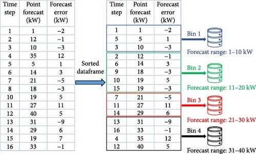
In the following, let t0 denote the current time at which a new prediction is calculated. The algorithmic process steps of the framework are divided into three stages: the deterministic stage, training stage, and forecasting stage, as presented via the process flowchart in Figure 2. For each forecasting period t1, …, tN, all three phases are executed. It is pre-requisite to have sufficient historical deterministic forecasts and measured data y(ti), i < 0 to generate probabilistic predictions.
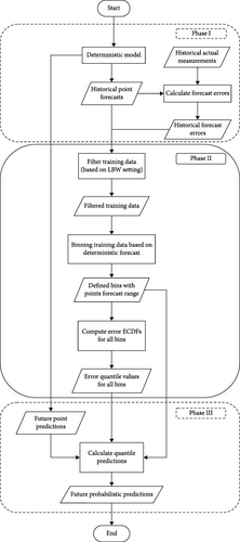
2.1.1. Phase I: Deterministic Stage
In the first phase, a deterministic model is implemented to generate the point forecasts , where N denotes the number of predicted time steps. The UBM is compatible with any deterministic model, be it statistical or machine learning-based. In this study, the statistical method known as the personalized standard load profile (PSLP) is implemented to generate point forecasts for electricity and heat demands, as well as PV generation. Detailed explanations and applications of the PSLP for load forecasting can be found in [39–41]. Additionally, this work integrates and builds upon a recent study [42] that extended PSLP for heat demand and PV generation forecasting. The PSLP is expected to perform poorly for PV forecasting; however, it serves as an example to demonstrate the UBMs performance when a poor performance of the point forecast model is observed.
The historical measured data are collected to train the PSLP model. These data are categorized according to daytype (weekdays, Saturday, and Sunday) and season classifications (summer, transition, and winter), similar to SLPs derived by the German Association of Energy and Water Industries (BDEW) [39]. The daytype classification is not used for PV generation forecasts as it has a very low correlation. Forecasts are then generated by aggregating historical values within each category using statistical measures such as the mean, median, and maximum.
The PSLP training data grows as the model iterates to make it more adaptable to changes in the load profile. That means that the next day incorporates the measured values from the preceding day, and so on. Additionally, a rolling forecast was implemented to limit the training window with the maximum historical days from the day of the forecast, as discussed in [41, 42]. That means the training window slides as it iterates over time, while continuously updating the training data to include recent measurements while excluding older ones beyond the specified window. This approach ensures that the training window does not exceed a specified maximum historical period from the forecast date.
2.1.2. Phase II: Training Stage
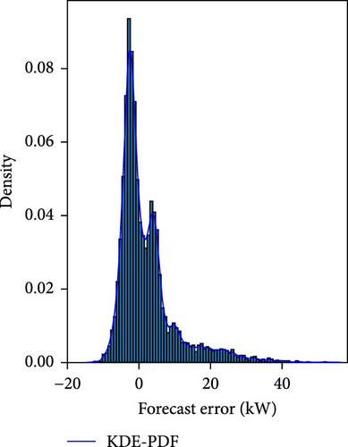
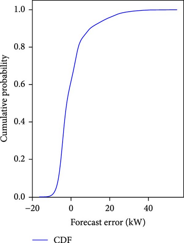
The bandwidth hk in Equation (4) is determined via Scott’s rule [44] , where d = 1 denotes the dimensionality of the data.
Figure 3a shows histogram distribution of the errors and fitting of PDF using KDE, and Figure 3b shows the ECDF of the errors. The point forecast errors at predefined quantiles from the distribution are extracted from the ECDF. In this study, the ECDFs for each bin are obtained using the nearest rank method (NRM), a nonparametric approach. To determine the value of a given percentile q, it selects the corresponding value from the sorted data, such that a proportion q of the data points is smaller than the selected value. A detailed explanation of NRM for this study is given in the following:
Let ej, j = 1, …, nk denote the ordered error values for the kth bin, that is, ej = e(tj), j = 1, …, nk with such that .
The error values at each percentile q for all the bins Bk given by Equation (6) are later used in the forecasting stage to convert point predictions into distributions of forecasts.
The UBM training time series keeps growing as the model iterates over the forecasting time period t1, …, tN to simulate the real case scenario. For example, at the current time t0 and the forecast horizon of 24 h, with the time resolution of 15 min, the measurement and point forecast values for the forecasting period (t1, …, t96) are included in the training set to generate probabilistic predictions for the next forecasting period (t97, …, t192). This means that the UBM is trained after every forecasting period with the new measurements and point forecasts added as part of the training set. This approach enables the capture of any uncertainties in future predictions and adapts to changing conditions. Additionally, in order to prevent an infinite growth of the training data set, the lookback window (LBW) feature is implemented and can be used to set a fixed predefined training window. This should be used as per the requirement and type of data profile to be forecasted. Activating the LBW feature provides the possibility of limiting the training window (with sliding) as the model iterates over the forecasting period t1, …, tN, thus capturing the seasonal trends more accurately and avoid considering old data which are no longer relevant. This feature is implemented in this work to evaluate its potential impact on the performance of the UBM model on all three data profiles. The training windows of 180, 150, 120, 90, and 60 days are considered for analysis. For instance, if the LBW of 180 days is chosen, then the training set for a current time t = 0 will contain the historical point forecast values for i = −1, …, −(180 · m) where m represents the number of data points per day.
2.1.3. Phase III: Forecasting Stage
In this final phase, probabilistic predictions are generated using the trained UBM model. First, a forecasting time period is selected on the basis of the forecast horizon. In this work, the forecast horizon of 24 h was chosen, with the time resolution of 15 min. For instance, at the current time t0, the first forecasting time period spans t1, …, t96. During this period, new point forecasts for i = 1, …, 96 are obtained from the deterministic model. These forecasts are compared with the point forecast intervals (Ik) of all bins Bk as determined in Phase II to identify the appropriate bin at each timestamp.
The process described above is then repeated for each timestamp within the forecasting period to generate a probabilistic prediction curve.
2.2. Performance Evaluation
2.2.1. Deterministic Forecast Evaluation
For PV forecasting, the MAPE metric encounters limitations due to the prevalence of zero measured data. This leads the MAPE calculation in Equation (11) to be undefined. To tackle this problem, the MASE is also implemented, which essentially compares the accuracy of the model with the naive forecast approach. In the MASE calculations for heat forecasts, a naive forecast obtained from the previous week, that is, 7 days ago, is used, whereas for electricity and PV forecasts, the naive forecast from the previous day is used.
2.2.2. Probabilistic Forecast Evaluation
Three main aspects are considered, namely “reliability” or “calibration,” “sharpness,” and “resolution” while evaluating the performance of the probabilistic forecasting [21, 38]. Reliability measures the credibility of the probabilistic forecast model in capturing the actual values within the PI. Sharpness measures the spread of interval width or concentration of predictive distribution. Resolution evaluates the model’s effectiveness in minimizing sharpness while maintaining reliability within an acceptable range. These aspects are assessed using six metrics in this study for a comprehensive evaluation of probabilistic forecasting. All the numerical evaluation metrics are summarized in Table 1.
| Score | PICP | MPIW | WS | QCS | PQCS |
|---|---|---|---|---|---|
| Definition and purpose | Measures the reliability by calculating the percentage of actual values falling within the prediction interval | Measures the sharpness of the prediction interval |
|
Numerical score for GCM, which measures reliability at each quantile bin | Numerical score for GCM, which measures reliability at each quantile bin and overcomes the limitation of QCS, i.e., data size-dependent |
| Unit | Percentage (%) | Unit of entity | None | None | Percentage (%) |
| Interpretation | Higher values indicate better reliability | Lower values indicate better sharpness | Lower scores indicate better overall forecast quality | Lower values indicate better consistency | Lower values indicate better consistency |
| Limitations | Scale-dependent, do not consider reliability at each quantile bin, overestimation of reliability is not penalized | Scale-dependent |
|
Limited when comparing datasets of different sizes, Produces invalid scores during uniform data periods (e.g., zero power generation) | Produces invalid scores during uniform data periods (e.g., zero power generation) |
| Strengths | Good and popular score for measuring overall reliability | Good and popular score for measuring overall sharpness | Takes both reliability and sharpness while scoring | Provides numerical scoring to the visualization GCM score, considers reliability at each quantile bin, not biased toward sharpness over reliability | Overcomes the limitation of QCS being data size-dependent, considers reliability at each quantile bin, not biased toward sharpness over reliability |
- Abbreviations: GCM, graphical calibration measure; MPIW, mean prediction interval width; PICP, prediction interval coverage probability; PQCS, percentage quantile calibration score; QCS, quantile calibration score; WS, Winkler score.
- a.
PICP: The PICP measures reliability within the PI, represented in percentage (%). For a good forecast, PICP is expected to be closely aligned with the PI [35, 49]. PICP is expressed as Equation (13):
- b.
MPIW: The MPIW measures the sharpness of the probabilistic forecasts. However, it is scale-dependent; that is, MPIW is not favorable for comparing probabilistic forecast results for different datasets. A higher PICP and a lower MPIW are desirable, but both conflict with each other [36]. A tradeoff between the PICP and MPIW must be made while evaluating probabilistic forecasts. The MPIW is expressed as Equation (14):
- ()
- c.
WS: The WS considers both reliability and sharpness for evaluation [8]. A low score indicates better probabilistic forecasting. For a central (1 − α) PI, where α ∈ (0, 1), WS is expressed as Equation (15):
- d.
QCS: The QCS assesses reliability with consideration to each quantile bin and penalizes any deviation from expected reliability. In this study, the quantile bins are formed with equal width (10%) percentile ranges (i.e., 0%–10%, 11%–20%,…, 91%–100%). A low QCS value is desired, and the perfect forecast is obtained when the QCS is 0, that is, when the reliability at each quantile bin matches exactly the expected reliability. There is no upper limit for the QCS. It basically rewards when the frequency of observed values (Oi) matches the expected frequency (Ei) at each quantile bin (i) and penalizes deviation from expected frequency (Ei), that is, when high or low sharpness forecasts are obtained for example [32]. The QCS is independent of scale; however, it faces limitations when comparing datasets of different sizes. Additionally, the score becomes invalid for applications with prolonged data uniformity, such as zero power generation in PV forecasting. In such scenarios, all quantile forecasts may converge to the same value (e.g., zero), causing every point to be valid across all quantile bins. This results in significantly inflated Oi for each bin, leading to a disproportionately high QCS due to the penalization for deviations from Ei.
- e.
PQCS: To overcome the limitation of the QCS, the PQCS is implemented, which is expressed as a percentage (%). It is scale- and size-independent; however, like QCS, it becomes invalid for applications with prolonged data uniformity. Lower PQCS values are preferred, with the optimal score being 0%. The PQCS is calculated as Equation (17).
- ()
- f.
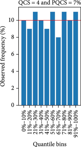
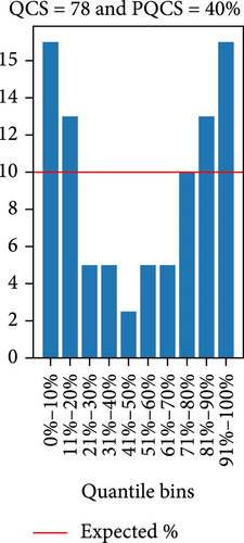
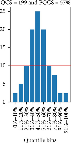
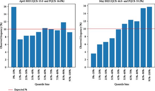
GCM: The GCM is a graphical evaluation tool to assess reliability and sharpness [32]. The GCM plots the bar charts for the actual percentage of observed values (blue-colored bars) in each quantile bin, comparing them to the expected percentage (red line), as shown in Figure 4. Any deviation of actual observed values from the expected observed values for each quantile bin is penalized, resulting in a higher score for its numerical metrics (QCS and PQCS), effectively addressing both under- and overestimations in forecast reliability. Furthermore, the shape of the GCM plot provides insight into the forecast’s sharpness. The perfectly calibrated probabilistic forecasting is obtained when the GCM exhibits a uniform distribution shape, that is, when QCS is 0 and PQCS is 0%. Conversely, the GCM with a triangular shape distribution, as shown in Figure 4c, indicates low sharpness and U-shaped distributions, just as Figure 4b, indicate high sharpness probabilistic predictions, and Figure 4a shows a nearly uniform shaped distribution with low QCS and PQCS values. Both high and low-sharpness forecasts are penalized by the QCS and PQCS because high-sharpness is often unreliable across quantile bins, and low-sharpness probabilistic forecasts are not ideal for decision-making [32]. Figure 4 shows how the QCS and PQCS scores change with the shape of the GCM, offering distinct scores for each of these cases. Moreover, they are not biased toward sharpness over reliability.
3. Case Study
The commercial logistics facility located in northern Germany is considered for the demonstration of the proposed method. This logistics center represents the integration (or “sector–coupling”) of electricity, heat, cooling, and transport. A detailed description of the integrated energy system at the logistics facility can be found in [51]. To verify the effectiveness and accuracy of the method proposed in this paper, the measurements from the ElogZ [52] project are utilized. Electricity and heat meters were installed in different subdistributions of the logistics facility. For this case study, the electricity and heat demand of each subsystem were aggregated. Space heating and the demand for domestic hot water are categorized under the heat sector. To meet these demands, the system utilizes two cascades of air heat pumps, a heat-water buffering storage unit, and two gas boilers to handle peak demand. The cooling needs for the building are met using heat pumps/chillers and a cold water storage unit. The cooling demand is considered in the context of the heating demand for this study. Additionally, servers are equipped with individual air conditioning systems. All electricity needs for the logistics center are supplied by the low-voltage grid. This includes the electricity requirements of the office building, warehouses, dormitories, and other facilities within the center, as well as the energy needs for refrigerated trailers (conditioning, precooling, and maintaining of cold chains) associated with the transport sector. Figure 5a,b depicts the office building (business center) and dormitory, respectively. Recently, rooftop PV panels were installed in the warehouse to boost local electricity generation for the facility, as shown in Figure 5c. Due to the lack of PV generation measurement data for this study, PV generation was simulated with a system size of 200 using the Python library pvlib [53], utilizing publicly available weather data obtained from open DWD [54]. The assumption made in the simulation for the PV modules is that they are oriented half to the east and half to the west, with an inclination angle of 10°. Battery and power electronics for control are installed in the dormitory, as depicted in Figure 5d. Air source heat pump systems are also integrated within this facility. Both deterministic and probabilistic forecasts are generated as an essential component of the EMS for the given distributed integrated energy system. The observation, forecasting, and waiting periods for both methods are detailed in Table 2. All of the data used in this study, including measured values and generated point and probabilistic forecasted output results, were considered at a 15-min resolution and represented in kW. The forecasting framework (UBM) and its evaluation are implemented in Python programing language.



| Forecasting parameters | Deterministic forecast (PSLP) | Probabilistic forecast (UBM) |
|---|---|---|
| Observation period | 5 Sep 2021–30 Aug 2022 | 26 Sep 2021–30 Aug 2022 |
| NWDs | 21 days | 7 days |
| Forecasting period | 26 Sep 2021–30 Aug 2022 | 5 Oct 2021–30 Aug 2022 |
- Abbreviations: NWDs, number of waiting days; PSLP, personalized standard load profile; UBM, uncertainty binning method.
4. Results
4.1. Deterministic Forecast
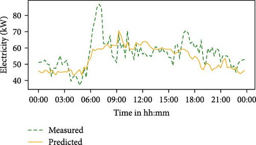
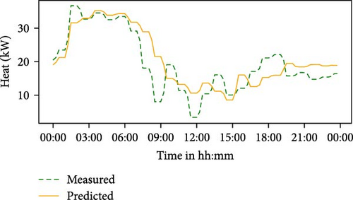
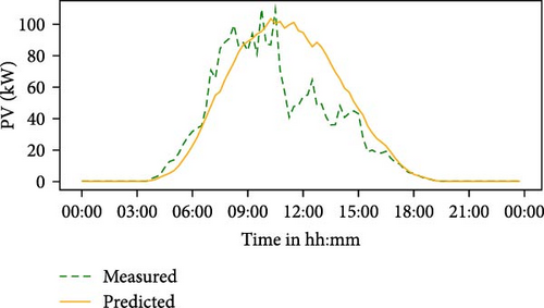
In this section, the forecast results and accuracy of the PSLP for electricity, heat, and PV profiles are presented and compared. After setting the number of waiting days (NWDs) to 21 as the basis for the PSLP, point forecasts were generated for a period between 26 September 2021 and the end of August 2022, as shown in Table 2. For the same period, the mean of the evaluation scores for the electricity demand, heat demand, and PV generation were obtained, as displayed in Table 3. Figure 6 illustrates the PSLP forecasts and its comparison with the actual values for a random day (8 June 2022). The mean MAE for the electricity (6.34 kW) and heat demand forecasts (6.4 kW) are within a similar range, whereas the PV generation forecasts exhibit a higher value of 9.9 kW.
| Sector | Scores | ||||
|---|---|---|---|---|---|
| MAE (kW) | MSE (kW) | RMSE (kW) | MAPE (%) | MASE | |
| Electricity | 6.34 | 78.29 | 8.71 | 13.18 | 0.65 |
| Heat | 6.4 | 76.65 | 8.52 | 26.55 | 0.6 |
| PV | 9.9 | 441.76 | 20.62 | — | 0.93 |
- Abbreviations: MAE, mean absolute error; MAPE, mean absolute percentage error; MASE, mean absolute scaled error; MSE, mean square error; PSLP, personalized standard load profile; RMSE, root mean square error.
Moreover, a high MSE value of 441.76 kW for the PV forecasts indicates that there are significant forecast errors on numerous timestamps throughout the forecasting period. The lowest MAPE score was obtained for electricity (13.18%), followed by the heat (26.55%). With respect to MASE, it can be observed that the PSLP performed better than the naive forecast for all of the sectors, as it was below 1.
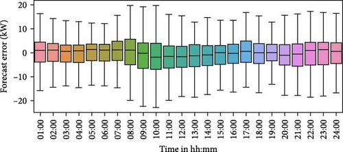
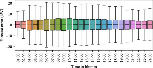
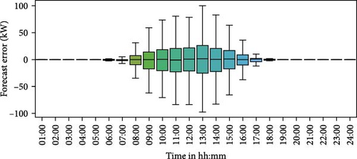
The hourly forecasting error distribution for the entire forecasting period in a boxplot format is shown in Figure 7. The box represents the interquartile range (IQR), which encompasses the values between the 25th and 75th percentiles. The black line inside the box represents the median, which corresponds to the 50th percentile (the median). The upper and lower whiskers extend from the box by a maximum of 1.5 times the IQR. Figure 7 illustrates that the PV predictions exhibit wider error spread distributions during the daytime hours compared to heat and electricity demand forecasts. That means the PSLP resulted in poor forecasting for PV generation, as expected, which could impact decision-making in EMS. In such cases, probabilistic forecasting using UBM could be beneficial for informed decision-making, as elaborated upon in Section 5.
4.2. Probabilistic Forecast
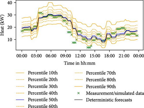
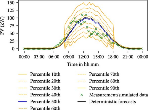
In this section, the forecast results and accuracy of the UBM for the electricity, heat, and PV profiles are presented. In this study, the NWD for the UBM was 7 days, resulting in the generation of probabilistic forecasts from 3 October 2021 to the end of August 2022, as shown in Table 2. The probabilistic forecasts compromise percentiles ranging from 10% to 90%, representing an 80% PI and forming the basis for its performance evaluation. Later, the forecasts were also evaluated with different PI levels of 40% and 60%. Several forecast evaluation metrics (PICP, MPIW, GCM, QCS, and PQCS) are used to assess its performance, as discussed in Section 2.2.2. The PICP and MPIW were calculated daily, while the QCS and PQCS were computed monthly to ensure an adequate number of data points for their calculation. The QCS and PQCS metrics are not applicable to PV, as the predictions at different percentiles often coincide with the measured values, particularly during periods of zero power generation, as exemplified in Figure 8.

4.3. Probabilistic Forecast Results Without LBW Feature
The mean of the evaluation metrics presented in Table 4 were computed for the probabilistic forecasting period (Table 2), with the LBW feature being inactive. This means that the training dataset progressively expands over the forecasting period without being limited by the training window. Monthly PICP, MPIW, WS, QCS, and PQCS were averaged over the entire forecasting period across sectors for different number of bins, as shown in Table 4. Figure 8 shows the probabilistic output results from the UBM for a random day (8 June 2022). On this day, it was observed that the UBM performed with high reliability across all sectors; that is, the majority of the measured values, denoted by green crosses, fall within the PI. However, the UBM exhibited low-sharpness PV forecasts, especially during peak generation hours.
| Sector | Number of bins | Scores | ||||
|---|---|---|---|---|---|---|
| PICP (%) | MPIW (kW) | WS | QCS | PQCS (%) | ||
| Electricity | 3 | 80.32 | 19.71 | 30.81 | 21.23 | 21.13 |
| 7 | 79.52 | 19.59 | 30.54 | 20.99 | 20.95 | |
| 9 | 78.95 | 19.48 | 30.57 | 23.63 | 22.48 | |
| 12 | 79.04 | 19.52 | 30.66 | 22.62 | 21.88 | |
| Heat | 3 | 82.32 | 22.42 | 31.64 | 27.43 | 23.95 |
| 7 | 81.45 | 22.29 | 31.59 | 23.31 | 22.53 | |
| 9 | 81.55 | 22.33 | 31.54 | 29.88 | 25.25 | |
| 12 | 80.89 | 22.05 | 31.88 | 30.03 | 25.72 | |
| PV | 3 | 81.32 | 26.06 | 59.30 | — | — |
| 7 | 80.62 | 30.09 | 50.99 | — | — | |
| 9 | 80.46 | 31.40 | 49.45 | — | — | |
| 12 | 81.37 | 32.54 | 48.58 | — | — | |
- Abbreviations: MPIW, mean prediction interval width; PICP, prediction interval coverage probability; PQCS, percentage quantile calibration score; QCS, quantile calibration score; UBM, uncertainty binning method; WS, Winkler score.
From Table 4, the analysis reveals that the UBM model consistently generated reliable probabilistic forecasts with different number of bins across all sectors, with the average PICP being closely aligned with the PI level (80%). For the electricity forecast, the highest PICP (80.32%) was obtained with three bins, but at the same time highest MPIW (19.71 kW), that is, the lowest sharpness, was observed. Considering the WS, QCS, and PQCS, the best forecast for electricity was obtained with seven bins. For the same, the WS, QCS, and PQCS are 30.54%, 20.99%, and 20.95%, respectively. For the heat demand forecast, the highest PICP was obtained with three bins; however, this also resulted in the lowest sharpness, that is, the highest MPIW of 22.42 kW. While the lowest WS (31.54) was observed with nine bins. Considering QCS and PQCS, the best forecast for the heat sector was obtained with seven bins, yielding QCS and PQCS values of 23.31% and 22.53%, respectively. For the PV forecast, the best UBM accuracy was achieved with 12 bins, which corresponded to the lowest WS of 48.58. However, it is worth noting that this also resulted in the lowest sharpness, as indicated by the highest MPIW among the bin configurations. Based on the overall scores in Table 4, the optimal number of bins for electricity, heat, and PV were determined to be 7, 7, and 12, respectively. Consequently, the results presented are derived from this selection of the number of bins for each sector. Figure 9 illustrates the comparison of scores across different sectors based on their respective optimal bin configurations.
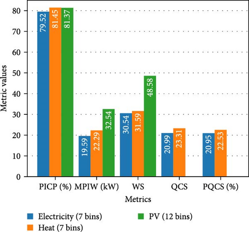
From Figure 9, it can be observed that UBM achieved the highest PICP value of 81.45% for heat forecasts, whereas the lowest PICP value was obtained for electricity forecasts. With respect to the MPIW, the UBM excels in producing sharp forecasts for electricity (19.59 kW) and heat demand (22.29 kW) compared to PV generation (32.54 kW). A high interval width (i.e., low sharpness) was observed for PV generation, which can be interpreted from a high MPIW. Conversely, the UBM achieved the highest sharpness (i.e., lowest MPIW) for the electricity profile with a value of 19.59 kW. The lowest WS was observed for electricity (30.54), followed by heat (31.59), but exhibited notably high WS for PV (48.58). Considering the variability of PV generation and inaccuracy of the PSLP forecasts output, a high MPIW and WS were observed, as expected. Based on the QCS and PQCS, the highest calibrated forecast was observed for electricity, with values of 20.99 and 20.95%, respectively, compared to the heat sector, with values of 23.31% and 22.53%, respectively.
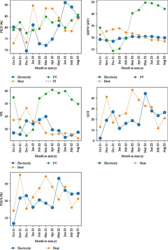
The performance of the UBM, as measured by PICP, MPIW, WS, QCS, and PQCS, on the electricity, heat, and PV data profiles for each month throughout the forecasting period, is depicted in Figure 10, with the LBW feature being inactive. The black dashed line in the first subplot depicts PI (i.e., 80%) to indicate the deviation from the expected PICP. Notably, higher PICP values were observed in the spring and summer months compared to the winter months. During the same period, higher MPIW values for PV were observed, possibly due to higher fluctuation in the data profile. The MPIW for the electricity experienced a slight rise during the spring and summer, while the opposite trend was observed for a heat profile. The trend of the WS can be interpreted by combining the trends of the PICP and MPIW. The lowest WS for PV (24.79 kW) was observed in December 2021, while the lowest WS for electricity (23.62 kW) and heat (22.83 kW) was observed in June 2022 and August 2022, respectively. Moreover, the monthly QCS and PQCS values were observed for the electricity and heat profiles. The lowest QCS and PQCS values for electricity (2.2% and 6.8%, respectively) were observed in October 2021. The lowest QCS and PQCS values for the heat forecasts were 11.8 in July 2022 and 14.2% in October 2021, respectively. The highest QCS and PQCS, that is, the lowest reliability at each bin for the electricity profiles, were observed in May 2022 with values of 44% and 33.2%. On the other hand, for the heat profile, the highest QCS (47.5) and PQCS (35.1%) were observed in March 2022 and November 2021, respectively. Overall, the UBM demonstrated relatively good accuracy for electricity compared to the heat sector based on WS, QCS, and PQCS. The GCM plots for the electricity in April and May 2022 are shown in Figure 11 as an example. It was observed that both the QCS and PQCS penalize deviations from the expected percentage. This is evident in the way the values of QCS and PQCS change with the shape of the GCM, making them valuable scores for further investigating the accuracy of the probabilistic forecasts. They offer a more comprehensive reliability assessment, along with insights into the sharpness of probabilistic forecasting.
The results presented above were based on 80% PI as a benchmark for evaluating the probabilistic forecast. In the following, forecasts are evaluated across different PI levels, including 40% and 60%, using the optimal bins for each sector, as given in Table 5. A PI of 100% is excluded from consideration because it encompasses all possible outcomes, making it overly broad and uninformative for practical decision-making in energy management. It fails to provide actionable insights or the precision needed to assess risks or optimize resource allocation, which is essential for the intended application. The QCS and PQCS remain unchanged across different PI levels, as they are computed considering the entire quantile range from 0% to 100% with a fixed bin width of 0.1th or 10th percentile. Consequently, these metrics are not included in Table 5. It can be observed that the PICP remains closely aligned with the PI levels for each sector, except for the PV with a 40% and 60% PI, which resembles over-coverage, reflected in a PICP value of 67.33% and 74.41%, respectively. From Table 5, it is evident that with increased PI levels, the interval width also increases, as indicated by MPIW values, to cover the expected real values within the quantile range. This leads to also increase in WS, as the score emphasizes sharpness, as discussed in Section 2.2.2.
| Sector | Scores | |||
|---|---|---|---|---|
| PI (%) | PICP (%) | MPIW (kW) | WS | |
| Electricity | 40 | 39.7 | 7.55 | 18.76 |
| 60 | 59.28 | 12.36 | 23.13 | |
| 80 | 79.52 | 19.59 | 30.54 | |
| Heat | 40 | 42.99 | 8.3 | 19.34 |
| 60 | 63.22 | 13.9 | 24.01 | |
| 80 | 81.45 | 22.29 | 31.59 | |
| PV | 40 | 67.33 | 13.96 | 29.67 |
| 60 | 74.41 | 22.07 | 36.53 | |
| 80 | 81.37 | 32.54 | 48.58 | |
- Abbreviations: MPIW, mean prediction interval width; PI, prediction interval; PICP, prediction interval coverage probability; UBM, uncertainty binning method; WS, Winkler score.
4.4. Probabilistic Forecast Result With LBW Feature
To show the effect of the LBW feature on the UBM performance, evaluation metrics were calculated for electricity, heat, and PV with varying sliding training windows (180, 150, 120, 90, and 60 days) with an optimal number of bins and PI of 80%, as shown in Table 6. For all the data profiles, reducing the training window led to a slight decrease in the MPIW, WS, QCS, and PQCS. However, it should be noted that PICP also decreases simultaneously. The decrease in these metrics can be attributed to the smaller training dataset size, leading to lower data variability over shorter time frames. Consequently, this results in a reduced spread of error distributions, subsequently lowering evaluation metrics values. In the case of electricity, the lowest MPIW (19.67 kW), QCS (18.25), and PQCS (18.71%) were obtained with a training window of 60 days. However, the PICP was lowest (78.13%) compared to the other training windows. On the other hand, the lowest WS (30.54) was obtained with a training window of 90 days. The choice between achieving a higher reliability or a higher sharpness depends on the specific application. In the case of the heat profile, the lowest WS (31.02) was obtained with a 90-day training window, whereas the lowest QCS (18.96) and PQCS (19.97) scores were obtained with 60 days. For the PV forecasts, the highest PICP and lowest WS was achieved with a 150-day training window. However, overall, it can be said that with shorter training window results in better performance of probabilistic forecasting, considering WS, QCS, and PQCS, which take both reliability and sharpness into account.
Training horizon |
Scores | ||||
|---|---|---|---|---|---|
| PICP (%) | MPIW (kW) | WS | QCS | PQCS (%) | |
| Electricity | |||||
| 180 days | 79.65 | 19.75 | 30.66 | 21.16 | 21.12 |
| 150 days | 79.77 | 19.81 | 30.61 | 20.15 | 20.63 |
| 120 days | 79.55 | 19.8 | 30.6 | 18.33 | 19.39 |
| 90 days | 79.17 | 19.8 | 30.54 | 17.88 | 18.91 |
| 60 days | 78.13 | 19.67 | 30.6 | 18.25 | 18.71 |
| Heat | |||||
| 180 days | 80.0 | 21.46 | 31.33 | 25.55 | 23.16 |
| 150 days | 79.67 | 21.2 | 31.27 | 23.95 | 22.78 |
| 120 days | 78.95 | 20.81 | 31.11 | 21.55 | 21.12 |
| 90 days | 78.37 | 20.6 | 31.02 | 22.67 | 21.45 |
| 60 days | 78.3 | 20.58 | 31.09 | 18.96 | 19.97 |
| PV | |||||
| 180 days | 81.32 | 31.36 | 48.85 | — | — |
| 150 days | 81.32 | 31.33 | 47.98 | — | — |
| 120 days | 81.23 | 30.74 | 48.69 | — | — |
| 90 days | 81.37 | 30.25 | 48.37 | — | — |
| 60 days | 81.11 | 29.6 | 48.52 | — | — |
- Abbreviations: LBW, look back window; MPIW, mean prediction interval width; PICP, prediction interval coverage probability; PQCS, percentage quantile calibration score; QCS, quantile calibration score; UBM, uncertainty binning method; WS, Winkler score.
5. Discussions
Due to the increased uncertainty and requirement of low-cost EMS at the distribution level, a simple and robust forecasting framework (UBM) was introduced in this study. It was found to be computationally fast, reliable, adaptable across sectors, low feature engineering, and relies on easily accessible data. The UBM generates probabilistic forecasting by levering deterministic models, in this case, PSLP. The electricity demand, heat demand, and PV generation forecasting were produced for the distributed integrated energy system at a logistics facility in northern Germany. This work also emphasizes the limitations of commonly used evaluation metrics for probabilistic forecasting and illustrates how a more comprehensive evaluation can be achieved by incorporating new metrics such as GCM, QCS, and PQCS.
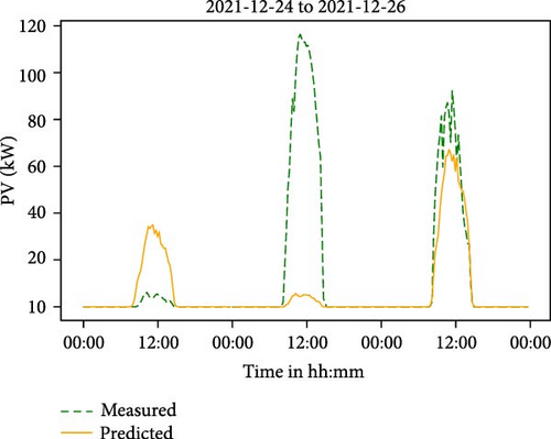
The PSLP was evaluated using popular metrics (MAE, MSE, RMSE, MAPE, and MASE) for all the sectors. The mean of these metrics across the entire forecasting period was calculated, and it was found that the PSLP performed better for electricity and heat demand forecasts but exhibited high forecasting errors for PV generation, as expected. This shortcoming can be attributed to the inherent variability in PV generation, as illustrated in Figure 12, where generation over three consecutive days highlights the significant variability and notable forecast errors incurred by the PSLP model. This will directly affect probabilistic forecasting generated by the UBM.
The UBM performance was evaluated with a different number of bins for each sector. The optimal bins for electricity, heat, and PV were found to be 7, 7, and 12 bins. The UBM demonstrated highly reliable probabilistic forecasting across sectors. However, it fails to provide a sharp PV generation forecast. Notably, low sharp probabilistic forecasts were observed mostly during the PV peak hours. This is mainly due to the high variability of PV generation itself, which consequently leads to high forecast errors generated by the PSLP model. This, in turn, results in a wider spread of point forecast errors during the peak PV generation hours, as depicted in Figure 7c. This corresponds to the wider error ECDFs for the clusters in Phase II of the UBM model. Consequently, this leads to wider interval widths (i.e., low sharpness) in the generated probabilistic forecast in Phase III, as shown, for example, in Figure 8c.
Low sharpness in probabilistic forecasting can pose challenges for effective decision-making when compared to real behavior. Decision-makers rely on forecasts not only to assess reliability but also to ensure the intervals are sufficiently narrow to facilitate actionable insights. Forecasts with low sharpness imply broad uncertainty bands, which may be interpreted as a lack of confidence in the forecast’s precision. In practical terms, this can lead to overly conservative decisions, such as over-provisioning resources or failing to optimize the deployment of assets like energy storage systems. For instance, in energy management, a forecast with wide PIs might hinder effective grid balancing or delay response strategies, thus impacting the cost-effectiveness and efficiency of operations. Nevertheless, even when a deterministic model demonstrates significant forecasting errors, as in the case of PV, probabilistic forecasting emerges as highly valuable from a decision-making perspective. It provides critical insights into the degree of uncertainty associated with the model’s forecasted outputs. Depending solely on inadequate point forecasts can pose substantial challenges across a multitude of applications within a power system. Therefore, the UBM is found to be a highly valuable tool, capable of converting inaccurate point forecasts into reliable probabilistic ones and providing richer information about uncertainty for decision-making in energy management.
In future work, the implementation of more accurate point forecast models for PV generation could be explored to achieve more precise probabilistic forecasting results from the UBM, however, this is out of scope for this work. Since the UBM’s performance relies heavily on the accuracy of the underlying deterministic model, any limitations or inaccuracies in the point forecast can directly impact the quality of the probabilistic forecast. Therefore, improving the base deterministic model for PV generation is essential to enhance the sharpness and overall reliability of the UBM’s output. By integrating advanced forecasting models that better capture the high variability and complex patterns of PV generation, such as hybrid machine learning approaches or enhanced statistical models, the UBM could potentially generate tighter PIs and reduce the spread of errors observed during peak generation periods. This would ultimately lead to more actionable and trustworthy forecasts, facilitating more effective decision-making and resource management within power systems.
Overall, a correlation between the accuracy of the deterministic model (PSLP) and the UBM model was also observed. As the point forecasts and its errors are used as training data for the UBM, their impact on the model’s performance becomes evident. A higher variability in the data profile and lower accuracy of the deterministic model results in low sharpness probabilistic predictions. Typically, the UBM compromises sharpness by prioritizing the PICP to be closer to or higher than the PI. In order to obtain a better PICP, the interval width must simultaneously increase. On the other hand, reducing the PI can improve the sharpness, but this does not necessarily enhance the overall accuracy of the probabilistic forecasts. But, the UBM at all time tries to achieve reliable forecasts, even if sharpness is compromised. This investigation sheds light on how the performance of the deterministic model influences the sharpness and reliability of the probabilistic forecasts produced by the UBM. Ultimately, this insight supports informed decision-making in EMS.
UBM was also evaluated with different PI levels. PICP values were found to be aligned with PI levels being considered for all the sectors, except for PV, with PI of 40% and 60%. It is usually expected to have a PICP closer to PI; therefore, overestimating the PICP beyond the expected PI level indicates that the model is overestimating the level of uncertainty or variability in the PV generation, leading to wider intervals that cover more of the actual data points than anticipated. This over-coverage can be problematic in energy management because it may lead to inefficient decision-making, such as overestimating the reserve capacity needed or over-allocating resources to account for higher-than-expected variability. With the increase in PI levels, the interval width also increased as expected, ensuring that the forecasted intervals covered the real values within the quantile range.
Moreover, the UBM implemented the LBW feature, which basically limits and slides the training window as the model iterates over the time. It was observed that reducing the training window decreases sharpness (MPIW and WS) but has a slight effect on reliability (PICP). Overall, it was observed that with shorter training window results in better performance of the UBM. Across all given data profiles, the effect of changing the training window on the performance of the UBM was not significant. However, even a slight improvement in forecasting results counts. Slightly higher differences were observed in electricity and heat demand forecasts based on the QCS and PQCS. Although the effect on the data profiles in this study was not substantial, it could be more significant for other data profiles. Therefore, testing the LBW feature to assess its impact on the UBM, depending on the data profile, can be useful for improving the accuracy of the UBM. As a guideline for selecting an appropriate training window, observations from this study suggest the following: for data profiles with pronounced seasonal variations, such as PV generation and heat demand, a training window of 30–90 days is recommended. This range ensures that the training data reflects season-specific characteristics, as using historical data from a season like summer to construct forecast distributions for winter could lead to reduced sharpness. Conversely, electricity demand profiles may accommodate a larger training window (e.g., over 90 days), but this depends on the nature of the connected load. In the future, as the number of heat pumps increases, winter demand is expected to grow relative to summer, amplifying seasonal differences. In such scenarios, a shorter training window (e.g., 30–90 days) would again be advisable. However, it is important to note that shorter training windows result in fewer data points within each cluster, potentially hindering the generation of accurate error distributions. Overall, the selection of the training window should be tailored to the specific characteristics of the case at hand.
Table 7 compares UBM with several known models or approaches that leverage the deterministic model to generate probabilistic forecasts. The GCM, QCS, and PQCS overcome some of the shortcomings of popular metrics. The GCM offers a graphical evaluation, which is not commonly found in the literature on probabilistic forecasting evaluation. PIT is a similar technique as GCM that has been described in other literature [30, 31], but it lacks numerical representation, which is addressed by QCS and PQCS in this study. The QCS and PQCS are independent of the data scale, in contrast to MPIW and WS. This supports the comparison of model’s performance based on different datasets. Furthermore, QCS and PQCS are not biased toward sharpness over reliability, as in the case with WS. Unlike PICP, which only measures the reliability within the PI, QCS, and PQCS assess reliability with consideration to each quantile bin and check its deviation from expected reliability. That is, they penalize any over and underestimation of reliability. However, these metrics cannot be applied to PV, as the predictions at various percentiles align with the measured values, particularly during periods of zero power generation, leading to significantly inflated observed frequency (Oi) for each bin. This results in disproportionately high QCS and PQCS due to the penalization for deviations from expected frequency (Ei). An alternative approach could involve excluding such occurrences when calculating QCS and PQCS, enabling their use in evaluating probabilistic forecasting of PV generation. In future work, the adaptation of QCS and PQCS for PV generation should be prioritized to provide a fair evaluation framework. Developing modified versions of these metrics or applying conditional calculations would enhance their applicability. This would support more nuanced insights into forecasting performance and better guide decision-making. There is no single metric that can evaluate all aspects of probabilistic forecasting without limitations. Therefore, in addition to popular metrics (PICP, MPIW, and WS), GCM and its numerical scores (QCS and PQCS) can provide a more comprehensive and intuitive performance assessment.
| Method | Limitations | Strengths | Sources |
|---|---|---|---|
| QRA |
|
|
[14–16] |
| QRF |
|
|
[3, 22, 23] |
| EPIs |
|
|
[26–28] |
| AnEn |
|
|
[33, 34] |
| UBM |
|
|
This study |
- Abbreviations: AnEn, analog ensemble; EPIs, empirical prediction intervals; QR, quantile regression; QRA, quantile regression averaging; QRF, quantile random forest; UBM, uncertainty binning method.
There are numerous possibilities for enhancing the accuracy of the UBM, primarily by considering more precise deterministic models, especially in the case of PV forecasting. Besides the deterministic methods, alternative binning approaches can be explored for the UBM training. This work uses the Python “cut” function [55], which requires to predefined the number of clusters and discretizes the data with equal-width bins. An alternative approach is the Python “qcut” function [56], which discretizes arrays into equally sized bins. This enables the function’s algorithm to generate clusters based on the data profile itself while maintaining an equal number of data points in each bin. Such flexibility in generating clusters should be data-driven rather than being preset to predefined clusters. There are other popular automatic clustering algorithms, such as K-means and fuzzy C-means clustering [57–59] that could be implemented to train the UBM. Furthermore, hyperparameter optimization could enhance the UBMs performance further.
6. Conclusions and Outlook
This work introduces an approach to generating probabilistic forecasting by extending a deterministic model. Given the increasing significance of uncertainty quantification in the energy domain, the proposed UBM emerges as a valuable tool for decision-making in EMS. It is shown to be a transparent and efficient method that leverages deterministic models while offering simplicity and high computational speed, harnesses readily available data, requires minimal training data, involves minimal feature engineering, offers rapid computational capabilities, and achieves reasonable accuracy. This approach caters to the evolving landscape of EMS requirements, particularly in smaller-scale settings like buildings and mid-sized facilities, where efficiency and affordability are the main factors. The UBM was rigorously validated for forecasting electricity demand, heat demand, and PV generation. A practical case study was conducted using an existing distributed integrated local energy system at a logistics facility in northern Germany.
The statistical PSLP method was implemented to generate point forecasts, which were subsequently used as input features for the UBM. For its evaluation, MAE, MSE, RMSE, MAPE, and MASE were considered. The PSLP model demonstrated good performance in forecasting the electricity and heat demand but exhibited limitations in accurately predicting PV generation. As UBM uses point forecasts from the PSLP model as input features for generating probabilistic forecasts, the accuracy of the PSLP impacted the UBMs overall accuracy. This impact was particularly noticeable in the interval width, as evident through MPIW and WS. In the given case study, sensitivity analysis was carried out to determine the optimal number of bins on the performance of the UBM, which resulted in the selection of 7, 7, and 12 bins for electricity, heat, and PV, respectively. Following the selection of optimal bins, it was observed that the UBM achieved notably good reliability across all sectors, with PICP values of 79.52%, 81.45%, and 81.37 % for electricity, heat, and PV, respectively. With respect to sharpness, the UBM showed better performance on electricity and heat demand over PV generation. A high MPIW (32.54 kW) and WS (48.58) were observed for PV generation forecasts, which can be attributed to the low accuracy of the PSLP model due to the high variability of the data profile itself. Hence, it was observed that the accuracy of the point forecast model directly impacts that of the probabilistic forecasts produced by the UBM. However, it has the capability to transform inaccurate deterministic forecasts into reliable probabilistic ones, providing richer information on uncertainty and, consequently, supporting decision-making in EMS. To address the limitations of popular evaluation scores, the GCM, QCS, and PQCS were implemented, providing a more comprehensive performance evaluation of probabilistic forecasting. Both the QCS and PQCS scores were found to be better for electricity, with values of 20.99% and 20.95%, respectively, compared to heat, with the QCS value of 23.31 and PQCS value of 22.53 %. However, the scores were found to be unsuitable for evaluating PV forecasts. The UBMs performance was also evaluated at different PI levels (40%, 60%, and 80%). The PICP was found to be closely aligned with PI levels for each sector, except for PV, with 40% and 60% PI. The interval width was found to be increased with an increase in PI levels, as expected, resulting in higher MPIW and WS. Moreover, performance evaluations were conducted with varying sliding training windows. It was observed that the reduction in the training window yielded an improvement in the probabilistic forecast scores except PICP.
Future work should focus on testing the UBM with more accurate deterministic models, especially for PV. Moreover, K-means clustering, fuzzy C-means clustering, qcut, or other more advanced clustering techniques should be explored for training the UBM. A detailed comparison of the UBM with other available probabilistic forecasting techniques should be investigated in further work. The adaptation of the GCM, QCS, and PQCS for PV probabilistic forecasts is another avenue to be considered. Further detailed examination is required on how point forecast errors propagate to the accuracy of the UBM. In the future, the real application of the UBM for operational optimization can be tested, for example, by optimizing EV charging schedules. Although the potential applications of the UBM within the distributed integrated local energy systems are abundant, these possibilities remain avenues for exploration in future research.
Nomenclature
-
- AnEn:
-
- Analog ensemble
-
- BEVs:
-
- Battery electric vehicles
-
- ECDF:
-
- Empirical cumulative distribution function
-
- ELogZ:
-
- Energieversorgungskonzepte für Klimaneutrale Logistikzentren
-
- EMS:
-
- Energy management system
-
- EPI:
-
- Empirical prediction interval
-
- GCM:
-
- Graphical calibration measure
-
- IQR:
-
- Interquartile range
-
- KDE:
-
- Kernel density estimation
-
- LBW:
-
- Look back window
-
- MAE:
-
- Mean absolute error
-
- MAPE:
-
- Mean absolute percentage error
-
- MASE:
-
- Mean absolute square error
-
- MPIW:
-
- Mean prediction interval width
-
- MSE:
-
- Mean square error
-
- NRM:
-
- Nearest rank method
-
- NWDs:
-
- Number of waiting days
-
- PDF:
-
- Probability density function
-
- PI:
-
- Prediction interval
-
- PICP:
-
- Prediction interval coverage probability
-
- PIT:
-
- Probability integral transform
-
- PQCS:
-
- Percentage quantile calibration score
-
- PSLP:
-
- Personalized standard load profile
-
- PV:
-
- Photovoltaic
-
- QCS:
-
- Quantile calibration score
-
- QR:
-
- Quantile regression
-
- QRA:
-
- Quantile regression averaging
-
- QRF:
-
- Quantile random forest
-
- RMSE:
-
- Root mean square error
-
- SLP:
-
- Standard load profile
-
- UBM:
-
- Uncertainty binning method
-
- WS:
-
- Winkler score.
Disclosure
Responsibility for the content of this publication lies with the author. More information regarding the ELogZ can be found at www.elogz.de.
Conflicts of Interest
The authors declare conflicts of interest.
Funding
The project Energieversorgungskonzepte für klimaneutrale Logistikzentren (ELogZ) on which this article is based was funded by the Federal Ministry for Economic Affairs and Climate Action (BMWK) under the funding code 03EN1015F.
Acknowledgments
The authors gratefully acknowledge PANEUROPA Transport GmbH for the provision of time series data, pictures, and knowledge of its logistics facility under the project “Energieversorgungskonzepte für klimaneutrale Logistikzentren (ELogZ).”
Open Research
Data Availability Statement
The authors do not have institutional permission to share data or codes.


