An Approachable Anaerobic Bioreactor for Remote Biogas Production: Experimental Analysis and Neuroevolution Modeling
Abstract
This study introduces a straightforward batch-mode bioreactor for the production of biogas from two waste sources: animal slaughterhouse solid waste and fruit and vegetable solid waste, as well as poultry slaughter solid waste and fruit and vegetable solid waste. To measure the efficiency of methane and carbon dioxide (CO2) production, the system was experimentally studied for 40 days, investigating different carbon-to-nitrogen (C/N) ratios: 20, 30, and 40. The highest biogas and methane contents were observed at a C/N ratio of 30. The poultry slaughterhouse waste (SHW) and fruit and vegetable waste (FVW) combination resulted in an impressive 201.7 L of biogas, with 149.2 L of pure methane. Similarly, the animal SHW and FVW mixture resulted in 241 L of biogas, containing 182.7 L of valuable methane. Recognizing the complex nature of factors that impact the anaerobic digestion (AD) process, this study employed kinetic models and artificial neural networks (ANNs) combined with three optimizers: Differential Evolution (DE), Bacterial Foraging Optimization (BFO), and the Dragonfly Algorithm (DA). The simulation data revealed that the BFO approach yielded the best models. Notably, the mean squared error (MSE) during the testing phase was remarkably low, measuring 0.000552 for cumulated CO2 production and 0.001598 for cumulated methane production. Overall, the models introduced in this study exhibit excellent generalization capability and serve as reliable predictors for the systems’ output in various scenarios. The significance of these findings extends beyond the laboratory, as the proposed system and its model can effectively aid end-users in planning their consumption and correlating biogas utilization with peak production. This mainly benefits small consumers in remote areas, offering them sustainable energy solutions and paving the way for a greener future.
1. Introduction
Anaerobic digestion (AD) is an attractive fermentative process that transforms various types of biodegradable substrates into biogas, usually in the form of waste. The stability of the AD process when using single substrates can be impacted by the accumulation of volatile fatty acids (VFAs) as well as long-chain fatty acids, which interrupts the performance of methanogenic bacteria [1, 2]. Moreover, the process can suffer from incomplete breakdown and pH reduction, which inhibit methanogenesis [3]. Additionally, the pH value of substrates affects the growth of methane-producing microorganisms. It also effectively decomposes some essential compounds in the AD process, resulting in ammonia, sulfide, and organic acids [4]. Investigations indicate methane production occurs in a relatively narrow pH range of 6.5–8.5, with the optimal range for most methanogenic bacteria being 7–8. Therefore, if the pH value decreases below 6 or increases above 8.5, this process is inhibited, and if the pH falls below 5.5, the methanogenic bacteria are inactivated [5].
To overcome this limitation and increase methane production, codigestion of different raw materials can be a viable alternative to using single substrates [6]. Codigestion involves the simultaneous digestion of two or more organic substrates to enhance biogas production. This is achieved by carefully selecting a blend ratio that balances the carbon-to-nitrogen (C/N) ratio, thereby preventing inhibition and ensuring a favorable nutrient and moisture equilibrium [7]. The advantages of this approach include improved biogas production went up by 25%–400%, which results from an increased diversity of microbial communities, reduction of toxic compounds such as heavy metals, reduction of antibiotic-resistant genes and bacteria, and the increase of codigestate bioavailability [8, 9]. Studies in this field have revealed that solid wastes from slaughterhouses, like sludge generated in wastewater treatment plants and livestock and poultry carcasses, contain a considerable quantity of protein, fat, and organic materials that can be effectively converted into biogas [10]. In contrast, vegetable processing waste (VPW) exhibits a high C/N ratio, making it suitable for anaerobic codigestion in concert with slaughterhouse wastes (SHWs).
Despite its numerous benefits, AD is a complex procedure that is not universally compatible with all types of feedstocks. It is also more challenging to manage than single substrate AD because achieving optimal results necessitates meticulous control over feedstock composition and operating conditions. Given the considerable variation in feedstock type and quality, biogas production facilities often encounter a range of challenging decisions in their day-to-day operations. Unfortunately, these decisions are typically based on qualitative assessments rather than rigorous data analysis [9]. Thus, a top-priority requirement exists to develop a systematic approach for modeling, optimizing, predicting, and controlling AD process performance to support decision-making and improve resource utilization and output quality efficiency.
Various strategies can be employed for AD modeling, with the most commonly used ones centered around mechanistic models. Recently, artificial intelligence (AI) methods, specifically artificial neural networks (ANNs), have proven successful in predicting the kinetic behavior of numerous engineering processes. ANNs have been recognized as highly suitable algorithms for accurately predicting the behavior of both linear and nonlinear processes [11].
This work modeled the considered process by combining ANNs with three different bioinspired optimizers: Differential Evolution (DE), Bacterial Foraging Optimization (BFO), and Dragonfly Algorithm (DA). The scope is to determine a model capable of efficiently capturing the system’s dynamic and predicting the cumulative methane and biogas production. ANNs are mathematical models inspired by the biological brain with an excellent capacity for mapping complex nonlinear input–output relations. In recent years, the application of ANNs has experienced significant growth, primarily due to the advancements made in various areas, including the development of activation functions (such as rectified linear unit [ReLU]), regularization and normalization, and network architectures or optimizers for training [12]. The wide range of applications can be attributed to the ability of ANNs to capture the dynamic of the analyzed system and their capacity to serve as a universal approximator.
Some examples of applications in the bioengineering field include the prediction of biogas production from chemically treated codigested agricultural waste [11], modeling of biogas–wastewater treatment plants [13], modeling of biogas production from biomass [14], and modeling of biochemical separation processes [15, 16]. In terms of the utilization of ANN and machine learning strategies for AD modeling, the work of [9] centralizes the main studies published during the 2010–2021 period.
In the present study, the ANNs serve as the model for the process, while bioinspired optimizers are employed to optimize the ANN model to best fit the experimental data. This combination of algorithms is usually referred to as neuroevolution. Since no consistent rules can be applied for ANN topology identification and since this is problem-dependent, no fixed topology can be applicable to many solutions. Thus, the objective is to eliminate the need for a manual set of the topology and to automatically fine-tune the model to the characteristics of the process being solved. The bioinspired metaheuristics used in this work were selected based on their flexibility, efficiency, and easiness of use. DE is a population-based metaheuristic inspired by the Darwinian principle of evolution [17]. Since it is a general optimizer, DE can be applied to many systems, with examples including optimizing the feedstock mixture of a biogas plant [18] and modeling biogas production from anaerobic wastewater treatment plants [19]. BFO is inspired by the foraging behavior of Escherichia coli [20] and was successfully applied to solve various optimization problems, including safer plant layout design [21] and modeling the densities of alkanol and alkanediol mixtures [22]. DA is inspired by the swarm behavior of Dragonflies, and it was successfully applied to optimize, among others, the extraction of phenolic–saponin compounds [23] and the performance of concrete compressive strength [24].
The objective of this study was to analyze and model methane and carbon dioxide (CO2) production from solid poultry and SHWs and their mixture with wastes of agricultural origin using AI techniques (ANN, DE, BFO, and DA) to predict and further optimize the AD process. Different parameters were considered, including different ratios of C/N that could influence biogas generation.
2. Materials and Methods
2.1. Raw Material Preparation and Mixing Ratio Determination
In this study, SHWs, poultry wastes (PWs), and fruit and vegetable wastes (FVWs) were utilized (Table 1). The SHWs and PWs were taken from industrial slaughterhouses in Hamadan, Iran. Besides, FVWs were prepared from a fruit and vegetable market. Since poultry and animal wastes have a low C/N ratio, FVW adjusted the C/N of interest in each stage. The percentage of water to materials was 1:1. Three ratios of C/N of 20, 30, and 40 were tested, and the optimum level was determined. To this end, different wastes of poultry and slaughterhouses were first separated and then ground. Subsequently, the different vegetable and fruit wastes were mixed to obtain the ratios mentioned.
| Parameter | Animal slaughterhouse solid wastes | Poultry slaughterhouse solid wastes | Fruit and vegetable solid wastes |
|---|---|---|---|
| pH | 4.3 | 5.88 | 7.1 |
| VS (weight %) | 89 | 28.73 | 26.1 |
| TS (weight %) | 11.5 | 21.79 | 28.2 |
| Moisture (%) | 70 | 72.78 | 65 |
| EC (mS/cm) | 1.76 | 1.9 | 1.05 |
| Residual ash | 5.5 | 2.81 | 8.5 |
- Abbreviations: EC, electrical conductivity; SHW, slaughterhouse waste; TS, total solid; VS, volatile solid.
All the experiments were performed at the mesophilic temperature (35−37°C) for 40 days. The variation of pH in the reactor was determined during the process. Methane and biogas contents in the bioreactor were measured during this period, following the methodology outlined in our previous studies [25].
2.2. Reactor Preparation
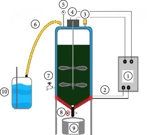
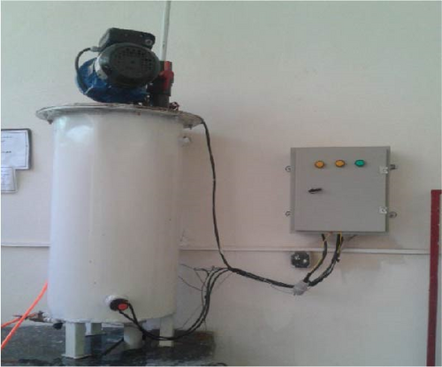
In this study, a 50-L, double-walled stainless steel reactor was used. An electric heater placed between the tank’s walls was used to supply the reactor’s required heat. Sampling was performed through the sampling valve at the digester’s bottom. Also, pH was detected daily using a pH meter (Sension 1 Company Hach). In addition, a shaft and electric motor with four stainless steel blades were installed to mix and blend the materials inside the bioreactor well. This agitator worked at 60 rpm. Figure 1 presents a schematic reactor diagram with different parts and an image of the pilot used in this study.
To ensure the integrity of the biogas reactor and prevent gas and water leakage, the digester underwent testing due to the pressure generated by the gas and organic matter within its chamber. Initially, pressure testing and pressure leak testing were conducted for the heater. Furthermore, silicone adhesives and gaskets were applied to the digester’s inlet to prevent any leakage or air infiltration, thereby maintaining anaerobic conditions.
2.3. Reactor Startup and Parameter Determination
The biogas pilot was operated in batch mode. To initiate and inoculate, the reactor was bioaugmented using anaerobic sludge from an industrial poultry wastewater treatment plant. Also, to load the digester with three different C/N ratios, 20, 30, and 40, the contents of organic carbon and nitrogen from the SHW and FVW were first detected. Subsequently, 1–2 mm pieces of the materials were prepared. The C/N ratio of the SHW and FVW mixture was then adjusted according to the pre-set values, and the runs were repeated to gain an optimum balance. The pilot was loaded with solid waste mixtures at three C/N ratios, 20, 30, and 40, and monitored until the biogas was detectably produced. The C/N ratio was kept fixed throughout the research, and the retention time was 40 days. At C/N = 20 ratio, the biogas composition—O2, CO, H2S, and CH4—was determined from the first day of loading to the last day of gas production using a gas detector (Gas Pro., Crowcon, Halma Plc., UK).
Furthermore, a TES-1370 (TES Electrical Electronic Corp., Taiwan) was employed to monitor CO2 volume. As mentioned previously, for suitable adaption of the bioreactor to anaerobic conditions, a microbial mass was applied before the loading stage, ensuring gas production from the first days of operation. Moreover, the volume of gas produced was detected daily by moving the reactor’s water column height.
Total solid (TS), volatile solid (VS), and electrical conductivity (EC) analyses were measured based on the procedure explained in the American Public Health Association (APHA) Standard Methods [26]. A pH meter was also used to measure the daily pH. The solid wastes’ total organic carbon (TOC) and total nitrogen (TN) content were determined before and after loading into the bioreactor.
2.4. Modeling
The modeling procedure is based on ANNs and three bioinspired optimizers: DE, BFO, and DA. Although ANNs are easy to use, their optimal parameter identification is a difficult task that must be solved to determine a good model that can efficiently work with the considered systems. The three optimizers considered in this work perform simultaneous topology identification and training.
2.4.1. Classical Modeling Approaches
Over the years, multiple models for AD have been developed. Some recent examples are (i) AD model no. 1 (ADM1), which includes several vital processes (hydrolysis, acidogenesis, acetogenesis, and methanogenesis) and parameters (concentration of organic matter, pH, temperature, hydraulic retention time, and loading rate); (ii) AD model no. 2 (ADM2), which is an improvement of ADM1; and (iii) AD model for municipal solid waste (ADM-MSW), an improvement of ADM1 that includes processes and parameters specific to municipal solid waste. One of the main advantages of these complex models is that they can simulate different feeds; however, they require many input parameters and an extensive set of experimental data [27]. To circumvent these drawbacks, simpler mathematical models focusing on single equations were developed. The work [28] effectively centralizes the main modeling strategies for AD systems. Since this manuscript focuses on the development of cumulative models, the following paragraphs will discuss only these models.
The cumulative models are mainly classified into exponential (with a data trend having no significant plateau at the end) and sigmoidal (that contains a lag factor) [28]. A few examples of cumulative models are presented in Table 2.
In Equations (1)–(5), y represents the cumulative production, A is the specific yield, µ is the maximum production rate, λ is the lag phase, v is the shape coefficient, and k is the rate constant.
The selection of the best model that fits the experimental data is a problem on its own. Overall, it was observed that the Gompertz model is best suited to simple substrates, with data following a reversed shape curve, while Richards is best suited to elongated S-shape or stepped curves [31].
2.4.2. Bioinspired Metaheuristics
DE is an optimization algorithm that evolves a series of potential solutions through a series of steps (mutation, crossover, and selection) until a stop criterion is reached. For the current work, the stop criterion is represented by the classical stop criterion encountered in evolutionary algorithms (the number of iterations reaches a maximum pre-defined value). The general schema of the algorithm has been presented in Figure 2.
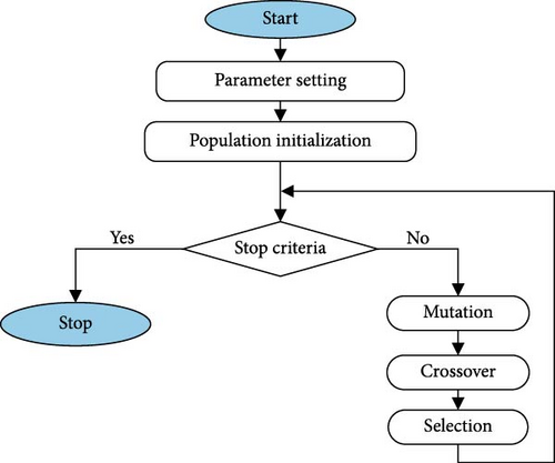
In the parameter setting step, all the algorithm parameters are initialized (maximum generation, population dimension, fluorine (F) which controls mutation, and chromium (Cr) which controls crossover). For the current work, a self-adaptive procedure is applied for F and Cr. The scope is to evolve these parameters simultaneously with the potential solution and, thus, to eliminate the necessity for manually tuning them. Moreover, the limits for each characteristic of the solutions are set. Finally, these limits are correlated with the problem being solved.
Based on the limits set in the previous step, the population is initialized using a random number generator. In this work, the normal distribution was used. Once initialized, the population was evaluated. In the mutation phase, the individuals are mutated using a differentiation procedure. In this work, the standard DE/rand/1 approach was used. This indicates that, to a randomly selected individual, a scaled differential term is added by the difference between two randomly chosen individuals.
In the crossover phase, the characteristics of the mutated population are combined with the ones from the current population. In this work, the binomial crossover was used. Finally, the trial population was evaluated to determine the performance. Finally, the trial and the current population were compared in the selection phase, and the individuals with the best loss were selected to form the next generation.
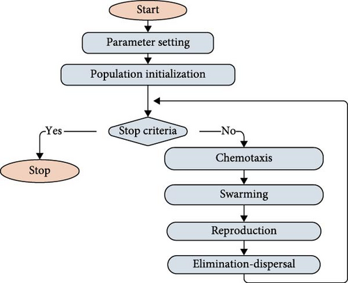
BFO performs the optimization process by simulating four operations (Figure 3): chemotaxis, swarming, reproduction, and elimination-dispersal. Similarly to the DE algorithm, these steps are repeated until a stop criterion is met. For example, in the chemotaxis step, the locomotion of bacteria is mimicked [32]. If the flagella of bacteria moves clockwise, it results in a forward movement; if it moves counterclockwise, then it tumbles, resulting in a movement in a random direction.
DA algorithm simulates dragonflies’ hunting and migration behavior [33] (Figure 4). This was performed in five steps: separation, alignment, cohesion, attraction, and distraction. Its actual position and the step vector (which represents a combination of all these steps) were used to update an individual.
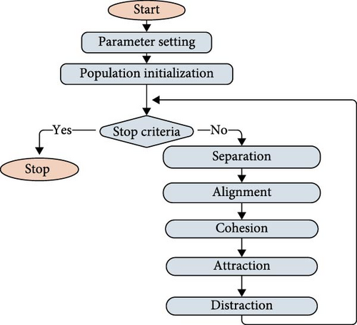
The separation was related to the avoidance of collisions in flight. On the other hand hand, alignment simulates the velocity matching of neighbors. Cohesion simulates the tendency of neighbors to concentrate toward the center of the neighborhood. Finally, attraction was focused on simulating going toward a food source, and distraction represents the flight response concerning an enemy. The exact relations used to model these behaviors can be encountered in [34].
2.4.3. Neuroevolution
The combination of the considered algorithms with ANNs belongs to the neuroevolution class. The advantage of using these algorithms instead of the classical learning strategies (e.g., backpropagation) is that several features can be simultaneously coevolved, and the evolutionary process can be more efficient [35]. Neuroevolution can be applied at different levels, and in this work, the optimizers were used to simultaneously evolve the topology (the hidden layers and its corresponding neurons), the connection weights (that are usually set through the training process that uses gradient-based strategies such as backpropagation algorithm), and node behavior (the type of activation functions and its associated parameters). If, in most cases, a single activation function is correlated with a type of layer, the proposed neuroevolutive strategy allows for selecting the activation function per neuron, thus identifying complex relations without extending the topology further.
The fully connected feed-forward multilayer perceptron represents the type of ANN used in this work. It was selected based on its efficiency in modeling different types of processes. For this type of network, as the topology increases, the number of parameters that must be considered for optimization increases almost exponentially. Thus, to balance performance and resources consumed, the maximum number of layers and neurons in each hidden layer was limited to 2, 20, and 10, respectively. These limitations were identified based on initial experiments that showed that the probability of finding a good model with the proposed strategy for a network with more than two layers is very low.
A direct encoding integrates all the ANN parameters considered for optimization with the actual structure required by the optimizers in their evolutive process. Thus, the phenotype (ANN parameters) is transformed into the genotype (vector of real numbers). During the evolutionary process for all algorithms, the performance of the associated ANN is required at specific steps to direct the search further. Thus, a decoding procedure to transform the genotype into the phenotype was applied in this case.
3. Results
3.1. AD: Methane Production
Figures 5 and 6 depict the methane and biogas production after 40 days. Initially, both methane and biogas volumes increased and subsequently declined during the process. For animal SHWs at C/N ratios of 20, 30, and 40, the reactor achieved a peak daily methane production of 14.2 L/day, 14.7 L/day, and 11.55 L/day, respectively. The corresponding biogas production reached 10.7, 11.4, and 8.93 L/day. Similarly, poultry SHWs exhibited an increase in performance (with a maximum daily methane production of 10.8, 11.5, and 10 L/day) followed by a decline. Overall, it is evident that animal wastes outperformed PWs in terms of methane production.
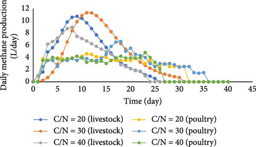
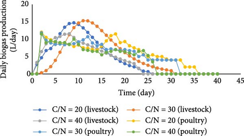
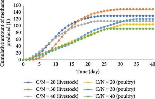
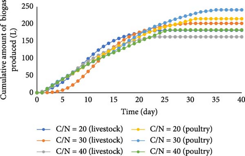
For the growth of anaerobic bacteria in the systems, the optimum C/N ratio lies between 20 and 30 [36]. However, in a study where onion juice and wastewater sludge were codigested using an anaerobic reactor, a C/N ratio of 15 was optimal and should be maintained throughout the process [37]. On the other hand, when corn was mixed with sewage sludge, the digestion process performed well at C/N = 15–18, but the AD process was not functional at ratios higher than 21. It should be pointed out that although adding FVW to SHW caused C/N to increase, as mentioned earlier, the C/N ratio ranged between the optimum levels, which was 20–30. Furthermore, at a ratio of 30, more methane and biogas are produced. In [38], the highest volume of biogas was produced when livestock and VPWs were codigested using a C/N ratio of 30.
After 21 days, biogas production reached its lowest level when C/N = 40; this accords with the observations of an investigation by Viswanath et al., in which the process of AD was tested on FVPWs, indicating that the produced biogas occurred within less than 5 days [39]. The major drawback of AD with FVW can be on account of the creation of a low pH environment, which negatively impacts the methanogenic phase. In another study, the degradation of organic matter came to a halt after 5 days due to a low pH (~4), consequently ceasing biogas production [40]. The digestion efficiency rate declines when the raw materials are high in lignocellulose and lignin. A decrease in active microorganisms in the digester results in a declining digestion rate. A reduction in methane production means that the concentration of CO2 increases in AD; in this case, acidogenic bacteria are more dominant than methanogens in biogas reactor, thereby decreasing pH and alkalinity and, in turn, reducing methane generation [41].
In the current research, the pH value inside the digester was measured. As seen from Figure 5, at the beginning of the process and the ratios of C/N = 20 and 30, animal wastes had pH = 6.3, which increased to 7.88 and 8.1 on the last day, respectively. Unlike the mentioned C/N ratios of 20 and 30, that pH ranged suitably, at C/N = 40, pH got acidic (pH = 4.94) and reached 5.91 during the reaction. Similar pH changes were observed for PWs (Figure 7). It has been documented that methanogens function better at a pH range between 6.4 and 7.2 [42]. Therefore, any fluctuation in pH may highly lead to decreased biogas production. A decline in pH acts as an inhibitory for methanogens. The process may fail if the pH reaches less than 5.5 [43]. It is worth noting that the reactor’s pH depends on the type of raw materials.
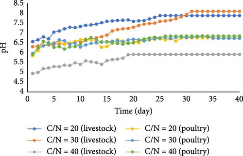
As observed, at C/N ratios of 20 and 30, the pH changes remained within the suitable range (7.5–8) for methanogens, with minimal fluctuations. This indicates a close relationship between the acidogenic and methanogenic phases, which helps maintain the pH around 7 without significant variations. However, at C/N ratio of 40, the pH decreased from 4.94 on the first day to 5.92 on the last day. This significant decrease in pH at C/N ratio of 40 can be attributed to the increased presence of fruit wastes, which are rich in hardly degradable lignocellulosic material [42].
The highest biogas production volume from animal SHWs was seen within 31 days. A related study, which tested different animal and agricultural waste ratios for biogas production, reported the highest production between 29 and 40 days [42]. The findings of [44] were consistent with the present study; it was also observed that biogas production stopped after 30 days at C/N = 30. The current study achieved the maximum biogas and methane output from poultry SHWs between 30 and 35 days. Other studies have reported similar durations of 25–45 days [45, 46].
3.2. Kinetic Modeling
The coefficients for the kinetic models are specific to each case (type of feedstock and C/N ratio). Thus, the nonlinear regression approach in Minitab software was applied to determine their values. The main idea is based on iteratively adjusting the coefficients to reduce the sum of squares for the residual errors (SSE). The algorithm used is Levenberg–Marquardt, with a maximum of 200 iterations and a 95% confidence level for all intervals. Tables 3 and 4 detail the statistical indicators obtained during the parameter optimization process for all five models presented in Table 1. In Tables 3 and 4, feed 1 indicates poultry, and feed 2 indicates livestock. S indicates how well the model describes the responses and how the best results are obtained at lower values. Moreover, the best results in each case are marked with bold.
| C/N | 20 | 30 | 40 | 20 | 30 | 40 |
|---|---|---|---|---|---|---|
| Feed | 1 | 1 | 1 | 2 | 2 | 2 |
| Gompertz | ||||||
| Iterations | 18 | 18 | 21 | 35 | 50 | 50 |
| Final SSE | 6.9E + 01 | 9.2E + 01 | 1.3E + 02 | 2.6E + 00 | 2.6E − 06 | 2.5E + 01 |
| MSE | 2.5E + 00 | 2.9E + 00 | 5.4E + 00 | 1.2E − 01 | 1.0E − 07 | 1.2E + 00 |
| S | 1.6E + 00 | 1.7E + 00 | 2.3E + 00 | 3.4E − 01 | 3.1E − 04 | 1.1E + 00 |
| Logistic | ||||||
| Iterations | 22 | 34 | 22 | 26 | 23 | 23 |
| Final SSE | 2.5E + 02 | 1.6E + 02 | 2.8E + 02 | 1.6E + 02 | 2.9E + 02 | 2.1E + 02 |
| MSE | 8.9E + 00 | 5.0E + 00 | 1.2E + 01 | 7.2E + 00 | 1.1E + 01 | 1.0E + 01 |
| S | 3.0E + 00 | 2.2E + 00 | 3.4E + 00 | 2.7E + 00 | 3.3E + 00 | 3.2E + 00 |
| Richards | ||||||
| Iterations | 132 | 15 | 200 | 29 | 200 | 200 |
| Final SSE | 6.9E + 00 | 8.7E + 01 | 1.4E + 01 | 1.9E + 00 | 2.7E − 06 | 2.5E + 01 |
| MSE | 2.6E − 01 | 2.8E + 00 | 6.2E − 01 | 9.0E − 02 | 1.0E − 07 | 1.3E + 00 |
| S | 5.1E − 01 | 1.7E + 00 | 7.9E − 01 | 3.0E − 01 | 3.2E − 04 | 1.1E + 00 |
| First-order | ||||||
| Iterations | 38 | 200 | 200 | 22 | 41 | 23 |
| Final SSE | 1.6E + 02 | 9.7E + 02 | 1.1E + 02 | 2.5E + 03 | 6.4E + 03 | 7.4E + 02 |
| MSE | 5.6E + 00 | 3.0E + 01 | 4.2E + 00 | 1.1E + 02 | 2.3E + 02 | 3.5E + 01 |
| S | 2.4E + 00 | 5.4E + 00 | 2.1E + 00 | 1.0E + 01 | 1.5E + 01 | 5.9E + 00 |
| Fitzhugh | ||||||
| Iterations | 200 | 200 | 200 | 200 | 200 | 200 |
| Final SSE | 3.8E + 03 | 7.5E + 03 | 2.3E + 04 | 1.2E + 04 | 2.2E + 04 | 6.3E + 03 |
| MSE | 1.4E + 02 | 2.3E + 02 | 9.6E + 02 | 5.6E + 02 | 8.2E + 02 | 3.2E + 02 |
| S | 1.2E + 01 | 1.5E + 01 | 3.1E + 01 | 2.4E + 01 | 2.9E + 01 | 1.8E + 01 |
- Abbreviations: C/N, carbon-to-nitrogen; MSE, mean squared error; S, standard error of the regression; SSE, sum of squares for the residual errors.
| C/N | 20 | 30 | 40 | 20 | 30 | 40 |
|---|---|---|---|---|---|---|
| Feed | 1 | 1 | 1 | 2 | 2 | 2 |
| Gompertz | ||||||
| Iterations | 20 | 15 | 16 | 14 | 15 | 15 |
| Final SSE | 5.2E + 01 | 2.2E + 02 | 9.3E + 01 | 1.9E + 00 | 2.3E − 06 | 2.3E − 06 |
| MSE | 1.9E + 00 | 6.9E + 00 | 3.9E + 00 | 8.8E − 02 | 1.0E − 07 | 1.0E − 07 |
| S | 1.4E + 00 | 2.6E + 00 | 2.0E + 00 | 3.0E − 01 | 2.9E − 04 | 2.9E − 04 |
| Logistic | ||||||
| Iterations | 17 | 18 | 23 | 19 | 15 | 19 |
| Final SSE | 1.8E + 02 | 4.1E + 02 | 2.4E + 02 | 1.9E + 01 | 4.8E + 01 | 3.9E + 01 |
| MSE | 6.5E + 00 | 1.3E + 01 | 1.0E + 01 | 8.6E − 01 | 1.8E + 00 | 2.0E + 00 |
| S | 2.6E + 00 | 3.6E + 00 | 3.2E + 00 | 9.3E − 01 | 1.3E + 00 | 1.4E + 00 |
| Richards | ||||||
| Iterations | 115 | 200 | 200 | 12 | 94 | 120 |
| Final SSE | 2.9E + 01 | 8.7E + 01 | 3.5E + 00 | 4.3E − 01 | 2.3E − 06 | 2.5E − 01 |
| MSE | 1.1E + 00 | 2.8E + 00 | 1.6E − 01 | 2.0E − 02 | 1.0E − 07 | 1.3E − 02 |
| S | 1.0E + 00 | 1.7E + 00 | 4.0E − 01 | 1.4E − 01 | 3.0E − 04 | 1.2E − 01 |
| First-order | ||||||
| Iterations | 19 | 22 | 19 | 20 | 40 | 20 |
| Final SSE | 2.4E + 02 | 1.1E + 02 | 5.5E + 01 | 3.7E + 02 | 1.0E + 03 | 7.9E + 01 |
| MSE | 8.3E + 00 | 3.2E + 00 | 2.2E + 00 | 1.6E + 01 | 3.7E + 01 | 3.8E + 00 |
| S | 2.9E + 00 | 1.8E + 00 | 1.5E + 00 | 4.0E + 00 | 6.1E + 00 | 1.9E + 00 |
| Fitzhugh | ||||||
| Iterations | 200 | 200 | 200 | 200 | 200 | 200 |
| Final SSE | 5.1E + 03 | 5.4E + 03 | 1.5E + 04 | 1.5E + 04 | 2.3E + 04 | 1.4E + 04 |
| MSE | 1.8E + 02 | 1.7E + 02 | 6.4E + 02 | 7.0E + 02 | 8.4E + 02 | 7.0E + 02 |
| S | 1.3E + 01 | 1.3E + 01 | 2.5E + 01 | 2.6E + 01 | 2.9E + 01 | 2.7E + 01 |
- Abbreviations: C/N, carbon-to-nitrogen; MSE, mean squared error; S, standard error of the regression; SSE, sum of squares for the residual errors.
As shown in Tables 3 and 4, the best results for livestock feed were obtained with the Richards models at all C/N ratios studied for both methane and CO2. On the other hand, for poultry feed, at a C/N ratio of 20, for both methane and CO2, the best fit was the Richards model and the other rations with the Gompertz model. The values for the best model parameters in each case have been presented in Table 5.
| C/N | 20 | 30 | 40 | 20 | 30 | 40 |
|---|---|---|---|---|---|---|
| Feed | 1 | 1 | 1 | 2 | 2 | 2 |
| Methane | ||||||
| A | 166.705 | 134.737 | 2038.97 | 132.967 | 52.381 | 119.311 |
| v | −0.679 | 0.175 | −0.95 | 0.05 | — | — |
| μ | −46.53 | 1.901 | −1911.99 | 1.356 | 11.1378 | 8.378 |
| λ | 1.694 | 4.623 | 1.29 | 3.548 | 5.99 | 2.25 |
| CO2 | ||||||
| A | 104.379 | 134.74 | 94.34 | 55.7572 | 61.7759 | 51.6649 |
| v | −0.456 | −0.94 | −0.98 | 0.1837 | — | — |
| μ | −15.581 | −1841.1 | −9247.65 | 1.7022 | 4.6128 | 3.3207 |
| λ | 1.027 | 0.32 | 0.91 | 3.1992 | 5.99 | 1.72 |
- Abbreviations: C/N, carbon-to-nitrogen; CO2, carbon dioxide.
The core difficulty in modeling the cumulative methane and CO2 with single-equation models relies on the necessity for determining the coefficients and applying the equation for each case. Moreover, selecting the starting values for parameter identification can significantly impact the performance. One significant disadvantage is that the models cannot efficiently predict the cumulative response for untested cases, and additional measurements must be performed. In this context, ANN modeling is a viable alternative to solve the abovementioned issues.
3.3. ANN Modeling
The gathered data underwent a preprocessing step to determine the best model for the considered process: randomization, data splitting (75% training and 25% testing), and normalization. The normalization procedure uses the min–max strategy [47] and controls the influence of inputs with large scales on the output.
Afterward, the selected optimizers were applied with a population dimension of 50 individuals. Considering the different strategies performed by these algorithms during the search, the stop condition usually used (the number of iterations) was replaced by the number of function evaluations (100,000). In this manner, all the algorithms stop simultaneously, allowing a better comparison of their performance for the analyzed system.
Since all three algorithms selected have a stochastic nature, they were run 50 times, the best model being selected as the one with the highest fitness, which was computed based on the mean squared error (MSE) in the training phase. Two cases were considered: methane and CO2. These outputs were determined as a function of feedstock type (encoded with 1 for poultry slaughterhouse and 2 for livestock slaughterhouse), process duration, C/N ratio, and pH. The statistics of the models determined in each case by the three considered optimizers are presented in Table 6.
| Output | Algorithm | Statistic | Fitness | MSE train | MSE test | R2 train | R2 test | Topology |
|---|---|---|---|---|---|---|---|---|
| CO2 | DE | Best | 450.5481 | 0.00222 | 0.001557 | 0.985204 | 0.990609 | 4:04:01 |
| Worst | 16.81965 | 0.059454 | 0.058671 | 0.569376 | 0.613331 | 4:17:01 | ||
| Average | 126.8643 | 0.017563 | 0.018493 | 0.880189 | 0.890836 | — | ||
| BFO | Best | 1294.436 | 0.000773 | 0.000552 | 0.995362 | 0.997228 | 4:06:01 | |
| Worst | 598.6854 | 0.00167 | 0.001285 | 0.988737 | 0.992254 | 4:06:01 | ||
| Average | 933.9173 | 0.001107 | 0.001058 | 0.992729 | 0.994352 | — | ||
| DA | Best | 234.1874 | 0.00427 | 0.003911 | 0.970934 | 0.976624 | 4:10:01 | |
| Worst | 49.64292 | 0.020144 | 0.022323 | 0.904477 | 0.906418 | 4:07:01 | ||
| Average | 99.16074 | 0.011241 | 0.011332 | 0.936524 | 0.947736 | — | ||
| Methane | DE | Best | 223.6855 | 0.004471 | 0.003625 | 0.978024 | 0.984752 | 4:09:01 |
| Worst | 20.65734 | 0.048409 | 0.046381 | 0.672458 | 0.693642 | 4:07:01 | ||
| Average | 56.91997 | 0.023205 | 0.0218 | 0.876898 | 0.89738 | — | ||
| BFO | Best | 580.4406 | 0.001723 | 0.001598 | 0.990223 | 0.993111 | 4:04:01 | |
| Worst | 174.0859 | 0.005744 | 0.004862 | 0.965291 | 0.973547 | 4:05:01 | ||
| Average | 310.2027 | 0.003449 | 0.00299 | 0.979423 | 0.983971 | — | ||
| DA | Best | 107.7184 | 0.009283 | 0.007852 | 0.944147 | 0.957608 | 4:12:01 | |
| Worst | 41.22967 | 0.024254 | 0.016735 | 0.853664 | 0.915876 | 4:10:01 | ||
| Average | 65.91744 | 0.016196 | 0.015249 | 0.911191 | 0.926564 | — | ||
- Abbreviations: BFO, Bacterial Foraging Optimization; CO2, carbon dioxide; DA, Dragonfly Algorithm; DE, Differential Evolution; MSE, mean squared error.
A comparison with existing models indicates that the obtained ANNs have similar performance. For example, an ANN determined for the codigestion tea factory waste (TFW) and spent tea waste (STW) had an R2 of 0.9997 in the training phase [48]. The ANN had a single hidden layer with 50 neurons, was trained with Bayesian regularization, and considered as inputs the ratios of substrates. At the same time, the outputs represented the cumulative methane yield for the duration of the entire process (49 outputs). Another ANN model focusing on the biogas quantity prediction based on pH, digestion time, and C/N ratio for the codigestion of seed cake of Karanja and cattle dung has an R2 in the testing phase varying from 0.991 to 0.998 for different samples [49].
By analyzing Table 6, it can be observed that BFO provided the best results for both outputs, indicating that this algorithm is best suited to explore the search space for the considered process. Regarding performance indexes, the average absolute percentual error (AAPE) for the entire dataset was computed in all cases for both ANN and kinetic models (Table 7). This was done to compare the two types of models in similar conditions, especially considering that the kinetic parameters are set using all the available experimental points. For methane, the big AAPE for ANN-DA is given by the fact that, for a reduced number of cases, the difference in predictions is relatively high, which results in a higher AAPE (e.g., experimental 2.5 L and predicted 17.54 L, which results in 602.9% AAPE).
| Output | Model | AAPE (%) |
|---|---|---|
| CO2 | Kinetic | 8.39 |
| ANN-DE | 12.38 | |
| ANN-BFO | 8.32 | |
| ANN-DA | 20.11 | |
| Methane | Kinetic | 16.34 |
| ANN-DE | 24.66 | |
| ANN-BFO | 12.45 | |
| ANN-DA | 46.62 | |
- Abbreviations: AAPE, average absolute percentual error; ANN, artificial neural network; BFO, Bacterial Foraging Optimization; CO2, carbon dioxide; DA, Dragonfly Algorithm; DE, Differential Evolution; MSE, mean squared error.
A comparison between the experimental data and the predictions obtained with the best models has been presented in Figure 8 for CO2 and Figure 9 for methane. As can be observed, for most experimental points, all models’ predictions follow a similar trend. This indicates that all models captured the process dynamic. However, in terms of AAPE indicator, ANN-BFO outperforms all other models. Moreover, for the testing data (which for the kinetic models were used to determine the parameters, while for the ANNs represent unseen data), the kinetic models seem to have some difficulties for a few points in the case of methane predictions, a fact that further underlines the performance of the ANN-BFO model.
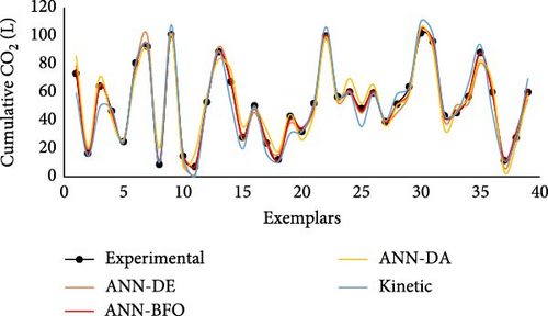
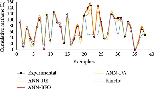
After selecting the best models, they can be further used to generate predictions. To these means, the mathematical relations that describe the ANN for cumulated are represented by Equations (S1)–(S12) and (S13)–(S22) for cumulated methane. These relations are presented in Python format and can be used as such. These models can be applied by the end users of the proposed system to correlate the consumption with the peak production and to efficiently identify the biogas production when different C/N ratios were used at similar pH variations.
4. Conclusions
In this work, biogas production using two sources (animal slaughterhouse and poultry slaughterhouse) was studied, modeled, and optimized. The experimental analysis showed that the efficiency of the process is influenced by the raw materials used. The best results were obtained for the poultry slaughterhouse for a process duration of 30–35 days. Moreover, to establish a model that can simulate the process and determine the cumulative biogas production in different conditions, ANNs were applied with three optimization algorithms. The obtained models correlated well with the experimental data, indicating that the determined ANNs can simulate the system in various conditions. Therefore, these models can be further used in the optimization process to identify the best conditions and ratios that can lead to the highest efficiency and can also be used for planning consumption to correlate with the production peak, considering the two types of feedstocks.
Conflicts of Interest
The authors declare no conflicts of interest.
Funding
The work of E.N.D. and G.D.S. was funded by UEFISCDI (grant number PCE 58/2021).
Supporting Information
Additional supporting information can be found online in the Supporting Information section.
Open Research
Data Availability Statement
The data can be available upon request.


