We propose a new CQ algorithm which combines the inertial technique and correction terms for solving the split feasibility problem with multiple output sets in Hilbert spaces. Under suitable conditions, we prove the weak convergence. Moreover, we demonstrate the linear convergence when the split feasibility problem with multiple output sets satisfies some bounded linear regularity property. Finally, numerical experiments are conducted to demonstrate superiority of our method over related inertial CQ method and classical CQ method for the split feasibility problem with multiple output sets.

1. Introduction

Our objective in this paper is to propose a fast algorithm to solve the split feasibility problem with multiple output sets (SFPwMOS). Find an element x^∗ in real Hilbert spaces H and H_i, i = 1, ⋯, N such that

()

where C and Q_i are nonempty, closed, and convex subsets of H and H_i, i = 1, ⋯, N, and A_i : H⟶H_i, i = 1, ⋯, N are nonzero bounded linear operators. When N = 1, the problem (SFPwMOS) will be the split feasibility problem (SFP):

()

The SFP was first introduced by authors in [1], which was widely studied by many authors over a long period of time. In recent years, many versions of CQ methods for solving the SFP (2) have been introduced and analyzed [2–7]. Byrne [2] introduced the first applicable and most celebrated method called the well-known CQ-algorithm:

()

where P_C and P_Q represent the metric projections onto C and Q, respectively, the step size λ_λ ∈ (0, 2/‖A‖²), and ‖A‖² is the spectral radius of the matrix; A^TA(A^T denotes the adjoint operator of A).

In comparison to the basic algorithm, the algorithm incorporating inertial extrapolation steps have been demonstrated to achieve a faster convergence rate and require few iterations in theory and numerical experiments [8–13]. In [12], Dang et al. investigated CQ algorithms with inertial extrapolation steps.

()

and

()

where w^k = x^k + α_k(x^k − x^k−1), β_k ∈ (0, 1), λ ∈ (0, 2/‖A‖²). Shehu and Gibali [13] proposed a new inertial relaxed method:

()

where

, and γ > 0, l ∈ (0, 1), μ ∈ (0, 1), m_k is the smallest non-negative integer

. Moreover, inertial techniques have also achieved great success in real-world applications [14–16].

The (SFPwMOS) problem has attracted a lot of scholars to analyze and study [17–22]. Dang et al. [23] defined the function

as follows:

()

It is not difficult to see that an element x^∗ is a solution of the SFPwMOS if and only if it is the solution of the following problem:

()

which is equivalent to

()

where N_C(x) is the normal cone of C at point x. It implies that

()

where α is an arbitrary positive real number.

Due to the advantage of accelerating convergence, the application of inertial technology in solving SFPwMOS problems has become increasingly popular. Taddele et al. [24] introduced an extended inertial Halpern-type ball-relaxed CQ algorithm and proved a strong convergence of the sequence generated by the proposed algorithm under some mild assumptions. Okeke et al. [25] proposed two inertial accelerated algorithms which did not require prior knowledge of operator norm. Dang et al. [23] used a self-adaptive inertial viscosity projection algorithm (SIVP) for SFPwMOS:

()

where

Inspired by the authors in [7, 11], in order to further enhance the convergence speed of the already studied CQ algorithms, we propose new inertial CQ algorithm correction terms for problem (1). Our main contributions of this paper are outlined as follows:

i.
Our algorithm employs correction terms and self-adaptive step-size λ_k in each iterive step to improve the convergence
ii.
Under some mild assumptions, we analyze the weak and linear convergence of the generated sequence

The rest of the paper is organized as follows: In Section 2, we present fundamental concepts and lemmas. Section 3 proposes an inertial CQ algorithm with correction terms for solving the SFPwMOS problem and shows its weak and linear convergence. In Section 4, we test the efficacy of the algorithm by two numerical experiments. Finally, some conclusions are given in Section 5.

2. Preliminaries

We recall some definitions and basic results that will be used in Section 3.

Suppose H is a real Hilbert space. We say that

a.
Nonexpansive if ‖Tx − Ty‖≤‖x − y‖, for all x, y ∈ H;
b.
Firmly nonexpansive if for all x, y ∈ H.

Equivalently, ‖Tx − Ty‖² ≤ 〈x − y, Tx − Ty〉 for all x, y ∈ H.

From [26], T is firmly nonexpansive if and only if I − T is firmly nonexpansive.

The operator P_C is called the metric projection of H onto C; if given x ∈ H, there exists a unique point P_C(x) ∈ C such that

()

We know from [27] that P_C is a firmly nonexpansive mapping of H onto C. Furthermore,

()

and

()

Therefore,

()

A function

is said to be convex if f(λx + (1 − λ)y) ≤ λf(x) + (1 − λ)f(y), ∀λ ∈ (0, 1), ∀x, y ∈ H. Also f is convex on H, and differentiable implies

()

We say that g ∈ H is a subgradient of

at x provided

()

and f is lower semicontinuous (1sc) at x if y^k⟶y implies f(y) ≤ lim inf_k⟶∞ f(y^k) and f is lower semicontinuous on H if it is lower semicontinuous at every point y ∈ H.

Lemma 1. The following statements hold in:

i.
for all x, y ∈ H;
ii.
for all x, y ∈ H;
iii.
.

3. Algorithm and Convergence

This section first introduces our inertial CQ algorithm with correction terms, then discusses its weak convergence and linear convergence rate.

Algorithm 1. Inertial CQ algorithm with correction terms.

Choose ρ_k ∈ (0, 4), α_k ∈ [0, 1), δ ∈ [0, 1), w⁻², w⁻¹ ∈ H, x⁻¹, x⁰ ∈ C. Set k≔0.

()

where

Remark 1. Obviously, implies that . To ensure that λ_k is well-defined, we assume that ∇g(W^k) ≠ 0 in our convergence analysis.

3.1. Weak Convergence Analysis

To demonstrate the weak convergence and linear convergence rate, we need the following assumption and lemma.

Assumption 1. Throughout our convergence analysis, we assume that

a.
0 < lim inf ρ_k≤ limsup ρ_k < 4;
b.
The solutions set S is nonempty.

Lemma 2. Both {w^k} and {x^k} generated by Algorithm 1 are bounded under Assumption 1.

Proof 1. For the rest of the convergence analysis of this paper, we define

()

From Algorithm 1, we have

()

Then, for any

, that is,

, we have

()

Consequently, since

is firmly nonexpansive, from (14), we obtain

()

Therefore,

()

Now, from y^k = x^k + δ(w^k−1 − x^k), we obtain x^k = (y^k − δw^k−1/1 − δ) and y^k − w^k−1 = (1 − δ)(x^k − w^k−1). Then, from Lemma 1 (iii), we have

()

We furthermore obtain from (23) and (24) that

()

By Lemma 1 (iii), we obtain

()

Making use of (25) and (26), we obtain,

()

where

()

Applying (25) in (26), we obtain

()

Rearranging the above inequality, we obtain

()

Thus,

()

Therefore,

()

Define

()

Then, (33) becomes

()

Hence, β_k ≥ 0 and β_k+1 ≤ β_k since α_k ∈ [0, 1) and δ ∈ [0, 1). Furthermore, we have from (34) that lim_k⟶∞ β_k exists and {β_k} is bounded. So, {y^k} is bounded from (33).

Theorem 1. The sequence {x^k} generated by Algorithm 1 converges weakly to a point in when Assumption 1 is satisfied.

Proof 2. Since {x^k} is bounded from Lemma 2, we have that {x^k} has at least one accumulation point v ∈ H. Suppose such that . We show that . Since C is a closed and convex subset of H, then C is weakly closed. Now, since and , it then follows that v ∈ C. To show that , we consider these two cases.

Case A: Assume that α_k = 0 in (10). Then, our proposed algorithm reduces to

()

Hence, (33) becomes

()

from which we obtain that {x^k} is bounded. We then obtain from (34) that

()

which implies (if δ ∈ (0, 1))

()

and

()

If δ = 0, k⟶∞, then x^k = y^k and lim_k⟶∞ ‖x^k − y^k‖ = lim_k⟶∞ ‖y^k − x^k−1‖ = 0. We furthermore obtain from (34) that

()

Since

, we have

. Then,

()

Therefore,

is bounded. From (40), we have

. Since

is bounded, there exists a subsequence {x^k} of {x^k}, ∀x^k ∈ H₁ which is weakly lower semicontinuous, and we have

()

Hence, A_iv ∈ Q_i, i⟶∞.

Case B: Assume 0 < d₁ ≤ α_k ≤ α_k+1 ≤ d₂ < 1. Then, we have from (34) that (if ∈(0, 1))

()

Consequently, we have from (19) and (20) that

()

and

()

So, ‖w^k − x^k‖ ≤ ‖w^k − y^k‖ + ‖y^k − x^k‖⟶0, k⟶∞. Since {y^k} is bounded, we have

such that

. Following a similar approach as in Case A, we have that

. Now, suppose

()

Observe that

()

and

()

Therefore,

()

Hence,

()

Since lim_k⟶∞ ‖y^k − y^k−1‖ = 0 and {x^k} is bounded, we obtain

and

. By the existence of the limit of a_k, we have from (50), lim_k⟶∞ ‖y^k − z‖ exists

. Furthermore,

()

implies that lim_k⟶∞ ‖x^k − z‖ exists

. We then conclude that {x^k} converges weakly to a point in

by Opial’s lemma [28].

Remark 2. We obtain boundedness and convergence of {x^k} generated by Algorithm 1 using Assumption 1 without using the on-line rule: Choose α_k such that and

()

where

and α ≥ 0. The on-line rule (52) has been assumed severally by many authors whenever inertial CQ algorithm is studied (see, for example, [12, 22, 29, 30]). Consequently, the assumption “

” is dispensed with in our Lemma 2 and Theorem 1.

3.2. Linear Convergence

In this subsection, we give the linear convergence rate of the sequences generated by Algorithm 1 under the following bounded linear regularity property of SFPwMOS:

For any r > 0 such that

, where

and

is a closed metric ball, there exists γ_r > 0 such that

()

where d_S(x)≔inf_y∈S ‖x − y‖, x ∈ H. It was shown in [31] that if C and Q_i are polyhedron, then SFPwMOS satisfies the bounded linear regularity property. For more details of sufficient conditions for the bounded linear regularity property, see ([31], Proposition 2.5).

Theorem 2. Let . Assuming that the SFPwMOS problem satisfies the bounded linear regularity property. {x^k} generated by Algorithm 1 converges to a solution R-linearly when Assumption 1, α_k = 0, δ = 0, ∀k ≥ 0, are fulfilled.

Proof 3. From (15), we have

()

By Lemma 2, we have that w_k is bounded. Therefore, ∃r > 0 such that . Using the condition that SFPwMOS fulfills the bounded linear regularity property, it follows that ∃γ_r > 0 such that

()

We then obtain from (54) that

()

for each

()

We then obtain from (26) that ∀k ≥ k₂,

()

if α_k = 0,then (58) becomes (noting (10))

()

Thus, ∀k ≥ k₂,

()

if and only if

()

Since 0 < lim inf ρ_k ≤ limsup ρ_k < 4, we obtain

()

Hence,

()

Consequently,

()

So, ∃k₃ ≥ k₂ such that

()

if δ = 0 (36), then it becomes (noting (19))

()

Then, it is easy to see that {x^k} converges linearly to z.

4. Numerical Experiment

In this section, we examine two numerical experiments to compare the effects of Algorithm 1, classic CQ in [2] and SIVP in [23]. All the codes are written in MATLAB and are performed with RAM 8 GB and Intel(R) Core (TM) i7-8265U CPU @ 1.60 GHz. We consider the following problems:

Example 1. Find a point x^∗ such that

()

where the sets C and Q_i, i = 1, 2 and the linear bounded operators A_i, i = 1, 2 are defined as

()

In the experiments, we use E_k ≤ ϵ as the stopping criteria, where E_k≔TOL_k,

()

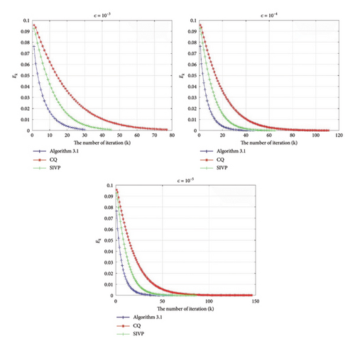
where ϵ is a small enough positive number. Note that if E_k = 0, then x^k ∈ S.

Firstly, for Algorithm 1 we take α_k = 0.1, ρ_k = 3.0, δ = 0.1, w⁻¹ = (0.2, 0.3, 0.5), w⁻² = (0.3, 0.6, 0.9); in [23] for CQ, we take λ_k = 1, and in [23] for SIVP, we take λ_k = 1, t_k = 0, ρ_k = 3.0 and α_k = 0.1. The ϵ = 10⁻³, 10⁻⁴, 10⁻⁵, respectively. Then, we chose initial points x⁻¹ = (0, 0.1, 0), x⁰ = (0, 0.1, 0) for Algorithm 1, SIVP and x⁰ = (0, 0.1, 0) for CQ to compare the experimental effects of the three groups. The behavior values of the function E_k with different ε are listed in Table 1, where “Iter.” and “Cpu” denote the number of iterations and cpu time in seconds.

We also plot E_k versus the number of iterative in Figure 1.

Obviously, from Table 1 and Figure 1, Algorithm 1 takes much less iterations and computing time than SIVP and CQ algorithm.

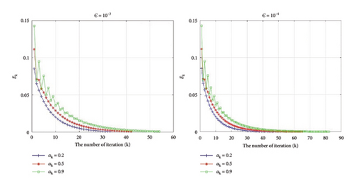
Secondly, select ρ_k = 3, δ = 0.1, w⁻¹ = (0.2, 0.3, 0.5), w⁻² = (0.3, 0.6, 0.9) for the same initial points x⁻¹ = (0, 0.1, 0), x⁰ = (0, 0.1, 0), and we test the results for different α_k and ε for Algorithm 1.

The behavior of the function Ek in Table 2 is described in Figure 2.

From Table 2 and Figure 2, we can see that as ε increases, the iteration steps decrease but when α_k increases, the iteration steps still increase.

Table 1. The results of Algorithm 1 and SIVP and CQ algorithm for different ε.

ε	10⁻³		10⁻⁴		10⁻⁵
Algorithm 1	Inter. = 30	Cpu = 0.01	Inter. = 47	Cpu = 0.031	Inter. = 63	Cpu = 0.055
Algorithm 1	TOL_k = 9.4237E − 04		TOL_k = 8.8209E − 05		TOL_k = 9.3113E − 06

SIVP	Inter. = 45	Cpu = 0.012	Inter. = 65	Cpu = 0.042	Inter. = 85	Cpu = 0.072
SIVP	TOL_k = 9.5199E − 04		TOL_k = 9.31750E − 05		TOL_k = 9.3560E − 06

CQ	Inter. = 77	Cpu = 0.16	Inter. = 111	Cpu = 0.052	Inter. = 146	Cpu = 0.096
CQ	TOL_k = 9.6469E − 04		TOL_k = 9.9749E − 05		TOL_k = 9.8560E − 06

Details are in the caption following the image — **Figure 1**
Open in figure viewer PowerPoint

Comparison with different ε for Algorithm 1 and CQ.

Table 2. The results of Algorithm 1 with different α_k and ε.

ε	α_k = 0.2	α_k = 0.5	α_k = 0.9
10⁻³	Iter. = 33	Iter. = 42	Iter. = 54
10⁻³	TOL = 9.7664E − 04	TOL = 9.7212E − 04	TOL = 9.3819E − 04

10⁻⁴	Iter. = 51	Iter. = 65	Iter. = 82
10⁻⁴	TOL = 9.6424E − 05	TOL = 9.1123E − 05	TOL = 9.5076E − 05

Example 2. Consider the following monotone inclusion problem [32]:

()

where

and

. Define the linear continuous operator L : L²([0, 2π])⟶L²([0, 2π]) as

()

The projection onto the set C can be computed as

()

The projection onto the set Q can be computed as

()

Let

()

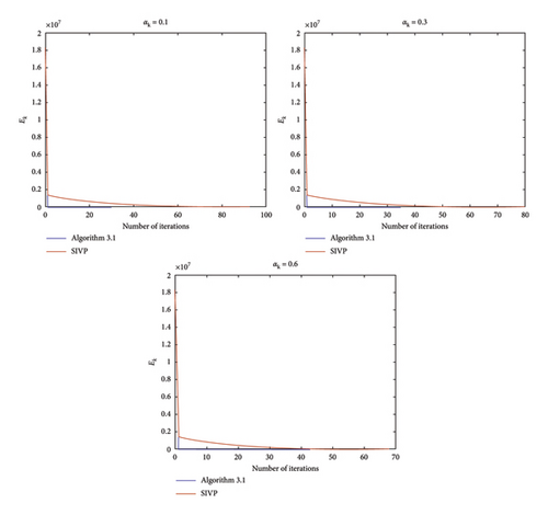
be the stopping criterion. Table 3 and Figure 3 present the numbers of iterations needed by Algorithm 1 and SIVP (here, we do not consider the general CQ algorithm since it is no-inertial version). Set ρ_k = 3.0 for every k ≥ 0, δ = 0.9, λ = 1, t_k = 0. Select inertial factors α_k = 0.1, 0.3, 0.6, respectively. The specific results are shown in Table 3.

Figure 3 plots the trend of E_k with the iteration for α_k = 0.1, 0.3, 0.6, with initial points (x⁰, x⁻¹) = (t³, t³) for Algorithm 1 and SIVP, respectively.

Table 3 and Figure 3 also show that our algorithm performs better than SIVP.

Based on the above two numerical experiments, we can see that the application of the inertial technique and correction terms can improve the performance of the algorithm.

Table 3. Comparison of different inertial factors α_k by Algorithm 1 and SIVP.

Iter. for Algorithm 1							Iter. for SIVP
x⁰	x⁻¹	w⁻¹	w⁻²	α_k = 0.1	α_k = 0.3	α_k = 0.6	x⁰	x⁻¹	α_k = 0.1	α_k = 0.3	α_k = 0.6
t²	t	t²/5	t²/5	16	18	21	t²	t	44	31	25
t²	t²	t²/5	t²/5	18	19	22	t²	t²	53	47	43
t³	t²	t²/5	t²/5	29	30	35	t³	t²	86	72	67

5. Conclusions

In this paper, we propose an inertial CQ algorithm with correction terms for solving SFPwMOS. Under some suitable conditions, we show the weak convergence and linear convergence results by the bounded linear regularity property. Two numerical experiments show that our algorithm performs better than other algorithms.

Conflicts of Interest

The authors declare no conflicts of interest.

Author Contributions

Yang Liu, Yazheng Dang, and Kang Liu wrote the main manuscript text. All authors carried out all the experiments and reviewed the manuscript.

Funding

This work was supported by the National Key Research and Development Program of China (2023YFC3306100, 2023YFC3306105, 2023YFC3306103), Major Projects of the National Social Science Foundation (20&ZD199), Shanghai Philosophy and Social Science Planning Project (2023EFX011), National Natural Science Foundation of China under grants 72071130 and 71901145, and Humanities and Social Sciences Research Project of the Ministry of Education under grant 20YJC820030.

Open Research

Data Availability Statement

The data used to support the findings of this study are included within the article.

References

1 Censor Y. and Elfving T., A Multiprojection Algorithm Using Bregman Projections in a Product Space, Numerical Algorithms. (1994) 8, no. 2, 221–239, https://doi.org/10.1007/bf02142692, 2-s2.0-0000424337.
10.1007/BF02142692
Google Scholar
2 Byrne C., Iterative Oblique Projection Onto Convex Sets and the Split Feasibility Problem, Inverse Problems. (2002) 18, no. 2, 441–453, https://doi.org/10.1088/0266-5611/18/2/310, 2-s2.0-0036538286.
10.1088/0266-5611/18/2/310
Web of Science® Google Scholar
3 Censor Y. and Lent A., An Iterative Row-Action Method for Interval Convex Program-Ming, Journal of Optimization Theory and Applications. (1981) 34, no. 3, 321–353, https://doi.org/10.1007/bf00934676, 2-s2.0-0019587748.
10.1007/bf00934676
Google Scholar
4 Gibali A., Liu Li-W., and Tang Yu-C., Note on the Modified Relaxation Cq Algorithm for the Split Feasibility Problem, Optimization Letters. (2018) 12, no. 4, 817–830, https://doi.org/10.1007/s11590-017-1148-3, 2-s2.0-85018361148.
10.1007/s11590-017-1148-3
Web of Science® Google Scholar
5 Jouymandi Z. and Moradlou F., Extragradient and Linesearch Methods for Solving Split Feasibility Problems in Hilbert Spaces, Mathematical Methods in the Applied Sciences. (2019) 42, no. 12, 4343–4359, https://doi.org/10.1002/mma.5654, 2-s2.0-85066129521.
10.1002/mma.5654
Web of Science® Google Scholar
6 López G., Martín-Márquez V., Wang F., and Xu H.-K., Solving the Split Feasibility Problem Without Prior Knowledge of Matrix Norms, Inverse Problems. (2012) 28, no. 8, https://doi.org/10.1088/0266-5611/28/8/085004, 2-s2.0-84864409043.
10.1088/0266-5611/28/8/085004
Web of Science® Google Scholar
7 Schöpfer F., Schuster T., and Louis A. K., An Iterative Regularization Method for the Solution of the Split Feasibility Problem in Banach Spaces, Inverse Problems. (2008) 24, no. 5, https://doi.org/10.1088/0266-5611/24/5/055008, 2-s2.0-54749125796.
10.1088/0266-5611/24/5/055008
Web of Science® Google Scholar
8 Alvarez F. and Attouch H., An Inertial Proximal Method for Maximal Monotone Oper-Ators via Discretization of a Nonlinear Oscillator With Damping, Set-Valued Analysis. (2001) 9, no. 1/2, 3–11, https://doi.org/10.1023/a:1011253113155, 2-s2.0-0035620123.
10.1023/a:1011253113155
Google Scholar
9 Attouch H., Peypouquet J., and Redont P., A Dynamical Approach to an Iner-Tial Forward-Backward Algorithm for Convex Minimization, SIAM Journal on Optimization. (2014) 24, no. 1, 232–256, https://doi.org/10.1137/130910294, 2-s2.0-84897548654.
10.1137/130910294
Google Scholar
10 Boţ R. I., Csetnek E. R., and Hendrich C., Inertial Douglas–Rachford Splitting for Monotone Inclusion Problems, Applied Mathematics and Computation. (2015) 256, 472–487, https://doi.org/10.1016/j.amc.2015.01.017, 2-s2.0-84922551561.
10.1016/j.amc.2015.01.017
Web of Science® Google Scholar
11 Boţ R. I. and Csetnek E. R., An Inertial Forward-Backward-Forward Primal-Dual Splitting Algorithm for Solving Monotone Inclusion Problems, Numerical Algorithms. (2016) 71, no. 3, 519–540, https://doi.org/10.1007/s11075-015-0007-5, 2-s2.0-84959491284.
10.1007/s11075-015-0007-5
Web of Science® Google Scholar
12 Dang Y., Sun J., and Xu H., Inertial Accelerated Algorithms for Solving a Split Feasibility Problem, Journal of Industrial and Management Optimization. (2017) 13, no. 3, 1383–1394, https://doi.org/10.3934/jimo.2016078, 2-s2.0-85021736677.
10.3934/jimo.2016078
Web of Science® Google Scholar
13 Shehu Y. and Gibali A., New Inertial Relaxed Method for Solving Split Feasibilities, Optimization Letters. (2021) 15, no. 6, 2109–2126, https://doi.org/10.1007/s11590-020-01603-1.
10.1007/s11590-020-01603-1
Web of Science® Google Scholar
14 Jun-On N. and Cholamjiak W., Enhanced Double Inertial Forward-Backward Splitting Algorithm for Variational Inclusion Problems: Applications in Mathematical Integrated Skill Prediction, Symmetry. (2024) 16, no. 8, https://doi.org/10.3390/sym16081091.
10.3390/sym16081091
PubMed Web of Science® Google Scholar
15 Cholamjiak W., Shehu Y., and Yao J.-C., Prediction of Breast Cancer Through Fast Optimization Techniques Applied to Machine Learning, Optimization. (2024) 1-29, 1–29, https://doi.org/10.1080/02331934.2024.2385646.
10.1080/02331934.2024.2385646
Web of Science® Google Scholar
16 Yajai W., Das S., Yajai S., and Cholamjiak W., A Modified Viscosity Type Inertial Subgradient Extragradient Algorithm for Nonmonotone Equilibrium Problems and Application to Cardiovascular Disease Detection, Discrete and Continuous Dynamical Systems-S. (2024) 0, no. 0, https://doi.org/10.3934/dcdss.2024163.
10.3934/dcdss.2024163
Web of Science® Google Scholar
17 Censor Y., Elfving T., Kopf N., and Bortfeld T., The Multiple-Sets Split Feasi-Bility Problem and Its Applications for Inverse Problems, Inverse Problems. (2005) 21, no. 6, 2071–2084, https://doi.org/10.1088/0266-5611/21/6/017, 2-s2.0-28544451131.
10.1088/0266-5611/21/6/017
Google Scholar
18 Reich S. and Tuyen T. M., Iterative Methods for Solving the Generalized Split Common Null Point Problem in Hilbert Spaces, Optimization. (2020) 69, no. 5, 1013–1038, https://doi.org/10.1080/02331934.2019.1655562, 2-s2.0-85071507268.
10.1080/02331934.2019.1655562
Web of Science® Google Scholar
19 Zhao J., Zhang Y., and Yang Q., Modified Projection Methods for the Split Feasibility Problem and the Multiple-Sets Split Feasibility Problem, Applied Mathematics and Computation. (2012) 219, no. 4, 1644–1653, https://doi.org/10.1016/j.amc.2012.08.005, 2-s2.0-84867582340.
10.1016/j.amc.2012.08.005
Web of Science® Google Scholar
20 Zhang W., Han D., and Li Z., A Self-Adaptive Projection Method for Solving the Multiple-Sets Split Feasibility Problem, Inverse Problems. (2009) 25, no. 11, https://doi.org/10.1088/0266-5611/25/11/115001, 2-s2.0-70450208606.
10.1088/0266-5611/25/11/115001
PubMed Web of Science® Google Scholar
21 Zhao J. and Yang Q., Self-Adaptive Projection Methods for the Multiple-Sets Split Feasibility Problem, Inverse Problems. (2011) 27, no. 3, https://doi.org/10.1088/0266-5611/27/3/035009, 2-s2.0-79951791432.
10.1088/0266-5611/27/3/035009
Web of Science® Google Scholar
22 Suantai S., Pholasa N., and Cholamjiak P., Relaxed CQ Algorithms Involving the Inertial Technique for Multiple-Sets Split Feasibility Problems, Revista de la Real Academia de Ciencias Exactas, Físicas y Naturales. Serie A. Matemáticas. (2019) 113, no. 2, 1081–1099, https://doi.org/10.1007/s13398-018-0535-7, 2-s2.0-85064718721.
10.1007/s13398-018-0535-7
Web of Science® Google Scholar
23 Dang Y., Hou C., and Liu Y., A Self-Adaptive Inertial Viscosity Projection Al-Gorithm for Solving Split Feasibility Problem With Multiple Output Sets, Pacific Journal of Optimization. (2023) 19, no. 4, 715–733.
10.61208/pjo-2023-002
Google Scholar
24 Taddele G. H., Kumam P., and Berinde V., An Extended Inertial Halpern-Type Ball-Relaxed CQ Algorithm for Multiple-Sets Split Feasibility Problem, Annals of Functional Analysis. (2022) 13, no. 3, https://doi.org/10.1007/s43034-022-00190-9.
10.1007/s43034-022-00190-9
Web of Science® Google Scholar
25 Okeke C. C., Jolaoso L. O., and Shehu Y., Inertial Accelerated Algorithms for Solving Split Feasibility With Multiple Output Sets in Hilbert Spaces, International Journal of Nonlinear Sciences and Numerical Stimulation. (2023) 24, no. 2, 769–790, https://doi.org/10.1515/ijnsns-2021-0116.
10.1515/ijnsns-2021-0116
Web of Science® Google Scholar
26 Goebel K. and Kirk W. A., Topics in Metric Fixed Point Theory, 1990, Cambridge University Press.
10.1017/CBO9780511526152
Google Scholar
27 Bauschke H. H., Combettes P. L., Bauschke H. H., and Combettes P. L., Correction to: Convex Analysis and Monotone Operator Theory in Hilbert Spaces, 2017, Springer.
10.1007/978-3-319-48311-5
Google Scholar
28 Opial Z., Weak Convergence of the Sequence of Successive Approximations for Nonex-Pansive Mappings, Bulletin of the American Mathematical Society. (1967) 73, no. 4, 591–597, https://doi.org/10.1090/s0002-9904-1967-11761-0, 2-s2.0-84968481460.
10.1090/s0002-9904-1967-11761-0
Google Scholar
29 Gibali A., Thi Mai D., and The Vinh N., A New Relaxed Cq Algorithm for Solving Split Feasibility Prob-Lems in Hilbert Spaces and Its Applications, Journal of Industrial and Management Optimization. (2019) 15, no. 2, 963–984, https://doi.org/10.3934/jimo.2018080, 2-s2.0-85063721679.
10.3934/jimo.2018080
Google Scholar
30 Suantai S., Pholasa N., and Cholamjiak P., The Modified Inertial Relaxed Cq Algorithm for Solving the Split Feasibility Problems, Journal of Industrial and Management Optimization. (2018) 14, no. 4, 1595–1615, https://doi.org/10.3934/jimo.2018023, 2-s2.0-85054989308.
10.3934/jimo.2018023
Web of Science® Google Scholar
31 Wang J., Hu Y., Li C., and Yao J.-C., Linear Convergence of Cq Algorithms and Applications in Gene Regulatory Network Inference, Inverse Problems. (2017) 33, no. 5, https://doi.org/10.1088/1361-6420/aa6699, 2-s2.0-85019160192.
10.1088/1361-6420/aa6699
PubMed Web of Science® Google Scholar
32 Boţ R. I., Csetnek E. R., and Meier D., Inducing Strong Convergence Into the Asymptotic Behaviour of Proximal Splitting Algorithms in Hilbert Spaces, Optimization Methods and Software. (2019) 34, no. 3, 489–514, https://doi.org/10.1080/10556788.2018.1457151, 2-s2.0-85045142127.
10.1080/10556788.2018.1457151
PubMed Web of Science® Google Scholar

All articles

Inertial CQ Algorithm With Correction Terms for Split Feasibility Problems With Multiple Output Sets

Abstract

1. Introduction

2. Preliminaries

3. Algorithm and Convergence

3.1. Weak Convergence Analysis

3.2. Linear Convergence

4. Numerical Experiment

5. Conclusions

Conflicts of Interest

Author Contributions

Funding

Open Research

Data Availability Statement

References

Figures

References

Information

About Wiley Online Library

Help & Support

Opportunities

Connect with Wiley

Inertial CQ Algorithm With Correction Terms for Split Feasibility Problems With Multiple Output Sets

Abstract

1. Introduction

2. Preliminaries

3. Algorithm and Convergence

3.1. Weak Convergence Analysis

3.2. Linear Convergence

4. Numerical Experiment

5. Conclusions

Conflicts of Interest

Author Contributions

Funding

Open Research

Data Availability Statement

References

Figures

References

Related

Information