Risk Assessment of Equipment Research Project Costs Based on FAHP-CRITIC Combined Weights for Two-Dimensional Cloud Model
Abstract
The development of equipment research projects is replete with uncertainties, complicating the provision of accurate and objective evaluations of their development costs. To enhance the precision of cost predictions for such projects, it is critical to assess and integrate the cost-risk level. This study introduces an improved two-dimensional cloud model (TDCM) that effectively integrates qualitative concepts and quantitative data for analyzing equipment projects. First, the principal factors influencing cost are thoroughly evaluated, and an assessment index system is structured with three primary and twelve secondary indicators. The probability of budget overrun and its impact are designated as the primary variables for assessing each indicator, aligning with the definition of cost risk. Second, this research merges the fuzzy analytic hierarchy process (FAHP) with the criteria importance though intercriteria correlation (CRITIC) method, employing coalitional game theory to ascertain the weights of each assessment indicator. Third, a TDCM is developed to derive cloud eigenvalues, and a two-dimensional cloud diagram is constructed through MATLAB to preliminarily ascertain the risk level, with the degree of nearness subsequently calculated to refine these results. Fourth, each indicator in the assessment system is treated as a node to construct a Bayesian network (BN) based on logical relationships, and a sensitivity analysis is conducted to identify sensitive indicators. Fifth, the development of a specific mine countermeasure (MCM) weapon system is examined as a case study, incorporating relevant existing data into the improved model. The validity and feasibility of the model are corroborated by comparing it with traditional methods. The results affirm that the enhanced TDCM effectively navigates the ambiguity and randomness inherent in cost-risk assessment data, providing a reference for similar scientific research projects.
1. Introduction
1.1. Research Background
China has consistently emphasized scientific and technological innovation as a fundamental pillar of its national development strategy. The country has set various strategic objectives and launched policy initiatives to foster scientific and technical advancement. Throughout the 14th Five-Year Plan, China is focused on enhancing its military capabilities, achieving breakthroughs in key technologies, and advancing the integration of equipment construction toward mechanized, informatized, and intelligent systems. This initiative aims to respond to the emerging global revolutions in science, technology, and military affairs. A particular emphasis is placed on the research and development of strategic and disruptive technologies and equipment [1, 2]. However, the structure of equipment research projects is inherently complex, characterized by challenging technological demands, substantial financial investments, lengthy development cycles, and numerous sources of uncertainty throughout the development process. Influenced by both internal and external factors, these elements can evolve into significant cost risks, which are deep-seated causes for the chronic overestimation of scientific research projects and procurement budgets, thereby imposing a heavy burden on military spending [3]. In this context, conducting a risk assessment for the costs associated with equipment research projects becomes crucial.
1.2. Research Motivation
- ●
There is a notable focus in recent research on technical risks associated with equipment, with less attention given to cost risks. Scholars have tended to reference existing literature without conducting new analyses of cost-influencing factors. This gap hinders the ability to pinpoint risk origins, weakens the persuasiveness of indicator systems, and complicates the validation of risk-assessment outcomes [4].
- ●
The determination of indicator weights is critical to the accuracy of risk assessments. While the fuzzy analytic hierarchy process (FAHP) method primarily addresses subjective weights, it overlooks the importance of objective weights. Conversely, the two-dimensional cloud model (CRITIC) method focuses solely on objective weights, ignoring subjective aspects [5, 6]. The reliance on a singular methodology for assessments introduces inherent biases toward subjective or objective measurements.
- ●
Most risk-assessment models predominantly utilize simulation techniques to generate quantitative analyses, heavily depending on subjective judgments for parameter settings. Though cloud models are employed in risk assessment, the prevalent use of the one-dimensional cloud model (ODCM) oversimplifies multidimensional issues. This reductionist approach not only fails to encapsulate the full complexity of risk environments but also risks losing essential information, potentially leading to inaccurate assessment results [7].
1.3. Research Innovations
- ●
An indicator system has been established to evaluate the risk associated with the costs of equipment research projects. This system includes three primary indicators and twelve secondary indicators. The objective is to assess the cost risks stemming from the development of equipment projects by analyzing their characteristic influences, particularly the technical, economic, and scheduling factors that significantly impact research costs. This analysis aims to elucidate the principal factors contributing to the overall development costs of these projects.
- ●
A more comprehensive FAHP-CRITIC weighting methodology has been devised. This methodology integrates the FAHP and CRITIC methods through the application of the coalitional game theory, allowing for the verification of both types of weighting coefficients. This integration forms a multilevel evaluation system that captures both subjective and objective dimensions, reducing the influence of subjectivity and randomness in weight calculations and thereby enhancing adaptability to complex problems.
- ●
The utility of the TDCM has been confirmed for use in assessing cost risks in equipment research projects. A TDCM has been developed that considers the probability of occurrence and the impact degree as fundamental variables, facilitating a robust assessment of potential cost risks associated with such projects.
1.4. Research Structure
To fulfill the objectives of this research, the paper is structured as follows. Section 2 reviews related work in the field of risk assessment and introduces the concept of cost-risk assessment for equipment research projects. Section 3 develops a risk-assessment index system to identify risk factors across three dimensions: technical, economic, and scheduling. Section 4 elaborates on the research methodology, detailing the TDCM based on the FAHP-CRITIC combination of weights and the algorithm for sensitivity analysis. Section 5 applies the methodology to a MCM weapon system, evaluating its cost-risk profile and comparing the effects of different weighting methods on the assessment outcomes. Section 6 presents the main conclusions of the study, discusses the limitations of the model, and suggests areas for future improvement.
2. Related Works
2.1. Literature Review
Risk represents the likelihood of incurring losses within a specific environmental and temporal context. It is generally perceived as a measure of uncertainty concerning potential future losses [8]. While risk cannot be completely eradicated, it is typically managed through the scientific identification and assessment of its impacts [9]. Risk-assessment methodologies are categorized into two main types: qualitative and quantitative. Qualitative approaches include expert grading, risk matrices, and the Delphi technique, whereas quantitative methods encompass Monte Carlo simulation, system dynamics modeling, and the development of indices.
Scholars have refined risk-assessment methodologies to tackle practical challenges, with these enhanced methods finding widespread application across diverse sectors such as project management, financial investment, environmental protection, and social security. Agarwal and Kansal [10–13] advocate for the identification of risk factors at the planning phase of large-scale infrastructure projects and the subsequent execution of preliminary risk assessments using multiindicator decision-making approaches. Hu et al. [14] and Zhu et al. [15] recommend the extraction of key features related to cost and financial risks from extensive datasets, enhancing the overall efficacy of models through the application of deep learning techniques. Liu et al. [16] and Lu et al. [17] have refined disaster risk-assessment models to rectify the lack of precision often found in traditional quantitative risk assessments. Yang et al. [18] and Guo et al. [19] devised a risk indicator system by amalgamating multiple characteristic parameters, organizing the evaluation framework into hierarchically structured levels to improve the assessment of complex system risks.
However, research projects focusing on equipment are often confidential, with limited data accessible through public channels. Researchers in this domain typically possess military backgrounds, which narrows the scope of representative and contemporary studies available. In addition, there is a noticeable deficiency in research concerning risk assessment within this field. The literature reviewed—primarily through keyword searches—was outdated and predominantly concentrated on employing simulations to evaluate cost risks. Bielecki [20] utilized a multiple regression model to forecast the escalation of project R&D costs. Xu, Wu, and Jia [21] applied statistical analyses to the outputs of Monte Carlo simulations to estimate combined cost and schedule risks. Wei et al. [22] developed a weighted regression measurement model based on entropy theory to improve the accuracy of equipment R&D cost predictions. Xu and Zou [23] enhanced the Monte Carlo model by integrating risk-driven theory for a more precise estimation of aircraft development cost risks. He and Huang [24] introduced a risk prediction model for the expenses of large-scale scientific research projects using gray correlation analysis. To develop a more accurate cost-risk assessment model, it is crucial to consider both inherent means and the actual conditions during equipment development, providing a valuable basis for formulating reasonable budgets and funding strategies [25].
The risk-assessment methods discussed previously primarily focus on identifying and analyzing the risk factors of the target entity, constructing a robust and applicable risk-assessment index system and comprehensively calculating the quantitative values and weights of each risk factor to derive the final risk-assessment outcomes. The choice of weighting method is pivotal, directly influencing the generation of the final results. Commonly employed weighting methods include AHP [26], entropy weight method [27], grey relation analysis [28], and data envelopment analysis [29]. Nevertheless, these methods often exhibit discrepancies due to their subjective or objective weighting biases. To mitigate these discrepancies, scholars have proposed the integration of weights that consider both subjective and objective indicators, thereby rendering the weight determination process more scientific. The combined AHP weights are prevalently utilized, and Wang et al. [30–32] have enhanced these by incorporating fuzzy mathematical methods and other techniques to dynamically assess the indicator weights at each level. Furthermore, Wang et al. [33–35] have applied a combination of CRITIC methods to objectively and accurately delineate the interrelationships between indicators and their weight distribution.
Advancements in artificial intelligence have also facilitated the development of quantitative assessment tools such as neural network algorithms [36], Bayesian networks (BNs) [37], and cloud models [38, 39]. Specifically, cloud modeling—a probabilistic cognitive model of uncertainty—effectively translates qualitative concepts into quantitative data using the cloud generator algorithm. Chen et al. [40–43] have employed the cloud model for risk assessment, utilizing cloud parameter eigenvalues to depict the correlation between datasets. Wang et al. [44–46] have developed a two-dimensional comprehensive cloud diagram to represent the risk landscape from the perspective of underlying variable dimensions. The validity of this model was confirmed through the calculation of the degree of nearness.
2.2. Research Roadmap
- ●
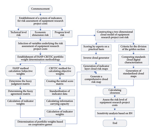
Step 1: establish a cost-risk indicator system for the equipment scientific research project, comprising three primary indicators and twelve secondary indicators.
- ●
Step 2: determine the indicator weights using the FAHP-CRITIC combined weight determination method, grounded in reality and expert opinions.
- ●
Step 3: construct the TDCM to assess the cost risk of the equipment research project. Set the grade standard and create the standard cloud diagram using the improved golden section search method.
- ●
Step 4: input scores for the two primary variables of the secondary indicators into the TDCM to calculate the cloud eigenvalues. Subsequently, combine these eigenvalues with the comprehensive weights of the secondary indicators to calculate the primary indicators’ cloud eigenvalues. These eigenvalues are then combined with their respective weights to generate a complete risk cloud diagram.
- ●
Step 5: calculate the nearness degree of the comprehensive risk cloud diagram relative to the standard cloud diagram and determine the risk level associated with the cost of the equipment research project.
- ●
Step 6: employ BN modeling to perform sensitivity analysis and ascertain the sensitivity level of the risk-assessment indicators.
3. Risk-Assessment Indicator System
The construction of a robust indicator system is crucial in the risk-assessment process. Liang et al. [47] and Yin [48] have developed sophisticated assessment systems in the field of equipment technology risk assessment, which provide valuable references for conducting cost-risk assessments in equipment research projects. Building on the foundational work of the aforementioned studies, this research focuses specifically on cost risk and selects actionable factor indicators. Extensive field research was conducted in scientific research institutes, complemented by a thorough review of relevant literature, exploration of analogous cases, and examination of pertinent regulations and documents concerning the management of national defense scientific research and trial production costs. Expert consultations in relevant fields were also undertaken to validate the scientific and practical applicability of the proposed approach. Consequently, a cost-risk indicator system for equipment research projects has been established, featuring technical, economic, and schedule indicators at the first level and twelve additional indicators at the second level, as depicted in Figure 2.

3.1. Technical Level Risk (R1)
Technical level risks are fundamentally predictive of the advancement required by the project’s technology, which is intrinsically linked to the equipment’s tactical and technical indices. As the tactical technical index increases, the associated challenges in achieving these indices also escalate. At this juncture, it becomes essential to evaluate the mix of old and new technologies, specifically the balance between technological innovation and inheritance. Should the existing technology fall short of meeting the target functionalities, it necessitates the development of new technologies, thereby incurring substantial research and development costs and person-hours dedicated to achieving crucial technological breakthroughs. Conversely, if the existing technology suffices for the target requirements, it is pertinent to assess the degree of alignment with the target technology and whether adjustments in materials or processes are required to integrate into the new project system. It is crucial to recognize the complexity of the technology involved, including whether a combination of multiple technological types is feasible within the system to fulfill the project’s needs. Ensuring technical coordination is vital to preclude cost escalations [49]. Moreover, the technological level of a project may be affected by factors such as the qualifications and credibility of the personnel within the research unit, the working environment, and the organizational structure. These elements can influence the total project cost, inclusive of considerations for equipment wear and tear. Table 1 delineates the criteria for a detailed assessment of technical level risk as elaborated above.
| Secondary indicators | Basis of assessment |
|---|---|
| Technological advancement R11 | Assess the level of technological advancement using technical parameters such as structural technology, precision, accuracy, and other tactical technical indicators to predict the feasibility of achieving the target technology. |
| Technological innovation R12 | Evaluate the potential for breakthroughs in critical technologies based on existing technological reserves and determine if innovation is imperative for the application and development of new technologies. |
| Technological inheritance R13 | Analyze the correlation between the target and existing technologies to ascertain which current technological provisions can support the realization of the target technology. |
| Technical complexity R14 | Evaluate the complexity of the technology in terms of the number of technical disciplines involved, the intricacies of the design principles, and the availability of reference materials. |
| Status of contractors R15 | Assess the adequacy of the initial preparations for technological development, considering factors such as technician qualifications, organizational structure, R&D equipment status, and working environment. |
3.2. Economic Dimension Risk (R2)
Economic dimension risks primarily arise from changes in procurement costs, which are influenced by external factors such as macroeconomic conditions, market sectors, and microeconomic elements. Inflation rates, price increases, and currency devaluations within the national economy directly affect project development and procurement costs. Moreover, shifts in international relations and the restructuring of global dynamics can lead to fluctuations in international exchange rates, which are crucial factors affecting the procurement costs of components that cannot yet be localized. State interventions in project developments, such as tax reductions or exemptions for research units, enhancements in the localization of support equipment, and incentives for outsourcing units to improve service levels, can indirectly influence transaction costs. In addition, the availability of capable contractors within the industry impacts the procurement method. For instance, if there is only one capable contractor, the military may be compelled to engage in single-source procurement. This scenario allows the contractor to exploit cost information asymmetries, potentially skewing costs in their favor and deviating from the actual costs of the equipment research project. The balance of supply and demand within the market determines pricing. When military demand exceeds what the research unit can normally supply, the military finds itself disadvantaged in the dynamic interplay between supply and demand, often resulting in higher costs to meet the research unit’s requirements. The detailed risk assessment at the economic level, based on the analysis above, is outlined in Table 2.
| Secondary indicators | Basis of assessment |
|---|---|
| National economic situation R21 | Evaluate projected changes in procurement costs based on the current state of the national economy, including the presence or absence of inflation. |
| International situation R22 | Forecast changes in procurement costs for imported components based on the international political climate and adjustments in exchange rates. |
| Domestic policy orientation R23 | Analyze the impact of domestic policies, including tax policy, price control, and welfare protection on research projects. |
| Industry environment R24 | Assess how the competitive monopoly relationship and industry-specific policies within the industry environment affect procurement costs. |
| Product supply and demand R25 | Examine changes in procurement costs as influenced by the supply-demand dynamics between suppliers and the demand side over a specified period. |
3.3. Progress Level Risk (R3)
Progress level risk pertains to the uncertainty that the project may not advance as planned, according to either the overall project schedule or individual subproject timelines. Insufficient initial planning of one subsystem’s schedule can adversely affect the development of interconnected subsystems, leading to widespread project disruptions. Effective coordination between the schedules of these subsystems and the overarching project timeline is essential. Only through the realization of a well-configured schedule can an optimal solution be achieved. Delays or interruptions in the project can trigger a cascade of increased costs, including additional employee compensation, enhanced operation of production equipment, liquidated damages, and other consequential expenses. The detailed foundation for assessing progress level risk is illustrated in Table 3.
| Secondary indicators | Basis of assessment |
|---|---|
| Subsystem progress R31 | Assess the reasonableness of each independent subsystem’s schedule based on the network plan diagram. |
| Overall project progress R32 | Evaluate the alignment of the subsystem schedules with the overall project timeline using the network plan diagram. |
Cost risk is associated with the financial expenditures of equipment development projects. The intricacy of the equipment and the unpredictability of both internal and external conditions heighten the risk involved in developing equipment research projects, which in turn impacts the overall cost of delivery. To evaluate the likelihood of cost overruns in these projects, we have selected the probability of occurrence and the degree of impact as variables. A thorough assessment incorporating both dimensions provides a more comprehensive understanding of potential cost risks.
4. Risk-Assessment Model
4.1. FAHP-CRITIC Combined Weight
4.1.1. FAHP Method
-
Step 1: generation of fuzzy pairwise comparison matrices
-
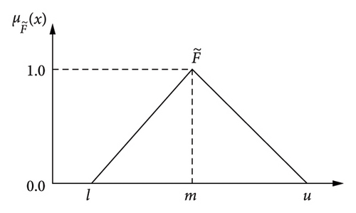
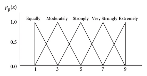
Fuzzy pairwise comparison matrices were constructed at each hierarchical level using precise data collected from experts, who utilized a well-defined fuzzy linguistic scale, as depicted in Table 4. Subsequently, the extent analysis method was applied to compute priority weights using synthetic extent values. The assessment matrix for the fuzzy criteria was formulated by comparing various attributes linked to the overall objective. The correspondence between the TFNs and linguistic terms was established through the adaptation of Saaty’s scale to fuzzy contexts. When a TFN is denoted as , its reciprocal is represented as F−1 = (1/ui, 1/mi, 1/li).
-
In the subsequent step, a fuzzy pairwise comparison matrix was constructed using linguistic terms. Experts applied the nine-point conversion scale to transcribe responses into fuzzy numbers, as illustrated in Table 4.
-
The resultant comparison matrix is formulated as follows:
(2) -
The aggregated fuzzy pairwise comparison matrix, summarized in group decision-making contexts, is represented by the following equation.
(3) -
Here, and k denote the number of experts involved.
-
Step 2: computation of normalized weight values using the geometric mean (GM) method
-
The GM method was utilized to calculate normalized weights for distinct criteria and their relevant subcriteria. The GM method was chosen for its simplicity and effectiveness in determining the principal eigenvalue, thereby minimizing judgment inconsistencies. The procedure commenced with the calculation of the geometric mean for each row of the fuzzy comparison matrix, as outlined in the following equation.
(4) -
Subsequently, the normalized weights for the j th row of the crisp comparison matrix were determined as detailed in the following equation.
(5) -
Here, represents the geometric mean of the fuzzy comparison values, and symbolizes the criterion weights.
-
Step 3: consistency check
-
The consistency ratio (CR) with respect to each pairwise comparison matrix was utilized to control the outcomes of the AHP, requiring a value less than 0.1 for the matrix to be considered consistent. Consistency of a crisp comparison matrix ensures the consistency of the fuzzy pairwise comparison matrix. The consistency index (CI) and CR related to a comparison matrix are described as follows:
(6) -
where λmax is the largest eigenvalue, n is the matrix size, and the standard Random Index (RI) value is obtained using the matrix order.
-
Step 4: defuzzification of the fuzzy weights
-
The Center of Area (COA) method was utilized to defuzzify the weights, which were expressed as fuzzy numbers. This process is encapsulated in the following equation.
(7) -
Step 5: normalization of the crisp weights
-
The crisp criteria weights were determined by normalizing the obtained crisp values. Finally, the subjective weight of the i th evaluation indicator is calculated as follows.
(8)
| Crisp scale | Linguistic terms | TFS scale | Reciprocal TFN scale |
|---|---|---|---|
| 1 | Equally preferred | (1, 1, 1) | (1/1, 1/1, 1/1) |
| 2 | Equally to moderately preferred | (1, 2, 3) | (1/3, 1/2, 1/1) |
| 3 | Moderately preferred | (2, 3, 4) | (1/4, 1/3, 1/2) |
| 4 | Moderately to strongly preferred | (3, 4, 5) | (1/5, 1/4, 1/3) |
| 5 | Strongly preferred | (4, 5, 6) | (1/6, 1/5, 1/4) |
| 6 | Strongly to very strongly preferred | (5, 6, 7) | (1/7, 1/6, 1/5) |
| 7 | Very strongly preferred | (6, 7, 8) | (1/8, 1/7, 1/6) |
| 8 | Very strongly to extremely preferred | (7, 8, 9) | (1/9, 1/8, 1/7) |
| 9 | Extremely preferred | (8, 9, 9) | (1/9, 1/9, 1/8) |
4.1.2. CRITIC Method
-
Step 1: establishment of the initial scoring matrix
-
Assume the scoring matrix includes n objects to be assessed across m assessment indicators. The initial scoring matrix, C, is formulated as shown in the following equation.
(9) -
Step 2: dimensionless processing of indicators
-
The CRITIC method employs both forward and reverse processing to achieve dimensionless indicators, as depicted in equations (10) and (11).
-
Positive indicators:
(10) -
Negative indicators:
(11) -
Step 3: calculation of indicator variability and conflict
-
The variability of an indicator is primarily determined by computing the standard deviation, Sj, using equation (12). A higher Sj value suggests that the indicator conveys more information and is thus deemed more significant. To assess indicator conflict, the Rj value is calculated using equation (13). A lower Rj value indicates a higher degree of information redundancy among indicators, reducing their relative importance.
(12)(13) -
Here, rij represents the correlation coefficient between evaluation indicators i and j.
-
Step 4: calculation of information volume and indicator weight
-
The volume of information an indicator holds is quantified by calculating the standard deviation Zj as per equation (14). A higher Zj value denotes greater significance, which translates into a larger weight for the indicator.
(14) -
Subsequently, the objective weight of the j th evaluation indicator is determined as shown in the following equation.
(15)
4.1.3. Combined Weighting
-
Step 1: linear combination of weights
-
The weight vectors obtained from the FAHP method, , and the CRITIC method, , are linearly combined to form a new vector of indicator weights w = (w1, w2, ⋯, wm) as shown in the following equation.
(16) -
where α1 and α2 are combination coefficients.
-
Step 2: optimization of weight coefficients
-
The coefficients α1 and α2 are optimized using principles from the coalitional game theory. The optimization aims to minimize the deviation of the combined weights w from both w′ and w″. The objective function for this optimization is presented in the following equation.
(17) -
Utilizing matrix differentiation properties, equation (16) is reformulated to solve a system of linear equations, as detailed in the following equation.
(18) -
which yields the optimal solutions for the coefficients and , subject to .
-
Step 3: determination of portfolio weights
-
The final combined weights, , are derived by normalizing the optimal combination coefficients.
(19)
4.2. TDCM Based on Combinatorial Weights
-
Step 1: two-dimensional average cloud model
-
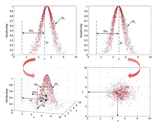
Consider F as a two-dimensional random function adhering to a normal distribution, where Ex and Ey denote the expected values of the two underlying variables and Enx and Eny their respective standard deviations. A model comprising cloud droplets dr op(xi, yi, μi) that satisfies the following equation is defined as a two-dimensional average cloud model:
(20) -
Here, the variables (xi, yi) represent the coordinates of the cloud droplets, while (Pxi, Pyi) denote the conditional coordinates of these droplets. The terms Hex and Hey indicate the hyperentropy, and μi the degree of membership.
-
Step 2: two-dimensional integrated risk cloud
-
To maintain consistency in the evaluation, experts are requested to assess indicators using a 10-point scale based on predefined criteria, which include the likelihood and severity of cost overruns, and the precision of the scoring set at 0.1. The ratings for the probability and impact of cost overruns for each risk indicator are used to form a cloud droplet within the two-dimensional composite risk cloud, which includes separate clouds for risk probability and risk consequence. The numerical properties of this two-dimensional cloud are computed using equation (21) and the MATLAB inverse cloud generator.
(21) -
Equation (21) incorporates the sample expectation Ex, entropy En, hyperentropy He, the k th expert scoring value xk, sample variance S2, and the number of experts q.
-
Initially, the cloud digital feature matrix for the secondary assessment indicators is determined. This matrix is then combined with the corresponding weight vector matrix to compute the cloud digital features for the primary assessment indicators. The synthesis of these features and their weight vector matrix results in the two-dimensional comprehensive risk cloud digital features.
(22) -
where x′En′, and He′ symbolize the expectation, entropy, and hyperentropy of the upper-level indicators, respectively.
-
Step 3: two-dimensional standard cloud
-
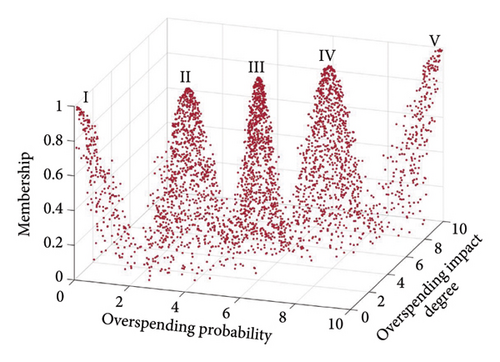
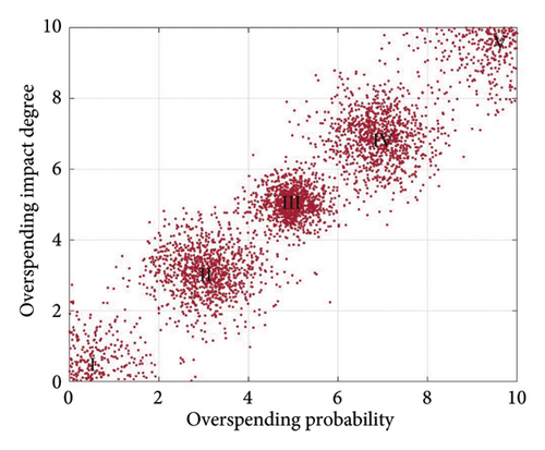
To enhance the clarity of the scoring results, the risk levels associated with the cost of equipment research projects are divided into five defined intervals: minimal risk (I), low risk (II), medium risk (III), high risk (IV), and very high risk (V). These risk categories are delineated by the upper and lower boundary values and , respectively. The classification into these intervals is facilitated by the improved golden section search method, which is adapted to reflect expert scoring preferences [51].
(23)(24)(25) -
Equations (23) through (25) detail the standard cloud’s expectation, entropy, and hyperentropy values. Specifically, Ex0, En0, and He0 denote the central values, while Ex0−1, Ex0−2, En0−1, En0−2, He0−1, and He0−2 represent the values on the left side of the center. Conversely, Ex0+1, Ex0+2, En0+1, En0+2, He0+1, and He0+2 indicate the values on the right side.
-
Given the domain of [0, 10] and a He0 value of 0.1, the specific values for the two-dimensional standard cloud were calculated using equations (23)–(25) and are presented in Table 5.
-
Step 4: risk level cloud map
-
The eigenvalues of the two-dimensional composite risk cloud and the standard cloud are input into the MATLAB forward cloud generator to produce the corresponding cloud graph. The risk level is determined by comparing the proximity of the cloud feature expectation value to the highest point of the cloud map projected in the corresponding coordinate region. The equipment research project cost-risk assessment standard cloud map is depicted in Figure 6.
-
Step 5: calculation of the nearness degree
-
To enhance the precision in determining risk levels, the degree of nearness is employed to measure the congruence between the comprehensive risk cloud map and the standard cloud map. A greater nearness degree value indicates a closer alignment between the comprehensive risk cloud and the corresponding standard cloud level [52].
(26) -
In Equation (26), N denotes the nearness degree, while Ex and Ey represent the expected values of the two base variables of the composite risk cloud. and are the expected values of the two base variables of the standard cloud, respectively.
4.3. Sensitivity Analysis of BNs
-
Step 1: establishment of network structure
-
Given that both the risk-assessment indicator system and the BN are predicated on causal logic relationships, the indicators within the system can act as nodes in constructing the BN. Moreover, as the indicators of the risk-assessment index system are independent, there is no necessity to address the structural learning challenge in the construction of the BN structure. This method prevents the overfitting of both network structure and data that might, otherwise, occur if the construction relied solely on empirical data.
-
Step 2: defining node states
-
Each node possesses two states: State 1, indicating the presence of risk, and State 0, indicating its absence, with a value domain ranging from 0 to 1. In State 1, a value of 0 signifies no risk, 1 signifies a definite risk, and values between 0 and 1 indicate varying probabilities of risk, with higher values correlating with higher risk levels. Conversely, the values for State 0, also within the [0,1] domain, represent the inverse risk implications of State 1.
-
Step 3: sensitivity analysis
-
The parameters for each indicator’s risk level are set according to the TDCM with values of 0.1, 0.3, 0.5, 0.7, and 0.9 for risk Levels I through V, respectively, for State 1. The strength of interrelationships between nodes is quantified through conditional probabilities. Nodes lacking parental nodes are assigned prior probabilities. The parameters for State 0 are defined inversely. The following equations facilitate the sensitivity analysis:
(27)(28) -
Here, SN denotes the selected node, TN the target node, and P(TN) the a priori probability of the target node. The probabilities of the target node under the conditions of SN at its minimum and maximum states SNmin and SNmax are represented by P(TN|SNmin) and P(TN|SNmax), respectively. The metrics of importance for node SN are indicated by Imin(SN) and Imax(SN).
| Scale | Description of the cost-risk level | Description of the probability of overrun | Description of the impact of cost overruns | (Ex0, En0, He0) |
|---|---|---|---|---|
| I | Minimal risk | Minimal probability | Minimal | (0, 1.030, 0.2618) |
| II | Low risk | Small probability | Small | (3.09, 0.6367, 0.1618) |
| III | Medium risk | Medium probability | Medium | (5, 0.3935, 0.1) |
| IV | High risk | High probability | Large | (6.91, 0.6367, 0.1618) |
| V | Very high risk | Very high probability | Extremely large | (10, 1.030, 0.2618) |
5. Case Studies and Discussion
5.1. Project Overview
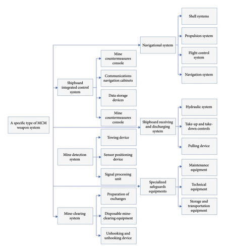
Naval mines represent a prevalent method of covert maritime warfare, posing significant threats to both naval and civilian maritime navigation. The development of a new mine countermeasures (MCMs) weapon system is crucial for accurately identifying, tracking, and neutralizing naval mines, thereby enhancing the naval combat capabilities. This advancement is instrumental in protecting the safety of coastlines and port facilities, and by extension, ensuring the prosperity and stability of sea transportation channels. The development of an MCM weapon system is a multifaceted scientific endeavor that spans multiple technical domains and necessitates substantial resource investment. It is fraught with uncertainties and risks. For example, the creation of a specific MCM weapon system comprises six subsystems, each further divisible into three to six smaller subsystems, as illustrated in Figure 7. This complexity underscores the practical significance and exemplarity of conducting cost-risk assessments for such systems, providing valuable insights for other similar equipment development projects.
5.2. Project Data Collection
In accordance with the aforementioned system of assessment indicators, data were obtained through questionnaires. These questionnaires were anonymous and targeted professionals who were either deeply involved in or highly familiar with the development of MCM weapon systems. Distribution occurred via the Internet and mail, reaching experts and scholars specializing in risk assessment of equipment costs, scientific researchers involved in the development of MCM weapon systems, and operators of these systems. Participants were invited to evaluate the weighting factors, the probability of over-expenditure, and the impact of overexpenditure on each of the 12 secondary indicators. The questionnaire was designed in line with the predefined assessment indicators and included explanatory notes on the relevant indicators to guide the respondents. Scoring was required on a scale from 1 to 10, with 1 representing the least favorable outcome and 10 the most favorable. A total of 56 questionnaires were distributed, of which 47 were returned. Of these returns, 45 were deemed valid for analysis.
5.3. Calculating Index Weight
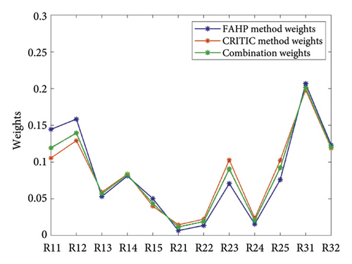
Using the FAHP-CRITIC combined weighting method, the collected weight coefficient data were input into equations (1)–(19). The resultant weights for all the indicators are displayed in Tables 6 and 7, with the distribution of weights for the secondary indicators depicted in Figure 8.
| Primary indicators | Weights | Secondary indicators | Weights | ||||
|---|---|---|---|---|---|---|---|
| FAHP method | CRITIC method | Combined method | FAHP method | CRITIC method | Combined method | ||
| R1 | 0.4874 | 0.4174 | 0.4422 | R11 | 0.1445 | 0.1055 | 0.1193 |
| R12 | 0.1585 | 0.1292 | 0.1396 | ||||
| R13 | 0.0531 | 0.0590 | 0.0569 | ||||
| R14 | 0.0810 | 0.0837 | 0.0828 | ||||
| R15 | 0.0503 | 0.0400 | 0.0436 | ||||
| R2 | 0.1828 | 0.2657 | 0.2340 | R21 | 0.0068 | 0.0146 | 0.0116 |
| R22 | 0.0138 | 0.0222 | 0.0190 | ||||
| R23 | 0.0707 | 0.1029 | 0.0905 | ||||
| R24 | 0.0155 | 0.0235 | 0.0204 | ||||
| R25 | 0.0760 | 0.1025 | 0.0923 | ||||
| R3 | 0.3298 | 0.3169 | 0.3218 | R31 | 0.2067 | 0.1983 | 0.2015 |
| R32 | 0.1231 | 0.1186 | 0.1203 | ||||
| Primary indicators | Weights | Secondary indicators | Weights | ||||
|---|---|---|---|---|---|---|---|
| FAHP method | CRITIC method | Combined method | FAHP method | CRITIC method | Combined method | ||
| R1 | 0.3171 | 0.3407 | 0.3313 | R11 | 0.0673 | 0.0699 | 0.0688 |
| R12 | 0.0971 | 0.1059 | 0.1024 | ||||
| R13 | 0.0310 | 0.0363 | 0.0342 | ||||
| R14 | 0.0818 | 0.0818 | 0.0818 | ||||
| R15 | 0.0399 | 0.0470 | 0.0441 | ||||
| R2 | 0.3969 | 0.3637 | 0.3757 | R21 | 0.0547 | 0.0478 | 0.0503 |
| R22 | 0.0445 | 0.0356 | 0.0388 | ||||
| R23 | 0.0632 | 0.0608 | 0.0617 | ||||
| R24 | 0.0678 | 0.0625 | 0.0644 | ||||
| R25 | 0.1666 | 0.1569 | 0.1604 | ||||
| R3 | 0.2860 | 0.2956 | 0.2920 | R31 | 0.1190 | 0.1217 | 0.1207 |
| R32 | 0.1670 | 0.1739 | 0.1713 | ||||

5.4. Computational Integrated Risk Cloud Digital Characterization
Data concerning the probability and impact of overexpenditure are incorporated into equation (21) to compute the cloud eigenvalues for the primary variables. Table 8 presents both the primary and secondary cloud eigenvalues, calculated by integrating previous results with their respective weights using equation (22). Subsequently, the numerical eigenvalues of the composite risk for the cloud were determined, revealing eigenvalues for the probability of occurrence of overruns for R as (6.855, 0.687, and 0.170) and for the degree of impact of overruns for R as (6.794, 0.676, and 0.162).
| Primary cloud eigenvalues | Secondary cloud eigenvalues | ||||||||
|---|---|---|---|---|---|---|---|---|---|
| Norm | Weights | Probability of overspending | Weights | Degree of impact of overspending | Norm | Weights | Probability of overspending | Weights | Degree of impact of overspending |
| R1 | 0.4422 | (7.636, 0.817, 0.192) | 0.3313 | (8.046, 0.883, 0.206) | R11 | 0.1193 | (7.236, 0.772, 0.163) | 0.0688 | (7.478, 0.698, 0.193) |
| R12 | 0.1396 | (8.115, 0.907, 0.210) | 0.1024 | (8.423, 1.117, 0.213) | |||||
| R13 | 0.0569 | (7.322, 0.683, 0.196) | 0.0342 | (7.884, 0.751, 0.185) | |||||
| R14 | 0.0828 | (8.553, 0.822, 0.182) | 0.0818 | (8.395, 0.992, 0.221) | |||||
| R15 | 0.0436 | (6.731, 0.756, 0.207) | 0.0441 | (8.083, 0.793, 0.198) | |||||
| R2 | 0.2340 | (5.843, 0.587, 0.131) | 0.3757 | (6.012, 0.543, 0.143) | R21 | 0.0116 | (5.432, 0.614, 0.122) | 0.0503 | (5.797, 0.527, 0.151) |
| R22 | 0.0190 | (6.246, 0.505, 0.153) | 0.0388 | (6.223, 0.617, 0.135) | |||||
| R23 | 0.0905 | (6.088, 0.514, 0.115) | 0.0617 | (6.126, 0.506, 0.148) | |||||
| R24 | 0.0204 | (5.607, 0.532, 0.126) | 0.0644 | (5.972, 0.488, 0.155) | |||||
| R25 | 0.0923 | (5.882, 0.557, 0.137) | 0.1604 | (5.923, 0.535, 0.129) | |||||
| R3 | 0.3218 | (6.546, 0.586, 0.171) | 0.2920 | (6.388, 0.613, 0.138) | R31 | 0.2015 | (6.332, 0.608, 0.188) | 0.1207 | (6.435, 0.601, 0.126) |
| R32 | 0.1203 | (6.784, 0.552, 0.156) | 0.1713 | (6.312, 0.622, 0.149) | |||||
5.5. Comprehensive Risk Cloud Mapping
The MATLAB forward cloud generator, utilizing the standard cloud eigenvalues from Table 5 and the comprehensive cloud risk eigenvalues from Table 8, produces comparison diagrams of the common cloud and the total risk cloud, as depicted in Figure 9. These diagrams show that a specific type of MCM weapon system has an integrated risk cloud positioned between the III and IV standard risk clouds but closer to IV. This overlap is particularly evident from the top view, indicating that the cost risk for this MCM weapon system is at a Level IV, which implies a higher risk level.
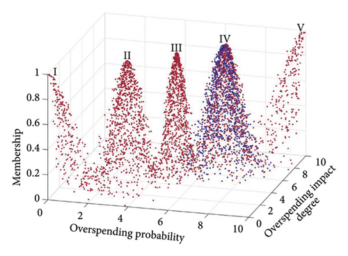
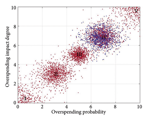
The primary indicator cloud eigenvalues were entered into the MATLAB forward cloud generator to enhance the visualization of specific risks’ impact on the composite risk at the indicator level. This facilitated the creation of comparative maps for each primary indicator cloud, detailed in Figures 10, 11, and 12.
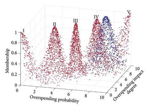
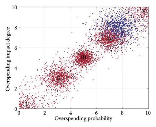
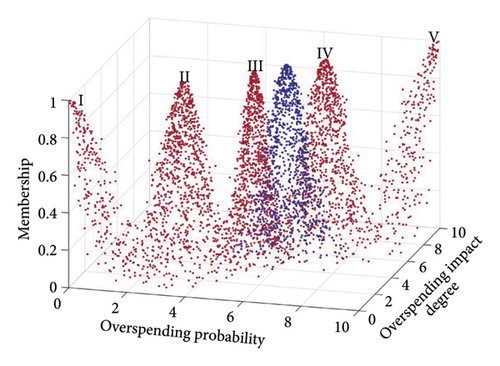
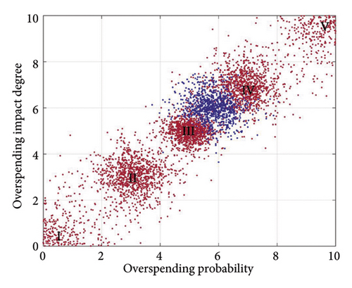
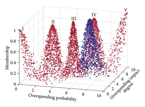
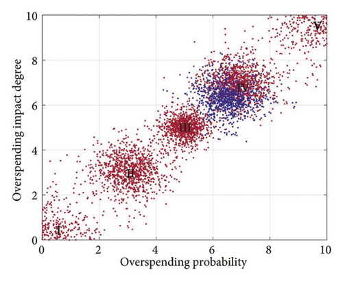
The figures indicate that the technical risk level is situated between Levels IV and V, with IV being more favorable. The economic risk level is positioned between Levels III and IV, while the schedule risk level also falls between Levels III and IV, leaning toward IV. Thus, the highest risk is posed at the technical level, followed by the schedule level, with the economic level presenting the lowest risk.
5.6. Calculating Nearness Degree
Equation (26) is employed to calculate the integrated risk cloud nearness degree and to determine the cost-risk level of a specific MCM weapon system. The nearness degrees of the comprehensive risk cloud to the five standard clouds are expressed as follows: D1 = 0.1037; D2 = 0.1896; D3 = 0.3884; D4 = 7.4536; and D5 = 0.2224. These results rank the nearness degree as D4 > D5 > D3 > D2 > D1, with the highest nearness degree to the IV standard cloud. It has been determined that the cost risk of developing this specific type of MCM weapon system is moderately high, aligning with the risk level indicated by the project’s development institute. Prioritizing cost-risk management during project development is essential, which may involve reducing the development proportion or pausing the project until further prestudy results are available.
5.7. Sensitivity Analysis
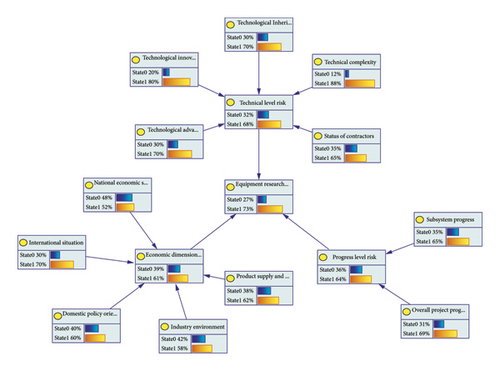
The BN topology was established based on the data from Table 2, with node parameters assigned according to the corresponding indicator’s risk level. Sensitivity analysis was conducted utilizing equations (27) and (28). The structure of the BN for a specific MCM weapon system was illustrated using GeNIe software, as shown in Figure 13.
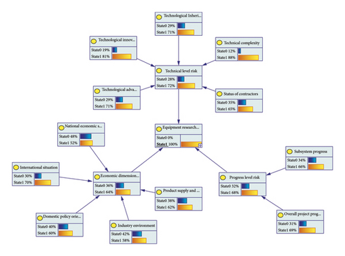
Within this BN model, the “equipment research project cost risk” node was designated as the evidence node, with State 1 set at 100%. Inverse deduction was employed to identify the principal influencing nodes, as depicted in Figure 14. This figure demonstrates that the specific MCM weapon system exhibits a higher risk of increased costs associated with technical complexity (R14), technical inheritance (R13), technological advancement (R11), international situation (R22), and overall project progress (R32), with the probability of these risks exceeding 69%.
Further analysis of the sensitivity results, shown in Figure 15, indicates that the nodes representing technical complexity (R14), technological innovation (R12), technical inheritance (R13), technological advancement (R11), and subsystem progress (R31) exhibit heightened sensitivity to the target node when development cost risks are considered for the same MCM weapon system.
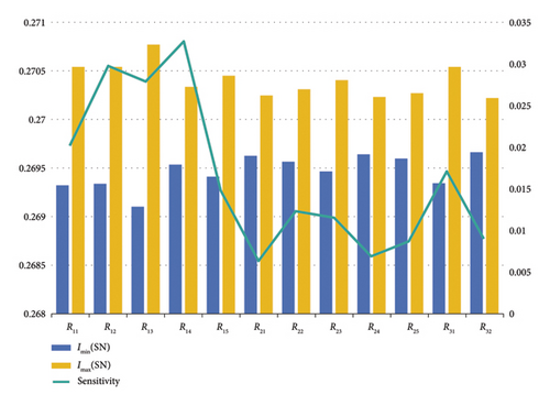
The combination of inverse deduction and sensitivity calculations highlights that technical complexity (R14) exerts the most significant influence on the development costs of the specified MCM weapon system, followed by technical inheritance (R13) and technological advancement (R11). The project development team should prioritize these three areas and implement targeted control measures. It is crucial to leverage the experience gained from existing MCM weapon systems in technical development. Technological innovation should be pursued by fully integrating core technologies, attracting research talents, offering scientific and technological incentives, and fostering technological collaborations. Vigilant management of the project development plan is necessary to avoid undue additional costs due to delays related to technical research or other factors, thereby keeping potential cost risks within a reasonable range.
5.8. Discussion
The FAHP and CRITIC methods are individually utilized to compute the weights of various indicators. By aggregating the cloud eigenvalues of each indicator, integrated cloud eigenvalues R′ and R″ corresponding to these methods are derived. These values are subsequently compared with the integrated cloud eigenvalues R, which are calculated using the combined FAHP-CRITIC weighting method. The expected values of the integrated cloud eigenvalues are determined by inserting them into equation (26) to ascertain the degree of nearness, thereby affirming the efficacy and applicability of the proposed methodology. Due to space constraints, only the cloud feature expectation value is provided as an illustration; detailed results are presented in Tables 9 and 10.
| Comprehensive risk cloud eigenvalues | Primary cloud eigenvalues | ||||||
|---|---|---|---|---|---|---|---|
| Sports event | Probability of overspending | Degree of impact of overspending | Norm | Weights | Probability of overspending | Weights | Degree of impact of overspending |
| R′ | 6.983 | 6.768 | 0.4874 | 7.698 | 0.3171 | 8.120 | |
| 0.1828 | 5.949 | 0.3969 | 5.980 | ||||
| 0.3298 | 6.501 | 0.2860 | 6.363 | ||||
| R″ | 6.868 | 6.821 | 0.4174 | 7.736 | 0.3407 | 8.118 | |
| 0.2657 | 5.943 | 0.3637 | 5.978 | ||||
| 0.3169 | 6.501 | 0.2956 | 6.363 | ||||
| R | 6.855 | 6.794 | R1 | 0.4422 | 7.636 | 0.3313 | 8.046 |
| R2 | 0.2340 | 5.843 | 0.3757 | 6.012 | |||
| R3 | 0.3218 | 6.546 | 0.2920 | 6.388 | |||
| Norm | D1 | D2 | D3 | D4 | D5 | Order of closeness |
|---|---|---|---|---|---|---|
| R′ | 0.1028 | 0.1867 | 0.3764 | 6.262 | 0.2262 | D4 > D3 > D5 > D2 > D1 |
| R″ | 0.1033 | 0.1883 | 0.3833 | 10.1613 | 0.2241 | D4 > D3 > D5 > D2 > D1 |
| R | 0.1037 | 0.1896 | 0.3884 | 7.4536 | 0.2224 | D4 > D3 > D5 > D2 > D1 |
The data in Tables 9 and 10 indicate that the rankings of nearness degree, as obtained by the three distinct methods—FAHP, CRITIC, and the integrated FAHP-CRITIC—are consistent. This consistency underscores the validity and reliability of the FAHP-CRITIC combined weighting approach. Moreover, the integrated FAHP-CRITIC method amalgamates subjective weights derived from the FAHP method with objective weights calculated via the CRITIC method. The resultant cloud eigenvalues and degrees of nearness are more stable compared with those derived from either the FAHP or CRITIC methods alone, further corroborating the practical utility of this approach in the context of complex equipment research projects.
Despite its advantages, the FAHP-CRITIC combined weighting approach exhibited several limitations during the case study: (1) the overall computational process is intricate, necessitating extensive mathematical operations and logical reasoning. (2) The requirements for data modeling and analysis are stringent; incomplete datasets can lead to erroneous assessment outcomes. (3) The absence of standardized cloud numerical feature divisions can result in significant discrepancies in the assessment outcomes for the same issue under different standards.
In response to these challenges, future research should focus on the following areas: (1) simplifying the calculation process of the TDCM by integrating machine learning and artificial intelligence technologies to automate feature extraction and risk assessment, thereby reducing subjectivity and human error and enhancing the efficiency of assessments. (2) Developing methodologies to manage incomplete data, incorporating real-time data for dynamic analysis to ensure that the most current risk information is promptly acquired for ongoing adjustments and updates. (3) Reducing reliance on historical data and promoting the practical implementation of the TDCM to accumulate research experience, establish international consensus through cooperation, and develop a unified standard for cloud numerical feature division to minimize discrepancies and ensure consistency in assessment results.
6. Conclusion
- ●
A comprehensive system of cost-risk assessment indicators has been established, tailored to the nuances of equipment research project development. This involved a thorough review of relevant literature and consultations with experts. The principal factors influencing cost risk were analyzed across three dimensions: technology (R1), economy (R2), and schedule (R3). This analysis facilitated the internal mechanism of indicator selection, culminating in the construction of a risk-assessment framework comprising 12 secondary indicators.
- ●
Design of cost-risk assessment methods. (1) The coalitional game theory was employed to assign combined weights to the FAHP and CRITIC methods, ensuring both subjective and objective weights of the assessment indicators were comprehensively calculated. (2) Implementation of TDCM in cost-risk assessment. By integrating expert scoring on the probability and impact of overspending, cloud eigenvalues are computed. The cost-risk level is then determined comprehensively by comparison with standard cloud eigenvalues. (3) A BN topology was developed based on the intrinsic relationships among the assessment indicators. A sensitivity analysis was designed to identify which indicators are most responsive to changes.
- ●
A specific MCM weapon system was selected as a case study to conduct a cost-risk assessment and to validate both the index system and the assessment methodology. The findings are presented as follows: (1) The calculated nearness degrees for the MCM weapon system were ranked as D4 > D5 > D3 > D2 > D1, indicating a moderately high cost risk. (2) Following the sensitivity analysis, targeted risk-control recommendations were formulated for the three critical nodes: R14, R13, and R11. (3) The validity and feasibility of the cost-risk assessment model were confirmed by comparing the outcomes derived from three distinct methods.
Disclosure
The preprint was posted on ResearchGate under the title “Risk Assessment of Equipment Research Project Costs Based on FAHP-CRITIC Combined Weights for 2D Cloud Models,” Doi number: https://doi.org/10.21203/rs.3.rs-3875285/v1.
Conflicts of Interest
The authors declare no conflicts of interest.
Author Contributions
C.Z. wrote the main text of the manuscript; S.S. provided data support; T.C. and Q.Z. revised it; C.Z. and H.L. performed model simulations and collaborated in the preparation of the figures; J.L. and D.H. helped to improve some of the figures; and all authors reviewed the manuscript.
Funding
The research was supported by the National Social Science Foundation of China under Grant nos. 18BGL287 and 19CGL073.
Acknowledgments
This research was supported by National Social Science Foundation of China under Grant nos. 18BGL287 and 19CGL073.
Open Research
Data Availability Statement
The datasets generated during and/or analyzed during the current study are not publicly available but are available from the corresponding author on reasonable request.


