Volume 2025, Issue 1 5568285

Research Article

Open Access

Optimal Algebras and Novel Solutions of Time-Fractional (2 + 1) − D European Call Option Model

Gimnitz Simon S.

orcid.org/0009-0000-4156-8856

Department of Mathematics , College of Engineering and Technology , SRM Institute of Science and Technology , Kattankulathur , 603203 , Tamil Nadu, India , srmist.edu.in

Search for more papers by this author

B. Bira,

Corresponding Author

B. Bira

[email protected]

orcid.org/0000-0002-7414-8775

Department of Mathematics , College of Engineering and Technology , SRM Institute of Science and Technology , Kattankulathur , 603203 , Tamil Nadu, India , srmist.edu.in

Search for more papers by this author

Sathiyaraj Thambiayya,

Sathiyaraj Thambiayya

orcid.org/0009-0007-4366-6311

Institute of Actuarial Science and Data Analytics , UCSI University , Kuala Lumpur , 56000 , Malaysia , ucsiuniversity.edu.my

Search for more papers by this author

Gimnitz Simon S.,

Gimnitz Simon S.

orcid.org/0009-0000-4156-8856

Department of Mathematics , College of Engineering and Technology , SRM Institute of Science and Technology , Kattankulathur , 603203 , Tamil Nadu, India , srmist.edu.in

Search for more papers by this author

B. Bira,

Corresponding Author

B. Bira

[email protected]

orcid.org/0000-0002-7414-8775

Department of Mathematics , College of Engineering and Technology , SRM Institute of Science and Technology , Kattankulathur , 603203 , Tamil Nadu, India , srmist.edu.in

Search for more papers by this author

Sathiyaraj Thambiayya,

Sathiyaraj Thambiayya

orcid.org/0009-0007-4366-6311

Institute of Actuarial Science and Data Analytics , UCSI University , Kuala Lumpur , 56000 , Malaysia , ucsiuniversity.edu.my

Search for more papers by this author

First published: 08 May 2025

https://doi.org/10.1155/ddns/5568285

Academic Editor: Palanivel M.

Share a link

Email
Wechat
Bluesky

Abstract

In this article, we analyse the time-fractional (2 + 1) − D Black–Scholes model for European call options by employing Lie symmetry analysis. We derive the infinitesimal transformations and classify the optimal systems. Furthermore, under the geometric Brownian motion, we reduced the given model to ordinary differential equation (ODE) with integer order. We have obtained different ODEs for different correlation values. Then, we construct the power series solutions and established its convergence. Furthermore, the reduced ODE is simulated numerically and the solutions are illustrated graphically. Finally, we explicitly find the conserved vectors.

1. Introduction

In the present era, finance and financial economic encompassing balancing risk and return, investment in stocks, managing debt or optimizing corporate capitals, plays vital role. The nature of the financial markets is nonlinear phenomena as it involves volatility, correlation along with much more factors. This nonlinear phenomena can be well described and studied by mathematical models. Differential calculus dealing with derivatives is an efficient process to capture the rate of changes occurring in real life phenomena. For example, the Black–Scholes option pricing equation involving the derivative of option pricing is used for pricing European-style options [1].

This model helps in calculating the theoretical price of options by assuming that the underlying asset (e.g., a stock) has no dividends and that the market is frictionless with a constant risk-free interest rate. An empirical study was also conducted over the Black–Scholes model [2]. Several researchers have contributed to the development of the Black–Scholes model by studying using different techniques such as nonstandard finite difference method for American put option pricing in [3], dynamic calibration by Bayesian methods in [4], with help of orthogonal Gegenbauer polynomials in [5]. Even Lie symmetry has been utilised to Black–Scholes in different forms such as with time-dependent coefficients [6], bifractional under fractional G-Brownian motion [7] and (1 + 1) generalised Black–Scholes in [8].

Recently, many financial experts are introducing the concept of fractional derivative in this field, as it is an effective tool to study nonlocal properties of nonlinear physical phenomena with memory index [9–12]. Hence, in our present work, we consider (2 + 1) − D time-fractional Black–Scholes model to study European call options u(t, x, y) on a basket of two assets:

()

with μ as the fractional order 0 < μ < 1, where α₁ and α₂ are the expected rate of returns, σ₁ and σ₂ are the volatilities, ρ is the correlation between two assets, and k is arbitrary. When μ = 1, model (1) reduces a partial differential equation (PDE), which is studied by the authors in [13]. In a pragmatic point of view, the Black–Scholes model is one of those models where the model performs better as the dimension increases because a portfolio is never based on only one stock. However, the given model with fractional order derivative is new in the literature and significant. For a reader with no prior economics knowledge, we explain this in simple terms. A stock that is an asset is bought in share market by an investor and can be sold upon the choice of the investor. To buy a stock, an investor can call for a price, which is called the strike price. The investor can buy the stock at strike price even if the price goes up after making investor’s call. Optimising the strike price will eventually benefit the investor. In addition, a technique called “hedging” is used to lower the risk of bad price changes in an asset. To protect against possible losses, it means taking a compensating position in a related property or investment. Hedging is often used in the stock market.

On the other hand, it is not an easy task to construct an exact solution for a given fractional differential equation. Lie symmetry analysis is highly effective and simple approach to deal with such fractional PDEs [14–16]. This can be explored in different areas including biological [17], fluid dynamics [18, 19], and geophysical flows [20, 21]. Currently, the study is also advanced by including Nucci reduction, nonclassical solutions [22–25]. A symmetry of an FPDEs is a one-parameter Lie group of transformations that translates one solution to another while keeping the system invariant [26, 27]. Furthermore, the given FPDE may have infinite solutions and one must minimize the search for accurate solutions. Hence, the classification of optimal system of inequivalent subalgebra is needed [28, 29].

We organise this paper as follows: we perform symmetry analysis in Section 2 and we optimise the obtained subalgebras in Section 3. In Section 4, we construct an exact solution using power series, perform numerical simulation, and analyse multiple parameters with the help of graphs. We calculate the conserved vectors in Section 5. Finally, we conclude by a brief conclusion in Section 6.

2. Symmetry Analysis

Riemann–Liouville (R–L) fractional derivative.

The R–L fractional derivative of order μ for the integrable function f(t) is defined as follows:

()

where n ∈ N. In order to derive the symmetry group of transformations of (1), we first consider the one-parameter (ϵ) infinitesimal Lie group of transformations as follows:

()

where τ, η, ν, and φ are the infinitesimals to be determined. The infinitesimal generator corresponding to (1) can be written as follows:

()

Since, model (1) is second-order PDE with fractional derivative, we take the prolongation of (4) as follows:

()

where

()

Applying (5) in (1), one can obtain set of overdetermining equations and which on solving yields

()

The symmetry generators associated with (7) are

()

3. Optimal Algebra

In order to classify the optimal algebras, first, we ensure the commutative and adjoint properties of (8). For that, we consider the Lie bracket as follows:

()

and obtained Table 1.

Table 1. Commutator table.

∗	X₁	X₂	X₃	X₄
X₁	0	0	X₁	0
X₂	0	0	X₂	0
X₃	−X₁	−X₂	0	−X₄
X₄	0	0	X₄	0

Furthermore, considering the following adjoint relation:

()

we obtained Table 2.

Table 2. Adjoint table.

Adj	X₁	X₂	X₃	X₄
X₁	X₁	X₂	X₃	X₄
X₂	X₁	X₂	X₃ − εX₂	X₄
X₃			X₃
X₄	X₁	X₂	X₃ − εX₄	X₄

Using Table 1 and Table 2, we construct invariant function (ψ).

Now, we consider

and

with

()

with

()

Differentiating (11), w.r.t ε at ε = 0, and considering the coefficients of

, we obtain

()

From the above system of equations, one can obtain the invariant function ψ = (f₁, f₂), which implies that the classified subalgebras will be isomorphic to the vector space spanned by X₁ and X₂. Furthermore, from adjoint action, we get ϰ₃ = 0, which implies X₃ itself is an one dimensional optimal algebra. Hence, we can span 2-dimensional algebra along with X₃. Thus, we find 〈X₁ ± X₂, X₃〉 as the optimal subalgebras.

4. Exact Solution

Under the geometric Brownian motion, α₁ = α₂ = α and σ₁ = σ₂ = σ, we consider the following three cases.

Case 1. For ρ = 1.

When ρ = 1, one can get the optimal algebra as 〈X₁ − X₂, X₃〉. The method of characteristics corresponding to 〈X₁ − X₂〉 is

()

The few invariant solutions of (14) are l₁ = t, l₂ = u, l₃ = x + y. Now, rewriting the algebra X₃ with the help of new invariants, we get the characteristics as follows:

()

Upon simplifying, we obtain the similarity variables as follows:

()

In R–L sense, we get

()

Using

and (16) in (1), we get the reduced FODE as follows:

()

where the left-hand side Erdelyi–Kober fractional integral operator

is defined as follows [20]:

()

Furthermore, taking the equivalent form of

as follows [30]:

()

we reduce (18) to an ODE with integer order given as follows:

()

where A = ((1 + μ/2)/(2 + (3μ)/2)) and B = (1/(2 + (3μ)/2)).

Next, we consider

()

and applying in (21), which yields the recurrence relation of coefficients given as follows:

()

Thus, the solution of (21) is obtained as follows:

()

Hence, the solution of (1) can be written as follows:

()

4.1. Convergence Analysis of (25)

We establish that (25) is convergent by comparison. For that, we consider a series

()

First, we shall prove (26) is majorant of (22) and then (26) has positive finite radius of convergence.

From the relation of coefficients of (25), we have,

()

Thus, we have |a_n| ≤ s_n, implying (26) is majorant. To verify the signum and magnitude of radius, we rewrite

()

Taking the fractional increment into account, we define

()

Clearly, from the above equation, we see G(0, v₀) = 0 and G^′(0, v₀) ≠ 0 proving that V(ξ) is convergent in a neighbourhood of the point (0, s₀) using implicit function theorem.

Hence, we can conclude that (25) is convergent.

Case: 2. For ρ = −1.

When ρ = −1, we have the optimal algebra 〈X₁ + X₂, X₃〉 and following the similar procedure as in Case 1, we get the exact solution for (1) as follows:

()

Similarly, if we consider (26), we can prove the convergence of (30).

Case 3. For ρ = 0.

When ρ = 0, with the help of ansatz u = f(t), the governing equation gets simplified into with a trivial solution given as u = c₁t^μ−1.

4.2. Numerical Simulation

For the numerical simulation, we consider a situation when the stock price is translated to the initial state at the opening bell, that is, u(x, y, 0) = 0, with invariant condition U(ξ) = 0 in (21) and discuss the behaviour of option price using the finite collocation method.

5. Results and Discussion

•
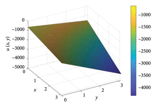
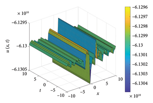
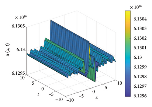
From Figure 1, it is observed that at a fixed time, for a basket of two positively correlated assets, the price of call options declines linearly. Furthermore, when the stock price is fixed for one asset and as time progresses, the option pricing oscillates giving the rogue waves and dark soliton type solution, which is presented in Figure 2.
•
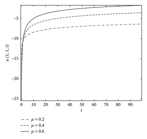
If the stock price of basket of assets is fixed for a long time, it is trivial that it does not affect the decision of buyers. Therefore, the option call pricing decays significantly. Furthermore, as the fractional order μ increases, the rate of call option pricing attains at-the-money state faster, which is noticed in Figure 3.
•
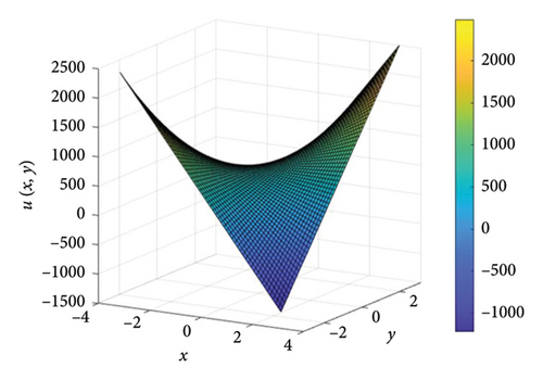
If the two assets are negatively correlated, for a given fixed time, then the price of call options are inversely proportional to each other and it is observed in Figure 4. Furthermore, it is noticed that when the stock price is fixed for one asset, then the option pricing gives rogue waves and bright soliton as time progresses, which is shown in Figure 5.
•
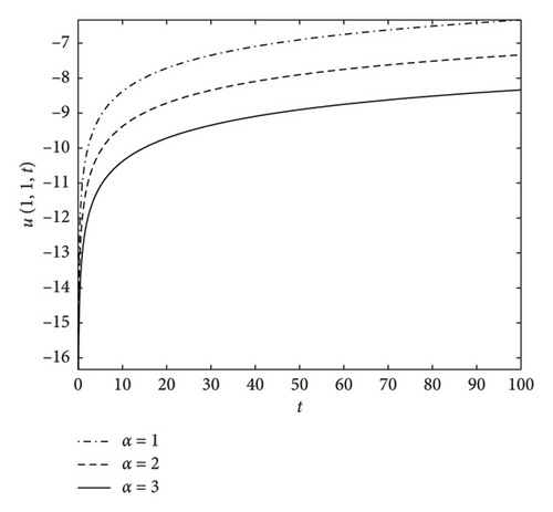
In Figure 6, we fluctuate the expected rate of return (α) and observe its influence on option call pricing. We notice that, as the expected rate of return increases, investors tend to hold the stocks and as a result, the option call price gets lowered. This movement is very gradual.
•
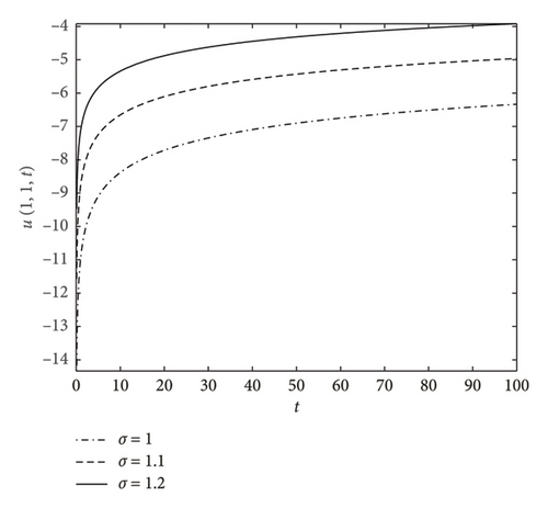
Furthermore, increase in volatility rate (σ) attracts more traders; as a result, the option call pricing increases. This movement is very sensitive, which is illustrated in Figure 7.
•
Figure 8 clearly indicates that the option call pricing profile is decreasing in an extended run, showing that the option call pricing becomes stable. Furthermore, the critical point which diminishes the initial peak is crucial for selling, that is, exiting.

6. Conservation Laws

The conservation laws provide physical interpretation of the model and are due to [31].

Details are in the caption following the image — **Figure 1**
Open in figure viewer PowerPoint

Dynamics of (25) for fixed t.

The formal Lagrangian for (1) is considered as follows:

()

where

is the new dependent variable. The adjoint equation for the above formal Lagrangian is given as follows [32]:

()

with the Euler–Lagrangian operator defined as follows:

()

where

is an adjoint operator of

Subsequently, the R–L fractional differential operator is given as follows:

()

and

is the right-sided Caputo operator.

Also, the conservation laws for (1) are given as follows:

()

where T^x = T^x(x, y, t, u, …), T^y = T^y(x, y, t, u, …), and T^t = T^t(x, y, t, u, …) are the conserved vectors found from the following:

()

Similarly, one can obtain for T^y with ^uW_j = φ_j − (η_ju_x + ν_ju_y + τ_ju_t). Also, a = 1, 2, 3, 4 are the number of symmetries obtained and the integral

is given as follows:

()

For X₁:

We have the Lie characteristic as follows:

()

which yields

()

For X₂:

We have the Lie characteristic as follows:

()

For X₃:

We have the Lie characteristic as follows:

()

7. Conclusion

In this work, we have analysed a (2 + 1) -D time-fractional Black–Scholes equation through the lens of Lie symmetry. Using the Lie group, we have reduced our governing equation into an ODE with integer order and, successively, we have constructed some power series solutions. We established the convergence of power series solutions and also simulated the reduced ODE numerically. Furthermore, we have obtained the conserved vectors to delve into physical properties. From our study, we conclude that hedging is a smart stock market practice; if the expected rate of return is high, investors tend to hold it for long term, resulting in a stable price. Thus, the stock trading movement becomes slow and increase in fractional order μ, making the stock price attain “at the money” state quickly.

Conflicts of Interest

The authors declare no conflicts of interest.

Funding

The authors did not receive any specific funding for this work.

Open Research

Data Availability Statement

No new data were generated in this work.

References

1 Black F. and Scholes M., The Pricing of Options and Corporate Liabilities, Journal of Political Economy. (1973) 81, no. 3, 637–654, https://doi.org/10.1086/260062.
10.1086/260062
Web of Science® Google Scholar
2 Lauterbach B. and Schultz P., Pricing Warrants: an Empirical Study of the Black-Scholes Model and its Alternatives, The Journal of Finance. (1990) 45, no. 4, 1181–1209, https://doi.org/10.1111/j.1540-6261.1990.tb02432.x, 2-s2.0-84977731800.
10.1111/j.1540-6261.1990.tb02432.x
Web of Science® Google Scholar
3 Shahmorad S., Kalantari R., and Assadzadeh A., Numerical Solution of Fractional Black-Scholes Model of American Put Option Pricing via a Nonstandard Finite Difference Method: Stability and Convergent Analysis, Mathematical Methods in the Applied Sciences. (2021) 44, no. 4, 2790–2805, https://doi.org/10.1002/mma.5913.
10.1002/mma.5913
Google Scholar
4 Mulenga N. and Fu Y., Dynamic Calibration Based on the Black-Scholes Option Pricing Model by Bayesian Method, IEEE Access. (2024) 12, 119314–119326, https://doi.org/10.1109/access.2024.3450602.
10.1109/ACCESS.2024.3450602
Google Scholar
5 Aghdam Y., Mesgarani H., Amin A., and Gómez-Aguilar J. F., An Efficient Numerical Scheme to Approach the Time Fractional Black–Scholes Model Using Orthogonal Gegenbauer Polynomials, Computational Economics. (2024) 64, no. 1, 211–224, https://doi.org/10.1007/s10614-023-10444-w.
10.1007/s10614-023-10444-w
Web of Science® Google Scholar
6 Yu J. and Feng Y., Group Classification of Time Fractional Black-Scholes Equation with Time-dependent Coefficients, Fractional Calculus and Applied Analysis. (2024) 27, no. 5, 2335–2358, https://doi.org/10.1007/s13540-024-00339-4.
10.1007/s13540-024-00339-4
Google Scholar
7 Yu J., Feng Y., and Wang X., Lie Symmetry, Exact Solutions and Conservation Laws of Bi-fractional Black–Scholes Equation Derived by the Fractional G-Brownian Motion, International Journal of Financial Engineering. (2024) 11, no. 01, https://doi.org/10.1142/s2424786323500378.
10.1142/S2424786323500378
Web of Science® Google Scholar
8 Yu J., Feng Y., and Wang X., Lie Symmetry Analysis and Exact Solutions of Time Fractional Black–Scholes Equation, International Journal of Financial Engineering. (2022) 09, no. 04, https://doi.org/10.1142/s2424786322500232.
10.1142/S2424786322500232
Google Scholar
9 Mandal H., Bira B., and Zeidan D., Optimal Algebra and Power Series Solution of Fractional Black-Scholes Pricing Model, Soft Computing. (2021) 25, no. 8, 6075–6082, https://doi.org/10.1007/s00500-021-05600-z.
10.1007/s00500-021-05600-z
Google Scholar
10 Padmaja N., Designing Sampled Data Controller for Time-Delayed Fractional-Order Neural Networks via a New Functional Approach, European Physical Journal: Special Topics. (2024) 1-12, https://doi.org/10.1140/epjs/s11734-024-01261-9.
10.1140/epjs/s11734-024-01261-9
Google Scholar
11 Saravanakumar S. and Balasubramaniam P., Non-instantaneous Impulsive Hilfer Fractional Stochastic Differential Equations Driven by Fractional Brownian Motion, Stochastic Analysis and Applications. (2021) 39, no. 3, 549–566, https://doi.org/10.1080/07362994.2020.1815545.
10.1080/07362994.2020.1815545
Web of Science® Google Scholar
12 Rehman Z. U., Boulaaras S., Jan R., Ahmad I., and Bahramand S., Computational Analysis of Financial System through Non-integer Derivative, Journal of Computational Science. (2024) 75, https://doi.org/10.1016/j.jocs.2023.102204.
10.1016/j.jocs.2023.102204
Google Scholar
13 Cimpoiasu R. and Constantinescu R., New Symmetries and Particular Solutions for 2D Black-Scholes Model, Proceedings of the 7th Mathematical Physics Meeting: Summer School and Conference on Modern Mathematical Physics, 2012, Belgrade, Serbia, 9–12.
Google Scholar
14 Tayyan B. and Sakka A., Lie Symmetry Analysis of Some Conformable Fractional Partial Differential Equations, Arabian Journal Of Mathematics. (2020) 9, no. 1, 201–212, https://doi.org/10.1007/s40065-018-0230-8.
10.1007/s40065-018-0230-8
Web of Science® Google Scholar
15 Yu J. and Feng Y., Lie Symmetry Analysis, Power Series Solutions and Conservation Laws of (2+ 1)-Dimensional Time Fractional Modified Bogoyavlenskii–Schiff Equations, Journal of Nonlinear Mathematical Physics. (2024) 31, no. 1, 27–23, https://doi.org/10.1007/s44198-024-00195-z.
10.1007/s44198-024-00195-z
Google Scholar
16 Yu J. and Feng Y., Symmetry Analysis, Optimal System, Conservation Laws and Exact Solutions of Time-Fractional Diffusion-type Equation, International Journal of Geometric Methods in Modern Physics. (2024) 22, no. 03, https://doi.org/10.1142/s0219887824502864.
10.1142/s0219887824502864
Google Scholar
17 San S. and Yaşar E., On the Lie Symmetry Analysis, Analytic Series Solutions, and Conservation Laws of the Time Fractional Belousov–Zhabotinskii System, Nonlinear Dynamics. (2022) 109, no. 4, 2997–3008, https://doi.org/10.1007/s11071-022-07549-6.
10.1007/s11071-022-07549-6
Google Scholar
18 Yu J. and Feng Y., On the Generalized Time Fractional Reaction–Diffusion Equation: Lie Symmetries, Exact Solutions and Conservation Laws, Chaos, Solitons & Fractals. (2024) 182, https://doi.org/10.1016/j.chaos.2024.114855.
10.1016/j.chaos.2024.114855
Google Scholar
19 Rashidi S. and Hejazi S., Analyzing Lie Symmetry and Constructing Conservation Laws for Time-Fractional Benny–Lin Equation, International Journal of Geometric Methods in Modern Physics. (2017) 14, no. 12, https://doi.org/10.1142/s0219887817501705, 2-s2.0-85028304941.
10.1142/S0219887817501705
Google Scholar
20 Liu J., Zhang Y., and Wang J., Investigation of the Time Fractional Generalized (2+ 1)-dimensional Zakharov–Kuznetsov Equation with Single-Power Law Nonlinearity, Fractals. (2023) 31, no. 05, https://doi.org/10.1142/s0218348x23500330.
10.1142/S0218348X23500330
Google Scholar
21 Yu J. and Feng Y., Lie Symmetries, Exact Solutions and Conservation Laws of Time Fractional Boussinesq–Burgers System in Ocean Waves, Communications in Theoretical Physics. (2024) 76, no. 12, https://doi.org/10.1088/1572-9494/ad71ab.
10.1088/1572-9494/ad71ab
Google Scholar
22 Gülşen S., Yao S. W., and Inc M., Lie Symmetry Analysis, Conservation Laws, Power Series Solutions, and Convergence Analysis of Time Fractional Generalized Drinfeld-Sokolov Systems, Symmetry. (2021) 13, no. 5, https://doi.org/10.3390/sym13050874.
10.3390/sym13050874
Google Scholar
23 Youssoufa M., Gulsen S., Hashemi M. S., Rezapour S., and Inc M., Novel Exact Solutions to the Perturbed Gerdjikov–Ivanov Equation, Optical and Quantum Electronics. (2024) 56, no. 7.
10.1007/s11082-024-07166-0
Google Scholar
24 Gulsen S., Hashemi M. S., Alhefthi R., Inc M., and Bicer H., Nonclassical Symmetry Analysis and Heir-Equations of Forced Burger Equation with Time Variable Coefficients, Computational and Applied Mathematics. (2023) 42, no. 5, https://doi.org/10.1007/s40314-023-02358-y.
10.1007/s40314-023-02358-y
Google Scholar
25 Yao S. W., Gulsen S., Hashemi M. S., Inc M., and Bicer H., Periodic Hunter–Saxton Equation Parametrized by the Speed of the Galilean Frame: Its New Solutions, Nucci’s Reduction, First Integrals and Lie Symmetry Reduction, Results in Physics. (2023) 47, https://doi.org/10.1016/j.rinp.2023.106370.
10.1016/j.rinp.2023.106370
Google Scholar
26 Bluman G. and Kumei S., Symmetries and Differential Equations, 2013, Springer Science & Business Media.
Google Scholar
27 Olver P., Equivalence, Invariants and Symmetry, 1995, Cambridge University Press.
10.1017/CBO9780511609565
Google Scholar
28 Ovsiannikov L., Group Analysis of Differential Equations, 2014, Academic Press.
Google Scholar
29 Olver P., Applications of Lie Groups to Differential Equations, 1993, Springer Science & Business Media.
10.1007/978-1-4612-4350-2
Google Scholar
30 Costa F., Marao J., Soares J., and de Oliveira E. C., Similarity Solution to Fractional Nonlinear Space-Time Diffusion-Wave Equation, Journal of Mathematical Physics. (2015) 56, no. 3, https://doi.org/10.1063/1.4915293, 2-s2.0-85009943143.
10.1063/1.4915293
PubMed Google Scholar
31 Ibragimov N. H., A New Conservation Theorem, Journal of Mathematical Analysis and Applications. (2007) 333, no. 1, 311–328, https://doi.org/10.1016/j.jmaa.2006.10.078, 2-s2.0-34248188617.
10.1016/j.jmaa.2006.10.078
Web of Science® Google Scholar
32 Shagolshem S., Bira B., and Nagaraja K., Exact Solutions, Conservation Laws, and Shock Wave Propagation of Two-Lanes Traffic Flow Model via Lie Symmetry, Physics of Fluids. (2024) 36, no. 8, https://doi.org/10.1063/5.0222213.
10.1063/5.0222213
Google Scholar

All articles

Optimal Algebras and Novel Solutions of Time-Fractional (2 + 1) − D European Call Option Model

Abstract

1. Introduction

2. Symmetry Analysis

3. Optimal Algebra

4. Exact Solution

4.1. Convergence Analysis of (25)

4.2. Numerical Simulation

5. Results and Discussion

6. Conservation Laws

7. Conclusion

Conflicts of Interest

Funding

Open Research

Data Availability Statement

References

Figures

References

Information

About Wiley Online Library

Help & Support

Opportunities

Connect with Wiley

Optimal Algebras and Novel Solutions of Time-Fractional (2 + 1) − D European Call Option Model

Abstract

1. Introduction

2. Symmetry Analysis

3. Optimal Algebra

4. Exact Solution

4.1. Convergence Analysis of (25)

4.2. Numerical Simulation

5. Results and Discussion

6. Conservation Laws

7. Conclusion

Conflicts of Interest

Funding

Open Research

Data Availability Statement

References

Figures

References

Related

Information