Computational Intelligence of Numerical Dynamics of Nanofluidic Model
Abstract
This study investigates the flow dynamics of a nanofluid by modeling a system of nonlinear ordinary differential equations (ODEs). The system is transformed into a real dataset and solved using artificial neural networks (ANNs) trained via the Levenberg–Marquardt backpropagation (neural networks with backpropagation and machine learning [NN-BPML]) method, incorporating the explicit Runge–Kutta (ERK) numerical approach. The ANNs are trained to approximate the solutions of the nonlinear system, with particular attention given to the physical relevance of parameters, notably the “⅄” governing nanofluid movement. A comprehensive analysis involving training, testing, validation, performance evaluation, and regression analysis is conducted. Numerical experiments explore both rapid and slow steady-state behaviors, revealing characteristics rarely observed in the integer-order models. The accuracy and stability of the proposed model are assessed through mean-squared error, error histograms, and regression plots, confirming the reliability of the developed computational framework.
1. Introduction
Nanofluids, consisting of nanoparticles suspended in base fluids such as water, oil, or ethylene glycol, have garnered significant attention due to their enhanced thermal properties. These colloidal suspensions, with particle sizes at the microlevel or nanolevel, exhibit superior heat transfer capabilities compared to traditional fluids. The addition of metallic nanoparticles, carbon nanotubes, and metal oxides into base fluids significantly improves thermal processes, enhancing applications in solar energy systems, industrial cooling and heating processes, biomedical fields, power generation, and fluid dynamics.
Several experimental and theoretical studies have been dedicated to understanding the behavior of nanofluids. Stephanopoulos [1] highlighted the impact of nanoparticles on improving the thermal efficiency of base fluids. Buonomo [2] investigated the influence of Brownian motion and thermophoresis effects in nanofluid heat transfer. Shamshuddin et al. [3] discussed the magnetic stability properties of nanofluids, while Wang et al. [4] analyzed nonlinear diffusive dynamics under magnetic effects for hybrid nanofluids. Mohammed et al. [5] studied the thermal identity of micropolar nanofluids over channel surfaces, and Yang et al. [6] explored the thermal stability of ionic nanofluids in microchannels.
Additionally, Tlili et al. [7] examined thermal potential in hybrid nanofluids with nonuniform thickness, while Ahmed and Arafa [8] developed partial configuration models for nanofluid flow on vertical surfaces. Selimefendigil and Öztop [9] analyzed Casson nanofluids under magnetic influence. Kuznetsov [10, 11] introduced the concept of bioconvection, explaining how motile microorganisms create density gradients that lead to macroscopic flow patterns. These findings have applications in enzyme reactions, biofuel systems, microbial processes, and oil recovery.
Further studies, such as Zhao et al. [12], explored the thermal stability of nanofluids containing microorganisms, while Amirsom et al. [13] applied the Stephan blowing technique to analyze fast flows of microorganisms and nanoparticles in non-Newtonian suspensions. Motivated by the recent developments, the present study investigates pseudoplastic nanofluid flow with bioconvection pattern through two-sided Riga surfaces for applications in thermal management, magnetic effects, and melting processes as well as in mixed mobility.
To avoid the tough computational challenges of such complex nonlinear models, we deploy the Levenberg–Marquardt backpropagation (neural networks with backpropagation and machine learning [NN-BPML]) method supplemented with the explicit Runge–Kutta (ERK). By this means, high accuracy in data estimation and control validation is achieved. Our study also investigates the combination of artificial neural networks (ANNs) with soft computing techniques, inspired by their effective applications in different systems, including the Thomas–Fermi model, Lane–Emden models, and cardiac dynamics, and also in problems of functional differentiation [14].
Such recent developments [15–18] speak from the mouth of computational intelligence concerning the improvement of nanofluid models. Such development is also referred to in simulation studies such as eye surgery simulations, human heat transfer modeling, and energy-financial systems. In general, the dynamics of nanofluid motion are governed by systems of nonlinear differential equations, making it a target of present computational investigation.
2. Revolutionary Contribution
- •
A layered design is developed with Levenberg–Marquardt artificial neural networks (LMANNs), to study the dynamics of a nanofluid model as originally posed in the form of five nonlinear ordinary differential equations (ODEs) with the given initial conditions.
- •
The mean-squared error (MSE) metric is used to measure the accuracy of the obtained results within the LMANN framework, while the reference solutions are fashioned from the single point least mean residual (SPLMR) model for the nanofluid system which has been executed effectively using the ERK method.
- •
The assessment of the testing, validation, and training phases serves as a standard through which the performance of the implemented computation approach is judged. Levenberg–Marquardt backpropagation algorithms will optimize the given output by taking different epoch index values between the various runs in the ANN structure.
3. Mathematical Modeling
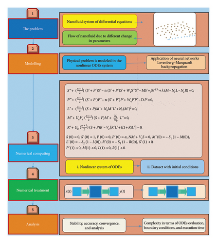
The governing terms of the nanofluid parameters, formulated through the SPLMR model, are presented in equation (1). To illustrate the variations in nanofluid characteristics, a graphical representation of the SPLMR model is provided in Figure 1, highlighting the structure of the proposed computational scheme. The main objective of this study is to obtain the solution of the system defined in equation (1) by integrating an intelligent computing framework based on ANNs. The state variables, system parameters, and their detailed descriptions are summarized in Tables 1 and 2.
| Variables | Description |
|---|---|
| S | Velocity profile |
| P | Velocity of field |
| M | Temperature |
| L | Concentration |
| R | Microorganisms |
| Factors | Description | Baseline values |
|---|---|---|
| D | Magnetic value | 0.1 |
| β | Modified Hartmann number | 0.1 |
| λ | Parameter of mixed convection | 0.1 |
| N1 = Nr | Ratio of buoyancy | 0.2 |
| N2 = Nc | Bioconvection Rayleigh value | 0.1 |
| N3 = Nt | Thermophoresis value | 0.1 |
| P1 = Pe | Peclet number | 0.1 |
| P2 = Pr | Prandtl number | 0.1 |
| N4 = Nb | The Brownian motion | 0.1 |
| L1 = Lb | Bioconvection Lewis’s value | 0.1 |
| L2 = Le | The impact of Lewis’s value | 1.4 |
| S1 | Thermal stratification Biot value | 0.1 |
| S2 | Solute stratification Biot number | 0.1 |
| S3 | Microorganisms’ stratification Biot number | 0.1 |
| Ω | Microorganisms difference | 0.01 |
| w | Cell swimming speed | 0.002 |
3.1. The Geographies of the Suggested Solver
- •
The solution of the mathematical model describing nanofluid flow in diverse environments is effectively presented through a novel application of an integrated intelligent computing approach based on ANNs.
- •
The accuracy and validity of the proposed ANN solver are demonstrated by comparing its results with the reference solutions obtained through the Runge–Kutta (RK) numerical method.
- •
The reliability of the model’s performance is further validated through statistical analyses, including the root mean square error (RMSE) and mean absolute deviation (MAD), across multiple applications of the ANN framework.
- •
The remainder of this paper is organized as follows: the proposed stochastic solver framework based on ANN is detailed in Section 3; the performance measures are discussed in Section 4; comprehensive results are presented in Section 5; and conclusions are summarized in Section 6.
3.2. Developed Technique
- •
Step 1: The formulation of a fitness function according to the error evaluation, carried out by building suitable ANN models.
- •
Step 2: The optimization of the fitness function to solve the mathematical model governed by equation (1).
4. Methodology and Performance Metrics
-
Phase 1: Evaluation of the nanofluid model through parameters like the input reference dataset for the feedforward neural network (FFNN).
-
Phase 2: Creation of the neural network backpropagation (NN-B) layer and training of the physics-informed machine learning (PML) models.
-
Phase 3: The solver proposed uses NN-BPML to solve the model.
The organization of the predictive scheme and accuracy with respect to the other equations resides in set equation (3). The dataset associated with the FFNN is here generated by the RK scheme as summarized in equation (6) and is then utilized for application in the SPLMR method. In this work, we construct the FFNN dataset using the “ND Solve” routine, with the RK algorithm applied to all SPLMR cases. To calculate all SPLMR cases, the structural layer of the FFNN is designed with a log-sigmoid activation function and includes 10 neurons in the hidden layers. A graphical representation of the FFNN model is provided in Figure 2. The FFNN is trained using backpropagation with the Levenberg–Marquardt method (LMM), based on the error function associated with the FFNN merit function. The MSE is used as a metric for performance, and the objective optimization function is defined through the LMM for each case.

Here, , Sl, and denote the approximate solution, reference solution, and mean solution for the ith input, respectively, while k represents the input grids. Additionally, R2, AE, and MSE are the essential parameters used for the complete proposed modeling.
The reference dataset for the SPLMR nanofluid model is developed over a period of 100 days, with a class interval of 1 day. The dataset was generated using Mathematica software to provide numerical results based on the ERK method for various scenarios of the SPLMR nanofluid model. The dataset contains compartmental values of S, P, L, M, and R into inputs. The data division for training, validation, and testing is set at 70%, 15%, and 15%, respectively.
5. Results
The comprehensive discussions of the attained outcomes to solve the nanofluid flow model equation (1) are shown in this section. The relative study with the RK outcomes explains the accuracy of the project method. Additionally, statistical outcomes are checked for the precision and accuracy of the project method.
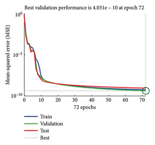
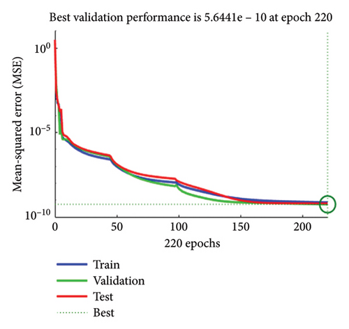
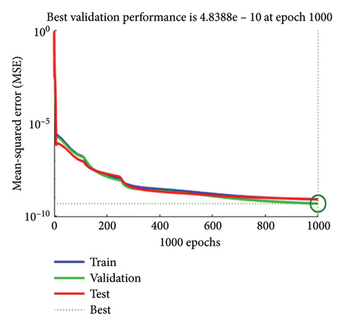
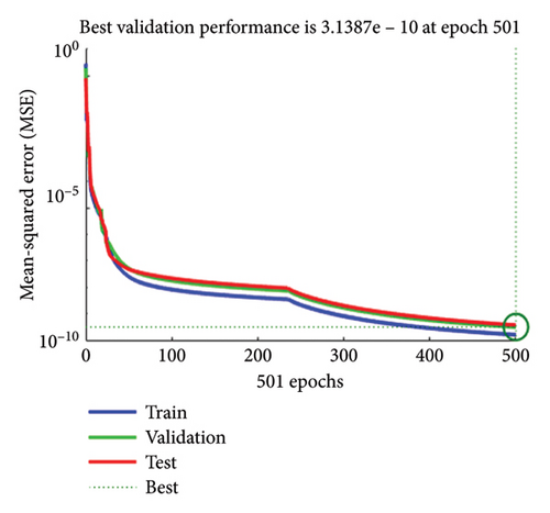
For each case of the SPLMR model for nanofluid, the results obtained through the proposed scheme are summarized in Tables 3, 4, 5, 6. The graphical representation of the performance analysis for all values of “⅄” is illustrated in Figures 3(a), 3(b), 3(c), 3(d). It is observed that in cases (1–4) of the SPLMR model, excellent performance is achieved across all cases, with the minimum MSE observed for Case 4 (best validation performance [BVP] = 3.138E − 10 at epoch 501). The smaller MSE values indicate the high accuracy and superior performance of the method. Specific MSE values for testing, validation, and training in all cases are provided in Table 7.
| Sr.# | Time | S | P | M | L | R |
|---|---|---|---|---|---|---|
| 1 | 0 | 8.36E − 06 | 5.38E − 07 | 1.05E − 05 | 8.63E − 06 | 3.43E − 05 |
| 2 | 10 | 6.02E − 06 | 2.73E − 07 | 2.44E − 06 | 1.17E − 05 | 3.79E − 05 |
| 3 | 20 | 1.90E − 05 | 4.57E − 08 | 9.05E − 06 | 1.59E − 05 | 1.73E − 05 |
| 4 | 30 | 1.43E − 05 | 9.11E − 08 | 5.38E − 06 | 1.28E − 05 | 7.52E − 06 |
| 5 | 48 | 1.79E − 05 | 1.66E − 07 | 8.65E − 06 | 1.32E − 05 | 5.43E − 06 |
| Sr.# | Time | S | P | M | L | R |
|---|---|---|---|---|---|---|
| 1 | 0 | 3.74E − 03 | −3.73E − 05 | 2.59E − 01 | 3.80E − 01 | 2.12E − 01 |
| 2 | 10 | 1.09E − 01 | 1.49E − 05 | 1.89E − 01 | 3.16E − 01 | 1.36E − 01 |
| 3 | 20 | 2.89E − 01 | −1.51E − 06 | 1.28E − 01 | 2.44E − 01 | 7.27E − 02 |
| 4 | 30 | 4.76E − 01 | −1.20E − 06 | 7.62E − 02 | 1.62E − 01 | 3.01E − 02 |
| 5 | 48 | 6.66E − 01 | −2.18E − 06 | −5.06E − 05 | 3.95E − 06 | −3.85E − 05 |
| Sr.# | Time | S | P | M | L | R |
|---|---|---|---|---|---|---|
| 1 | 0 | 1.13E − 02 | 2.17E − 07 | 1.85E − 01 | 4.51E − 01 | 1.52E − 01 |
| 2 | 10 | 3.00E − 01 | 1.55E − 07 | 1.14E − 01 | 3.88E − 01 | 7.37E − 02 |
| 3 | 20 | 7.50E − 01 | 1.43E − 07 | 6.48E − 02 | 3.03E − 01 | 2.27E − 02 |
| 4 | 30 | 1.21E + 00 | 1.54E − 07 | 3.36E − 02 | 2.02E − 01 | 4.08E − 03 |
| 5 | 48 | 1.71E + 00 | −9.29E − 07 | 2.62E − 06 | −6.62E − 05 | −2.67E − 05 |
| Sr.# | Time | S | P | M | L | R |
|---|---|---|---|---|---|---|
| 1 | 0 | 2.14E − 02 | 5.74E − 05 | 1.28E − 01 | 5.02E − 01 | 1.19E − 01 |
| 2 | 10 | 5.75E − 01 | 2.75E − 05 | 6.06E − 02 | 4.36E − 01 | 4.22E − 02 |
| 3 | 20 | 1.38E + 00 | 1.42E − 05 | 2.66E − 02 | 3.36E − 01 | 6.73E − 03 |
| 4 | 30 | 2.17E + 00 | 4.55E − 05 | 1.10E − 02 | 2.20E − 01 | 1.13E − 04 |
| 5 | 48 | 3.06E + 00 | −5.97E − 05 | −4.32E − 05 | −2.03E − 06 | −4.45E − 06 |
| Case | ⅄ | Time | Training | Testing | Validation | Perf. | Grad | Mu | Epochs |
|---|---|---|---|---|---|---|---|---|---|
| 1 | 0.1 | 04 | 5.325E − 10 | 8.525E − 10 | 4.031E − 10 | 4.031E − 10 | 9.867E − 08 | 1.00E − 08 | 72 |
| 2 | 0.4 | 07 | 7.320E − 10 | 6.409E − 10 | 5.644E − 10 | 5.644E − 10 | 9.907E − 08 | 1.00E − 08 | 220 |
| 3 | 0.8 | 26 | 8.419E − 08 | 1.766E − 07 | 3.659E − 08 | 4.838E − 10 | 3.349E − 07 | 1.00E − 08 | 1000 |
| 4 | 1.2 | 13 | 1.601E − 10 | 3.703E − 10 | 3.139E − 10 | 3.138E − 10 | 9.51E − 08 | 1.00E − 08 | 501 |
The state transition dynamics and the outcomes of the LMANNs for the SPLMR model are graphically presented in Figures 4(a), 4(b), 4(c), 4(d). Furthermore, the convergence parameters for all cases—execution time, MSE, backpropagation steps, performance, and epochs—are listed in Table 7, where the execution time also reflects the computational complexity of the developed approach.

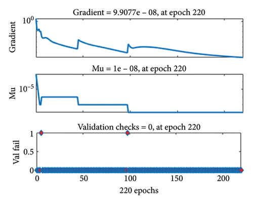
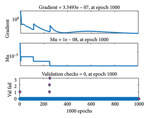
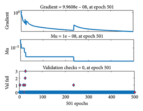
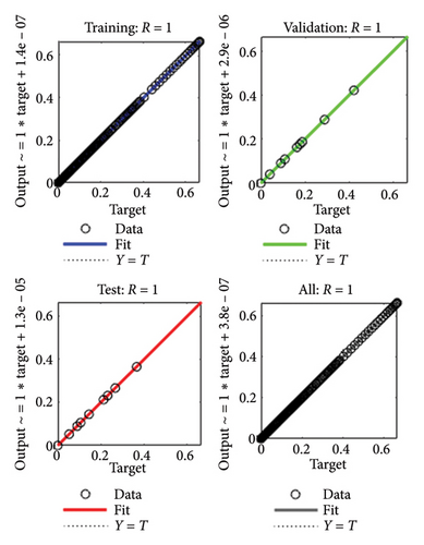
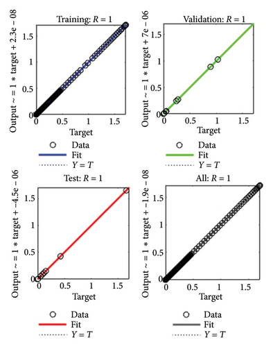
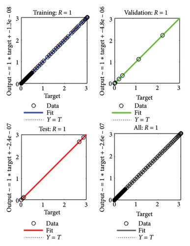
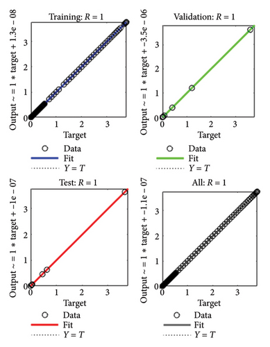
The gradient values and class size Mu for the different cases are approximately [9.867 × 10⁻⁸, 9.907 × 10⁻⁸, 3.349 × 10⁻⁷, and 9.51 × 10⁻⁸] and [10−8, 10−8, 10−8, and 10−8], respectively, as shown in Figures 4(a), 4(b), 4(c), 4(d). These small Mu values suggest strong convergence behavior. The comparison of regression plots for training, testing, and validation phases is shown in Figures 5(a), 5(b), 5(c), 5(d), where the regression value (R = 1) indicates an excellent correlation between the target and output values.
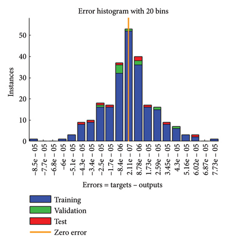
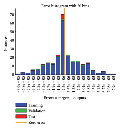
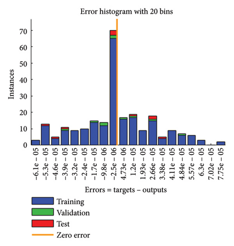
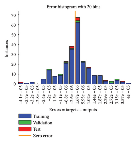
Error dynamics at each input point are further assessed using error histograms, graphically displayed in Figures 6(a), 6(b), 6(c), 6(d) for all cases of the SPLMR model. The errors around the zero-line bin 20 are taken as a reference, with corresponding values approximately [2.11 × 10⁻⁷, −2.5 × 10⁻⁶, −2.50 × 10⁻⁶, −2.6 × 10⁻⁶] for different cases.
The fitness plots comparing errors between target and output for testing, validation, and training are presented in Figures 7(a), 7(b), 7(c), 7(d) for all cases.
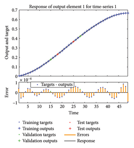
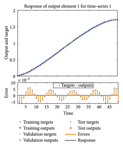
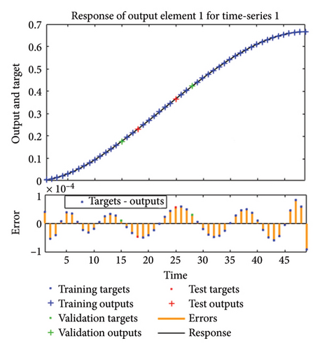
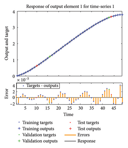
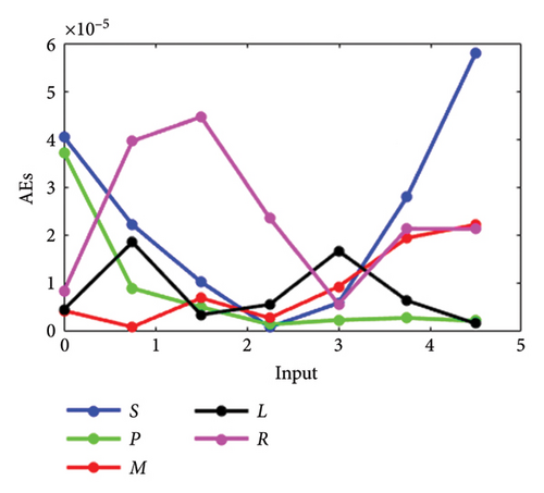
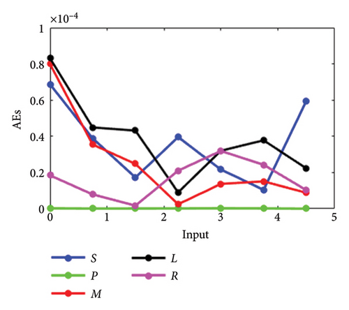
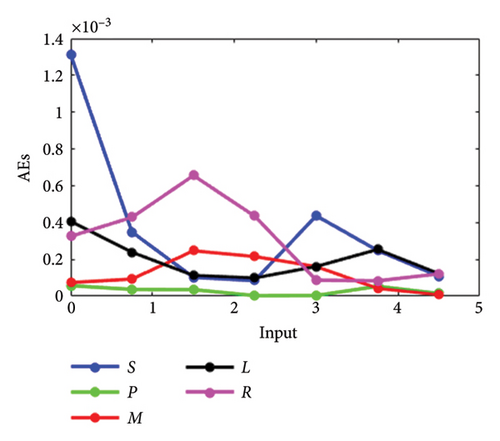
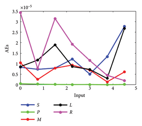
The results achieved via the LMANNs closely align with the reference ERK numerical solutions for each compartment of the SPLMR model. To assess precision, absolute errors are calculated and displayed in Figures 8(a), 8(b), 8(c), 8(d) and tabulated in Tables 3, 8, 9, 10.
| Sr.# | Time | S | P | M | L | R |
|---|---|---|---|---|---|---|
| 1 | 0 | 4.05E − 05 | 3.73E − 05 | 4.41E − 06 | 4.60E − 06 | 8.36E − 06 |
| 2 | 10 | 4.99E − 06 | 1.49E − 05 | 1.14E − 05 | 1.41E − 05 | 5.71E − 06 |
| 3 | 20 | 2.30E − 05 | 1.51E − 06 | 2.16E − 06 | 1.88E − 05 | 1.80E − 05 |
| 4 | 30 | 3.88E − 05 | 1.20E − 06 | 1.27E − 05 | 8.65E − 06 | 5.12E − 06 |
| 5 | 48 | 8.97E − 05 | 2.18E − 06 | 5.06E − 05 | 3.92E − 06 | 3.85E − 05 |
| Sr.# | Time | S | P | M | L | R |
|---|---|---|---|---|---|---|
| 1 | 0 | 6.87E − 05 | 2.17E − 07 | 7.98E − 05 | 8.30E − 05 | 1.84E − 05 |
| 2 | 10 | 4.60E − 05 | 1.55E − 07 | 1.68E − 05 | 1.93E − 05 | 5.81E − 07 |
| 3 | 20 | 3.38E − 05 | 1.43E − 07 | 1.34E − 05 | 3.17E − 05 | 9.03E − 06 |
| 4 | 30 | 1.39E − 05 | 1.54E − 07 | 2.06E − 05 | 3.48E − 05 | 2.28E − 05 |
| 5 | 48 | 5.34E − 05 | 9.29E − 07 | 2.62E − 06 | 6.62E − 05 | 2.67E − 05 |
| Sr.# | Time | S | P | M | L | R |
|---|---|---|---|---|---|---|
| 1 | 0 | 1.31E − 03 | 5.74E − 05 | 7.40E − 05 | 4.06E − 04 | 3.25E − 04 |
| 2 | 10 | 3.72E − 04 | 2.75E − 05 | 1.49E − 04 | 1.03E − 04 | 2.77E − 04 |
| 3 | 20 | 1.56E − 04 | 1.42E − 05 | 1.92E − 04 | 1.50E − 04 | 3.19E − 04 |
| 4 | 30 | 4.16E − 05 | 4.55E − 05 | 3.74E − 05 | 9.92E − 06 | 2.56E − 04 |
| 5 | 48 | 4.88E − 04 | 5.97E − 05 | 4.32E − 05 | 2.03E − 06 | 4.45E − 06 |
Finally, the accuracy analysis is based on statistical indicators including Min, Med, and SIR values for the SPLMR model, with detailed results presented in Tables 3, 8, 9, 10 for all cases.
5.1. Numerical Simulation With Interpretations
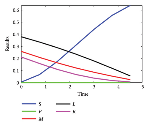
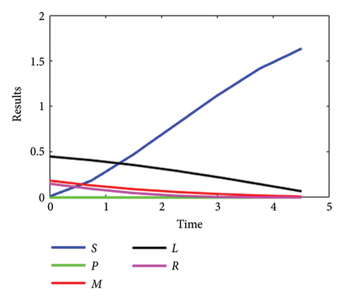
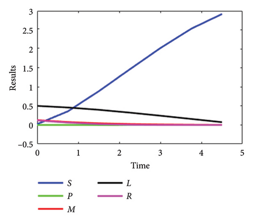
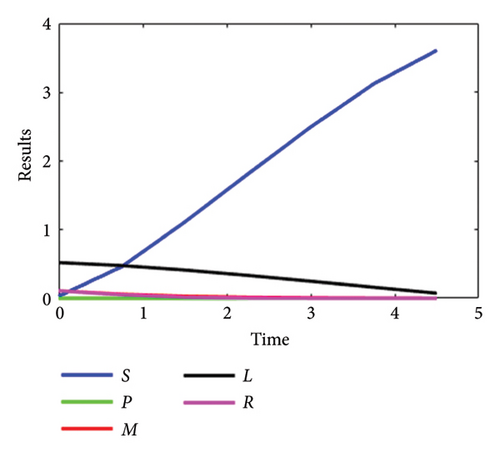
The detailed description of system (1-2) for the SPLMR model of nanofluid flow, using the developed LMANNs technique, is presented here. Various parametric quantities of the nanofluid model are analyzed through the proposed LMANNs framework, with comparative evaluations against reference numerical values for the SPLMR nanofluid model. Graphical results are provided to illustrate the comparative performance across all cases. For the variables S, P, L, M, and R, the numerical and graphical outcomes obtained via LMANNs are discussed to describe the flow behavior for different values of “⅄.” The corresponding numerical results are displayed in Figures 9(a), 9(b), 9(c), 9(d) and presented in Tables 4, 5, 6, 11 for all cases.
| Sr.# | Time | S | P | M | L | R |
|---|---|---|---|---|---|---|
| 1 | 0 | 2.95E − 02 | −5.38E − 07 | 1.09E − 01 | 5.19E − 01 | 1.08E − 01 |
| 2 | 10 | 7.23E − 01 | 2.73E − 07 | 4.43E − 02 | 4.49E − 01 | 3.28E − 02 |
| 3 | 20 | 1.71E + 00 | −4.57E − 08 | 1.66E − 02 | 3.43E − 01 | 3.52E − 03 |
| 4 | 30 | 2.68E + 00 | 9.11E − 08 | 6.09E − 03 | 2.22E − 01 | 1.04E − 04 |
| 5 | 48 | 3.79E + 00 | −1.66E − 07 | 8.65E − 06 | −1.32E − 05 | 5.42E − 06 |
5.2. Discussion
The physical characteristics of parameters such as λ, Lb, Nr, Pe, N, S2, Nc, S3, D, Pr, S1, Nb, Nt, β, and Le are graphically inspected for their effects on the velocity profiles (S, P), temperature distribution (M), concentration field (L), and microorganism concentration (R). Figures 3(a), 3(b), 3(c), 3(d) analyze the performance of the mixed convection parameter for different values of λ at n = 1, highlighting the influence of the magnetic parameter D on the velocity field S for n = 1. It is observed that increasing the magnetic parameter D results in a decrease in the velocity distribution S. The magnetic parameter D consistently reduces the velocity profile S due to the generation of a Lorentz force, which acts to resist the fluid motion.
The drag force impedes the flux, leading to a decrease in velocity as the magnetic field strength increases. Based on this, we hypothesize that the velocity of pseudoplastic nanofluid can be regulated by adjusting the magnetic field strength, denoted by D. To explore this, we compare the velocity distribution S of the fluid on a 3-D Riga plate with the modified Hartmann number β to investigate the induction effect. It is generally observed that a larger value of β results in a decrease in the velocity distribution S.
Figures 3(a), 3(b), 3(c), 3(d) illustrate the impact of the melting parameter N on S. As the magnitude of N increases, the velocity distribution SSS broadens for different values of the parameter λ. Furthermore, the influence of the concentration of nanoparticles Nc on S is considered, showing how variations in nanoparticle concentration influence the velocity distribution in the flow.
It is observed that the velocity distribution with respect to S for n = 1 increases with the enhanced value of Nc. The magnetic parameter D for n = 1 is noted to influence the performance with respect to P. Specifically, the behavior of the extended magnetic parameter D reduces the velocity field P. On the other hand, increasing the value of N leads to an increase in the velocity profile P, while the variation of λ also impacts the velocity distribution P. It is known that increasing λ improves the velocity field P compared to the 3-D Riga plate for n = 1 with variable sheet thickness.
To investigate the behavior of S1 on the rate of heat transfer, the parameter M for n = 1 can be represented. It is generally observed that increasing the value of the Biot number leads to an increase in the temperature distribution M. Furthermore, when evaluating the behavior of the energy field with respect to N for n = 1, it can be observed that a higher value of N increases the recorded temperature M.
The effects of the Brownian motion parameter Nb on the concentration of nanoparticles for n = 1 were examined. It is revealed that increasing the Brownian motion parameter Nb decreases the concentration curve L of nanoparticles. Regarding the behavior of Nt on the mass concentration of species L, an increasing trend in the concentration of nanoparticles L is observed. This occurs because, during thermophoresis, nanoparticles travel from the hot side to the cold side, so when λ increases, the concentration of nanoparticles L rises as well.
The hot matter moves away from the surface of the Riga due to the intensified mass field. The effect of the Lewis number (Le) on the mass transfer rate field (L) is observed. As the Lewis number (Le) increases, the concentration field (L) decreases, and this effect is influenced by the melting parameter (N), which modifies the concentration of species (L). It is found that for larger variations of the melting parameter (N), the concentration of L increases.
In addition, the concentration of L has been said to considerably increase the Biot numbers (S2 and S3), and the concentration of active microorganisms (R) decreases with increases in the Peclet number (Pe). The bioconvection Lewis number (Lb) defines this interaction since it changes with the microorganism concentration (R), and bioconvection Lewis number (Lb) declines with the increase in microorganism field (R). Bioconvection microorganism Biot number (S3) is given with respect to the concentration of microorganisms (R). Concentration of microorganisms is increased with the increase of bioconvection microorganism Biot number (S3). The local momentum coefficients, on the other hand, show increasing variations for larger values of D, Nr, and Nc, while, for increasing deviations of β, they tend to decrease.
6. Conclusions
ANN-based intelligent computing techniques are evolving to solve the proposed models for nanofluid flow in different environments. This is made possible because of approximation power enhanced by the global search efficiency of ANN with rapid improvement. The performance of the nanofluid flow dynamics in such an environment is thoroughly evaluated with the proposed numerical method based on ANN with hidden layer structure. The stochastic ANN solver has been validated by comparing its results with those of the RK numerical method, so proving it fit for nanofluid flow problems in varying environments.
Statistical analysis of the ANN performance is conducted using measures of central tendency. In the future, the proposed ANN-based algorithm holds promise as a powerful numerical solver for solving both stiff and nonstiff nonlinear systems, with potential applications in fields such as electric circuit theory, astrophysics, atomic physics, fluid dynamics, nanotechnology, plasma physics, and bioinformatics.
Conflicts of Interest
The authors declare no conflicts of interest.
Funding
The authors express their gratitude to Princess Nourah Bint Abdulrahman University Researchers Supporting Project number (PNURSP2025R913), Princess Nourah Bint Abdulrahman University, Riyadh, Saudi Arabia. Also, this work was supported by the Deanship of Scientific Research, Vice Presidency for Graduate Studies and Scientific Research, King Faisal University, Saudi Arabia [KFU251774].
Acknowledgments
The authors express their gratitude to Princess Nourah bint Abdulrahman University Researchers Supporting Project number (PNURSP2025R913), Princess Nourah bint Abdulrahman University, Riyadh, Saudi Arabia. Also, this work was supported by the Deanship of Scientific Research, Vice Presidency for Graduate Studies and Scientific Research, King Faisal University, Saudi Arabia [KFU251774].
Open Research
Data Availability Statement
The data supporting the findings of this study are available from the corresponding author upon reasonable request.


