AI-Powered Precision in Diagnosing Tomato Leaf Diseases
Abstract
Correct detection of plant diseases is critical for enhancing crop yield and quality. Conventional methods, such as visual inspection and microscopic analysis, are typically labor-intensive, subjective, and vulnerable to human error, making them infeasible for extensive monitoring. In this study, we propose a novel technique to detect tomato leaf diseases effectively and efficiently through a pipeline of four stages. First, image enhancement techniques deal with problems of illumination and noise to recover the visual details as clearly and accurately as possible. Subsequently, regions of interest (ROIs), containing possible symptoms of a disease, are accurately captured. The ROIs are then fed into K-means clustering, which can separate the leaf sections based on health and disease, allowing the diagnosis of multiple diseases. After that, a hybrid feature extraction approach taking advantage of three methods is proposed. A discrete wavelet transform (DWT) extracts hidden and abstract textures in the diseased zones by breaking down the pixel values of the images to various frequency ranges. Through spatial relation analysis of pixels, the gray level co-occurrence matrix (GLCM) is extremely valuable in delivering texture patterns in correlation with specific ailments. Principal component analysis (PCA) is a technique for dimensionality reduction, feature selection, and redundancy elimination. We collected 9014 samples from publicly available repositories; this dataset allows us to have a diverse and representative collection of tomato leaf images. The study addresses four main diseases: curl virus, bacterial spot, late blight, and Septoria spot. To rigorously evaluate the model, the dataset is split into 70%, 10%, and 20% as training, validation, and testing subsets, respectively. The proposed technique was able to achieve a fantastic accuracy of 99.97%, higher than current approaches. The high precision achieved emphasizes the promising implications of incorporating DWT, PCA, GLCM, and ANN techniques in an automated system for plant diseases, offering a powerful solution for farmers in managing crop health efficiently.
1. Introduction
Tomato is an important agricultural product, accounting for 15% of global vegetable consumption, with an average annual per capita consumption of 20 kg [1]. Fresh tomatoes are one of the most commercially important crops, with world production exceeding 170 million tons per year [2]. But there are major challenges in growing tomatoes, especially the risk of several leaf diseases. These consist of bacterial spot, early blight, late blight, Septoria leaf spot, yellow leaf curl virus, leaf mold, spider mites, mosaic virus, and target spot, which jeopardizes the world tomato industry [3]. Most economies in the world lost a lot of tomato due to diseases with an annual average reduction of 10% according to the Food and Agriculture Organization of the United Nations [4].
Tomato crops face enormous threats from diseases including bacterial spot, Septoria leaf spot, late blight, and yellow leaf curl virus in areas like Bangladesh. These diseases are particularly serious as they start in the leaves and quickly affect the whole plant [5, 6]. Charged with the same symptoms, they are often misdiagnosed due to this very reason [7]. As a result of these objectives, it is necessary to create an efficient and effective mechanism for the timely and accurate recognition and classification of tomato leaf diseases in order to maintain agricultural productivity.
Routine diagnostic practices, including visual inspection and laboratory-based microscopic examination, are labor-intensive, subjective, qualitative, and susceptible to human errors and therefore not ideal for monitoring large samples of animals [8]. A manual inspection relies heavily on human skills to diagnose diseases on tomato leaves, yet these techniques are labor-intensive, variable, and are not always reliable when differentiating close disease look-alikes. These methods are challenging to implement on a large scale due to an increase in the cost of expertise hire throughout [9, 10]. The microscopic laboratory investigations with molecular and immunological techniques demand high-end experimental facilities, thus presenting a considerable effort toward the practical use of these resources for the agricultural sector [11]. Such limitations leave a gaping need for rapid and accurate disease identification and classification systems. Therefore, it is indispensable to establish those kinds of systems for the sustainability and efficiency of tomato cultivation, especially in Bangladesh, where the bacterial diseases of tomato leaves are a key concern [12].
With the recent developments in artificial intelligence (AI) and digital image processing (DIP), these emerging technologies have great potential for the automated identification and classification of plant diseases [13]. As such analyses can be arduous and challenging when performed using traditional techniques, deep learning (DL), a branch of AI, has become an important tool for these tasks and can offer remarkable benefits. DL methods, especially convolutional neural networks (CNNs), are efficient in extracting necessary features from images and do not require any manual feature engineering [14]. Several studies have shown that CNNs can autonomously extract spatial and textural features of the disease directly from the leaf images, and classification accuracy outperformed traditional machine learning techniques [15, 16]. Nevertheless, despite the success, traditional DL methods have limitations, which need to be addressed for further improvement. A particularly important challenge is their black-box nature [17, 18], which prevents transparency and does not allow understanding the disease patterns and complicates the prediction of novel or atypical cases. In addition, DL models generally tend to need a considerable amount of training data to effectively learn relevant features, and to obtain a well-balanced corpus of labeled data in diverse habitats is expensive and can take long time, especially for specialized applications such as tomato leaf disease detection. Such a lack of data increases the risk of overfitting [19]. Additionally, the deployment of DL models in resource-constrained settings necessitates significant computational requirements, hardware, and expertise. Moreover, these models tend to be sensitive to any fluctuation in the input data, such as lighting conditions, camera perspectives, and image distortion, which negatively influence the classification accuracy and decrease the model robustness in real-world applications [20, 21].
In this work, to overcome these limitations, we propose our solution, a two-phased approach separating feature extraction from classification, utilizing classical image processing techniques together with a tight neural network model for classification. Discrete wavelet transform (DWT) and gray level co-occurrence matrix (GLCM) are used for feature extraction, and principal component analysis (PCA) is used for dimensionality reduction. DWT was selected to extract both spatial and frequency-domain features, which is useful to identify texture differences between a healthy and diseased leaf [22]. According to textural property extraction using features, GLCM demonstrates the spatial relationship between pixels which aids in differentiating disease patterns [23]. This enables PCA to compress the feature space to only those features that are meaningful for task, thereby reducing complexity [24]. For the classification phase, artificial neural networks (ANNs) were chosen because they can provide generalization and are easy to use for multiclass classification problems [25]. We then perform classification and classification analysis using an ANN. ANN can create nonlinear mappings between extracted features and disease classes, making it a strong candidate for classification. ANNs have higher expressiveness than traditional classifiers [26] (e.g., support vector machines (SVMs) and random forests (RFs)), allowing to fit complex data, which makes them well-suited for the problem of multidisease detection [27].
- 1.
Uncovering hidden disease indicators via multilevel image preprocessing.
- 2.
Intentional K-means to segment the affected area.
- 3.
Exposing the disease signatures through mixed feature extraction (DWT and GLCM) and dimensionality reduction (PCA) methods.
- 4.
Chi-square and Fisher’s score for key feature identification.
- 5.
Optimized ANN for the classification of diverse diseases.
- 6.
Evaluating the proposed approach against the existing integrated feature extraction techniques and high-end ML and DL approaches.
The rest of the article is organized as follows. In Section 2, we review recent literature on the detection and classification of plant diseases. Section 3 describes the materials and methods followed during the study (experimental design and data acquisition). Section 4 discusses the results with analytical representation. Section 5 presents the results and compares them with existing state-of-the-art techniques. Lastly, Section 6 reviews the basic findings and contributions to the field, before concluding the study.
2. Literature Review
In precision agriculture, automated diagnosis of plant disease is an important research field. The objective is to create accurate ways to detect and classify diseases that exist in plants which could assist farmers dealing with their crops and increasing yield [28]. Over the years, plant disease detection has undergone a journey that has made a further leap from traditional machine learning approaches to DL and hybrid solutions.
Some studies have addressed plant disease diagnosis using classical ML algorithms, most often applying a mixture of extraction and classification methods. Algorithms commonly used include SVMs, RFs, and decision trees (DTs). A computationally efficient and accurate framework to reduce feature extraction techniques (color histograms, Hu moments, Haralick features, and local binary patterns) was created by Basavaiah and Arlene Anthony [29]. RF and DT were the employed classifiers reaching 94% accuracy with the former and 90% with the latter on the proposed framework. Gadekallu et al. [30] introduced a hybrid methodology employing PCA-based whale optimization algorithm to identify and categorize tomato leaf diseases, achieving significant enhancements in accuracy. Mathew et al. [31] used texture features obtained by GLCM and SVM classification with an accuracy of 95.99%. But this would be difficult given the texture complexity between and within diseases. Similarly, in [32], a hybrid of DWT and color histograms was established and then RF was applied for classification that reached an accuracy of 98.63%. While this approach efficiently encapsulates both frequency and color information, it might struggle because of the large dimensionality of the feature space.
Unlike traditional machine learning approaches, DL techniques have capability to automatically learn features from raw data, particularly excelling in image-based plant disease diagnosis through CNN [33]. Balaji et al. [34] introduced a genetic algorithm–based customized CNN that achieved commendable accuracy, exceeding 95% in classifying leaf diseases. Roy et al. [35] developed a novel PCA DeepNet framework, combining classical machine learning models with a customized deep neural network (DNN). This framework achieved a classification accuracy of 99.60%, an average precision of 98.55%, and an impressive intersection over union (IOU) score of 0.95 in detection. Similarly, Ullah et al. [36] proposed the DeepPlantNet framework, which efficiently detected and classified plant diseases with an accuracy of 97.89%. Altaluk et al. [37] presented a hybrid approach integrating CNN, a convolutional block attention module (CBAM), and SVM, yielding an accuracy of 97.2%. Guerrero-Ibaez and Reyes-Muoz [38] combined CNN with generative adversarial networks (GANs), achieving an accuracy of 99.64% for leaf disease classification.
Multimodel transfer learning has been extensively researched to reduce the need for exhaustive labeled data and computational resources, yet transfer learning models are not always capable of achieving the level of specificity in features necessary to answer domain-specific questions. Paymode et al. [39] proposed a VGG16-based CNN model as a detection tool for plant diseases with 95.71% accuracy, though Ansari in [40] developed a deep CNN-based dilated ResNet-18 model for the same problem and yielded 99.1% accuracy. Al-Gaashani et al. [41] designed a hybrid model using MobileNetV2 and NASNetMobile integrated with kernel PCA to achieve 97% accuracy. Rajamohanan and Latha [42] developed a novel transfer learning model using computer vision (YOLOv5), with an accuracy of 93%. Using transfer learning approach, Uhasree and Pradeepini [43] developed a model to predict diseases in tomato leaf based on InceptionV3 architecture and obtained an accuracy of 98%. Debnath et al. employed a transfer learning approach using the EfficientNetV2B2 model, achieving a notable average weighted validation accuracy of 99.22% [44]. However, even achieving high accuracy during testing, these models may overlook those particular features providing distinctiveness to different plant diseases as they were usually pretrained on massive generic datasets such as ImageNet where millions of images have thousands of classes. These datasets are not plant-specific but provide a diverse set of objects, animals, and scenes. Hence, the attributes learned by the model support the identification of nonplant diseases.
Recent works have proposed hybrid methods that combine classical visual descriptors with DL to enhance the accuracy while maintaining lower computational costs. Kanabur et al. [45] utilized DWT and GLCM feature extraction combined with CNN for classification and achieved 99.09% accuracy while minimizing the computational requirements of a pure DL model. Kaur et al. [46] proposed a Hybrid-DSCNN model for segmenting infected regions in tomato leaves that achieved an accuracy of 98.24%. Although these hybrid models provide advancements with respect to accuracy, they tend to demand substantial computational capacity. Yag and Altan [47] showed the potential of integrating DWT with CNN, resulting in 99.56% accuracy; however, they noted the high computation costs during processing and training of the complex models.
This review shows the different approaches to automatic plant disease detection and the pros and cons. Through the synergy of multifeature extraction technology and optimized neural network integration, our work contributes new methods of high accuracy and practicality in the field.
3. Materials and Methods
3.1. The Proposed Leaf Disease Detection and Classification System
This work presents a new tomato leaf disease diagnosis approach through hybridized advanced feature extraction and an optimized ANN. It deals with four important tomato foliar diseases: Septoria leaf spot, late blight, yellow leaf curl virus, and bacterial spot. The high-level flow of the proposed system and its hierarchical transformation from raw image data to disease classification is shown in Figure 1.
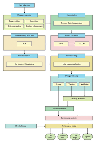
In this study, we used a dataset based on PlantVillage.com, displaying different types of diseases on tomato leaves. A number of preprocessing techniques were applied to improve the quality of the inferences from images. Image scaling was applied first to make sure all of the samples were the same dimension. The next conversion was color conversion, which was used to convert the original RGB images to grayscale, such that texture details of the images were emphasized while at the same time the effect of the color components of the images was reduced. The Otsu binarization effect captured above was applied to automatically select the threshold that separates the leaf features in the image from the background noise. The preprocessed images were used as a base to extract specific features, beginning with K-means clustering dividing the images and revealing diseased regions for in-depth observation. We use a hybrid feature extraction approach that entails decomposing images onto frequency bands to grasp coarse, medium, and fine textures, GLCM to compute spatial interrelationships and capture disease-specific patterns, and PCA to retain the most important features while discarding redundant ones. Together, these methods generated 13 statistical features for each image. Feature relevance was assessed using chi-square and Fisher scores, indicating that, among all, the IDM feature had the lowest classification relevance. Therefore, the study was designed to be robust and efficient: hence the focus was on the 12 most contributing features. Then, an enhanced ANN classifier is employed to differentiate between four diseases according to such features. Thus, the tomato leaf disease preprocessing, image processing, feature extraction, and automatic classification, all consisting of a classification workflow, showed a better approach for the automation of tomato disease diagnosis, which may improve the practice in horticulture and crop productivity.
3.2. Tomato Leaf Diseases
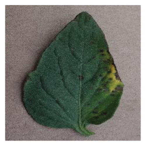
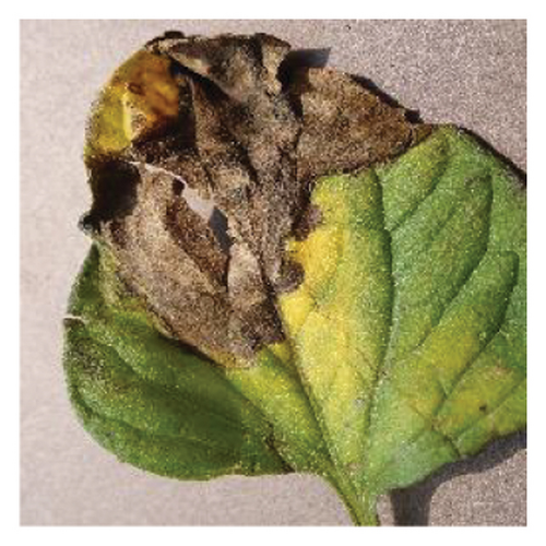
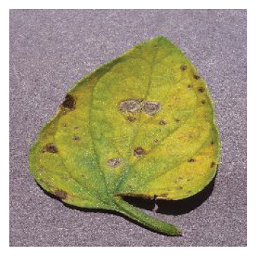
From little viruses like the DNA-driven yellow leaf curl virus, spread by devious whiteflies, to damaging bacteria like Campylobacter, which brings on the growth of dark scabs on damaged leaves, tomato plants face myriad foes. Fungi thrive in wet conditions, as evidenced by common plant diseases such as late blight, which shows up as smelly green-black spots on leaves, and Septoria leaf spot, which creates dark-edged circles on leaves. These fungal infections represent potential threats to agricultural productivity and economic stability, making them key challenges in crop management and plant pathology [48]. Figure 2 shows sample images of some infected tomato leaves.

3.3. Data Collection
In this work, we used the publicly accessible PlantVillage dataset, which is a salient dataset for plant disease research. It consists of 9014 images of tomato leaves in 256 × 256 pixel resolution. The images are divided into four disease class categories: bacterial spot, Septoria leaf spot, late blight, and curl virus. The distribution of images across these categories is shown in Table 1.
| # | Name of the class | Number of samples |
|---|---|---|
| 1 | Curl virus | 3208 |
| 2 | Bacterial spot | 2127 |
| 3 | Late blight | 1908 |
| 4 | Septoria leaf spot | 1771 |
| Total | 9014 | |
3.4. Image Preprocessing
Prior to the disease categorization, images of tomato leaves pass through a wide preprocessing phase before being used for analysis as represented in Figure 3. In this stage, various methods are used to improve the information of an image, decrease computational cost, and perform accurate identification of the disease. Table 2 shows the parameters utilized throughout the preprocessing and feature extraction stages, and this allows for this work to be reproducible.

| Stage | Method/technique | Parameters |
|---|---|---|
| Preprocessing | Image scaling | Dimensions: 200 × 200 pixels |
| Gaussian smoothing | Kernel size: 5 × 5, standard deviation (σ): 1.0 | |
| Otsu binarization | Thresholding method | |
| Contrast enhancement | Histogram equalization | |
| Feature extraction | DWT | Wavelet: Haar, levels: 1 |
| GLCM | Distance: 1 pixel, directions: 0°, 45°, 90°, 135° | |
| PCA | Number of components: 12 | |
3.4.1. Image Resizing
Data and computing viability are key ingredients in our workflow. Image scaling is the first step, which shrinks each image to 200 × 200 pixels. We also resize our images, which is worthwhile, as we need the dimensions of the training and test images to match, so they have similar pixel values, so our classifier has a fair field.
3.4.2. Smoothing
Many leaf diseases exhibit subtle textural differences, which are often relied on for detection. To address these subtleties, a smoothing filter homogenizes the pixel intensity values throughout the image, permitting a coherent and noise-free representation. Gaussian smoothing (σ: 1.0; kernel size: 5 × 5): To reduce noise while maintaining edges, we applied Gaussian smoothing to each image. This approach reduces unwanted detail and emphasizes key patterns of disease, allowing for improved feature extraction.
3.4.3. Otsu Binarization
The probabilities of the number of pixels in each class at threshold t are represented by ωbg(t) and ωfg(t), and the variance of color values is denoted by σ2.
3.4.4. Contrast Enhancement
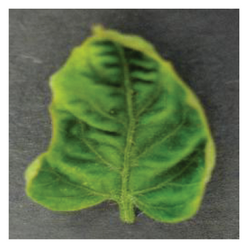
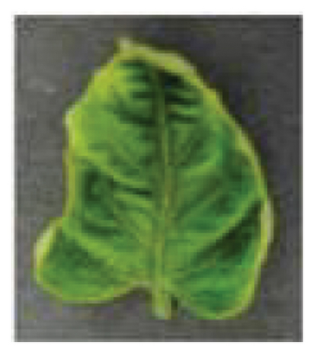
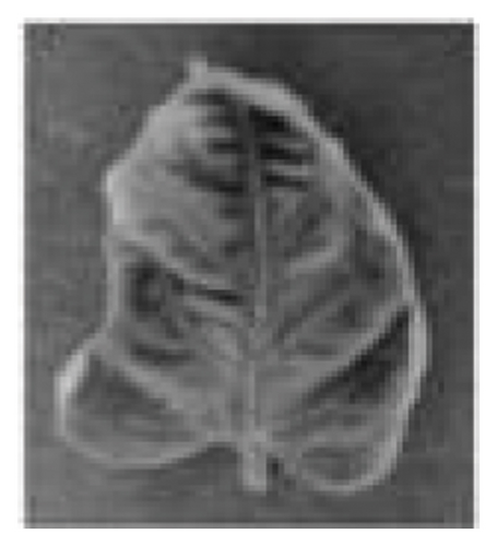
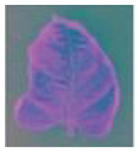
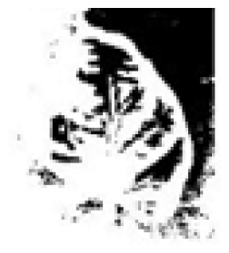
The histogram equalization contrast enhancement method accentuates the small intensity variations in preprocessed images to improve the clustering algorithm. This method increases the contrast range to enable the clustering algorithm to be able to detect and distinguish previously nonvisible patterns of disease, thus facilitating the identification of the data. It intensifies the awareness of the visual field, enabling the spotting of even the subtlest signs of disease. The preprocessing steps applied to a Septoria leaf spot–infected leaf are shown in Figure 4.
3.5. Segmentation
In equation (2), O = objective function, M = number of cases, N = number of clusters, Cj = centroid of clusters j, xi = case i, and is the distance function.
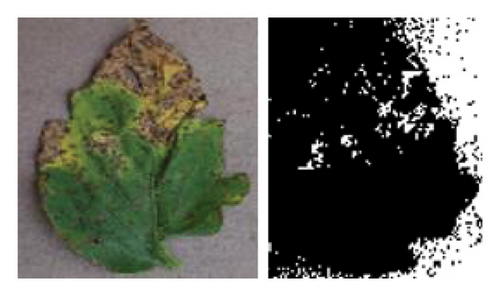
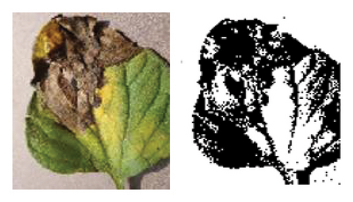
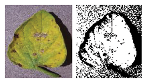
Figure 5 illustrates the K-means algorithm’s role in our workflow. It begins by importing and converting the image from RGB to Lab∗ color space. This transition separates brightness (“L∗”) from color information (“a∗” and “b∗”), enabling the algorithm to focus on color variations relevant to the condition. The K-means algorithm then groups pixels by moving them toward their nearest cluster centroids, which adjust to fit their new pixel groups. This iterative process continues until a stable configuration is reached, dividing the image into three distinct parts [51].

The respective index value associated with each pixel represents the observation returned by the clustering algorithm indicating predicted membership to one of the k (k = 3) clusters corresponding to the separate regions available in the image: healthy leaf tissue, disease area, and background. These segmented portions of the input image are utilized for feature extraction and disease detection to ensure accurate diagnosis. As shown in Figure 6, the K-means clustering algorithm is applied to leaf segmentation. The left image represents the original leaf, while the right image depicts the clustered leaf, demonstrating the algorithm’s effectiveness in feature extraction and classification. The right image showcases the segmented outcome, where various colors identify unique clusters identified through the algorithm.

3.6. Feature Extraction and Dimensionality Reduction
Accurate classification of disease requires the extraction of valuable information from the preprocessed images. Feature extraction was performed using both DWT and GLCM, while PCA was used for dimensionality reduction. In general, DWT decomposes images into frequency-oriented components and captures texture features that provide signs of disease, while GLCM analyzes spatial relationships between the presence of pixels within an image to distinguish patterns indicative of healthy and diseased tissue. PCA condenses these features into a smaller, more interpretable set. With this method, we obtain three distinct statistical features from every image.
3.6.1. DWT

The DWT decomposes the input image into distinct frequency components that can be represented by four sub-bands [32].
Low-low (LL) sub-band: It contains approximation coefficients, representing low frequency. Best version coarse representation retains the top properties.
High-low (HL) sub-band: This sub-band contains the horizontal detail coefficients that record the high-frequency coefficients in the row level (horizontal direction) and low frequency in the column level (vertical direction). This one does edge detection and more specifically vertical edges in the image.
Low-high (LH) sub-band: The LH sub-band represents the vertical details, taking the low-frequency components along the rows (horizontal direction) and high-frequency components along the columns (vertical direction). It detects the horizontal edges in the image.
High-high (HH) sub-band: This sub-band represents diagonal detail coefficients, which are the high-pass components of the image along both the rows and columns. This accentuates the diagonal edges and also the fine details in the image.
The LL sub-band holds a significant amount of the original image data, whereas the HL, LH, and HH sub-bands encode edge and the detail data, respectively. Multiple sub-bands are significant in successful feature extraction, contributing to multiresolution texture and structural data types.
3.6.2. GLCM
Texture offers valuable information regarding the presence of diseases in the images. To do this, we refer to the GLCM, that is, a matrix concerned with gray levels for pairs of neighboring pixels. GLCM diagnosis utilizes 8 × 8 matrix analysis to ascertain co-occurring patterns that expose textural features suggestive of disease. A leaf with a disease may reflect very different values for the bright and dark pixels, making it easy to detect lesions or other color changes. GLCM records these slight variations, revealing texture details that the human eye cannot perceive [45].
3.6.3. PCA
We also applied PCA after extracting a full set of features with DWT and GLCM to reduce the dimensions of the feature data. PCA changes the original feature space to a new space of orthogonal components, where each of those components is called a principal component, such that the principal components capture as much of the variance of the original space as possible. Through this process, redundant and less informative features are discarded, while the most essential features for classification are preserved. This, in turn, reduces the computational burden and the risk of overfitting, so the resulting model generalizes well to unseen data. Then it passes the resulting principal components to the classifier for training and evaluation [35].
3.6.4. Extracted Statistical Features
3.7. Feature Selection
Table 3 outlines the features alongside their chi-square and Fisher scores.
| SL. | Features | Chi-square score | Fisher score |
|---|---|---|---|
| 1 | Contrast | 1.25825 | 8.31054 |
| 2 | Correlation | 1.03814 | 7.92778 |
| 3 | Energy | 0.83647 | 7.58341 |
| 4 | Homogeneity | 0.80528 | 7.50413 |
| 5 | Entropy | 0.61273 | 7.41873 |
| 6 | Variance | 0.58243 | 7.09821 |
| 7 | Mean | 0.57732 | 6.75843 |
| 8 | Standard deviation | 0.54928 | 6.57814 |
| 9 | Skewness | 0.52554 | 6.48718 |
| 10 | Kurtosis | 0.51378 | 6.46023 |
| 11 | RMS | 0.48549 | 5.79274 |
| 12 | Smoothness | 0.43857 | 4.58271 |
| 13 | IDM | 0.00214 | 0.05214 |
- Note: The bold value indicates that GLCM-based IDM (Inverse Difference Moment) was discarded as it exhibited the weakest chi-square and Fisher scores, reflecting its limited utility for feature selection.
By reviewing feature importance scores, we determined that there were 12 traits that stood above the rest in significance. The selected features were, indeed, the most useful among the tomato leaves of the four diseases. An additional feature named IDM was also excluded due to low discriminative power and redundancy with other features. Among the individual features, IDM consistently ranked lower in importance than many other features and provided minimal unique information. Also, IDM highlights local homogeneity and was highly correlated with GLCM texture feature contrast and correlation. IDM would have added unnecessary complexity while not improving performance. We excluded IDM, resulting in a simplified feature set that helped to improve model accuracy (99.97%) and computational efficiency.
3.8. Feature Scaling
Here, xnormal represents the normalized feature value, x is the original feature value, xmin is the minimum value within the feature set, and xmax is the maximum value within the feature set.
3.9. Architecture of the Proposed AI Model
For the multiclass classification of leaf diseases, we use an ANN, due to its significant functionality for varying correlation of data in a complex manner. As shown in Figure 8, the suggested ANN architecture adopted a feed-forward topology in which information is passed through several layers, each important to the classification. The first layer is the input layer with 12 neurons, and each unique one represents a single relevant feature selected from the preprocessed images, allowing the ANN to analyze the most descriptive information in the image for diagnosis. Next to the input layer, a hidden layer with 15 neurons connects intermediary neurons that apply nonlinear transformations to the incoming data. This layer studies complex relationships and knows the health context in detail. The output layer has four neurons that classify a tomato leaf as having a disease. The specific neural structures are created to identify the unique signals for each disease that the ANN can interpret accurately for highly confident diagnostics. Such a targeted design can revolutionize farming and protect crops by providing accurate disease classification.
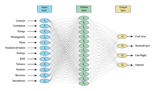
By effecting a careful procedure in establishing a comprehensive dataset that has been further segmented into specific training, validation, and testing subsets with which we trained our proposed ANN, we ensured that our ANN arrives at accurate resolutions. We utilized the Adam optimizer in the training phase to iteratively update the internal parameters of the network so that performance improved. Through this continuous training process, the ANN hones its skills, learning to recognize even the slightest signs of disease.
3.10. Validation Techniques
We implemented the following validation strategies to build a strong model that could generalize well on unseen data.
Holdout validation: The data were randomly split into three sets: 70% (6310) for training, 10% (902) for validation, and 20% (1802) for testing. The validation set was used to tune hyperparameters and as a way to observe generalization capabilities of the model, during training.
K-fold cross-validation: Besides holdout validation, we also used k-fold cross-validation with k = 5 to ensure that the model evaluation is comprehensive. We split the dataset into five equal portions and trained and validated the model five times. In every iteration, it treated a new fold as validation set and all other folds as training set. Using it helped to reduce variance and provided a better estimate of the performance of the model. An effective way to improve performance while preventing n-fold overfitting was to utilize holdout validation in conjunction with k-fold cross-validation.
3.11. Evaluation Metrics
In order to deeply evaluate the effectiveness of the suggested method, we make use of the multiclass confusion matrix, which offers a comprehensive perspective of model performance in multiclass classification. This N × N grid provides a rich landscape of the models performance, where it is accurate, where it is strong, and where it is weak. A confusion matrix provides a cross-tabulation of predictions versus actual disease diagnoses. True positive (TP) defines diseased leaf that is detected by a model as the diseased leaf and true negative (TN) describes healthy leaves that are correctly detected as healthy. However, there is a challenge in false positives (FPs), wherein healthy leaves are mistakenly identified as diseased, a scenario akin to friendly fire incidents, and false negatives (FNs), wherein diseased leaves are not identified, evading the model’s defense.
3.12. Experimental Settings
In this section, we detail the experimental settings used in our study to ensure transparency and reproducibility of our results.
3.12.1. ML and DL Model Configuration
In order to improve the classification stage even more, we tested extra classifiers besides the proposed ANN, including traditional methods based on machine learning as well as configurations based on DNNs. To guarantee a fair comparison, the classifiers were evaluated using the identical set of 12 selected features. The extended analysis was aimed at finding the best classification model for the task. Table 4 shows the parameters used in classification stage.
| Stage | Method/technique | Parameters |
|---|---|---|
| Classification | SVM | Kernel: RBF, C: 1.0, gamma: 0.1 |
| RF | Trees: 100, depth: 10 | |
| KNN | k: 5 | |
| ANN | Input layer: 12 neurons, hidden layers: 1-2, output layer: 4 neurons | |
| Activation functions: sigmoid (hidden layer), softmax (output layer) | ||
| Optimizers: SGD, Adam, RMSprop | ||
| Learning rate: 0.001 | ||
| Batch size: 64 | ||
| DNN | Hidden layers: 3-4, activation: ReLU, optimizer: Adam | |
| Hyperparameter optimization | Grid search for each classifier |
3.12.2. Computing Platform and Resources
The experiments were conducted on a computing platform equipped with the resources shown in Table 5.
| Criteria | Explanation |
|---|---|
| Processor | Intel Core i7-9700K CPU @ 3.60 GHz |
| RAM | 32 GB DDR4 |
| GPU | NVIDIA GeForce RTX 2080 with 8 GB GDDR6 |
| Operating system | Microsoft Windows 10 Home |
| Software framework | MATLAB R2020a for neural network training and evaluation |
4. Results and Analysis
4.1. Model Optimization
The first study had a database with 9014 samples, each being represented as a 12-dimensional vector of statistical properties. A randomized split of the existing dataset into training, validation, and testing subsets allowed a robust and unbiased evaluation of the approach. In particular, 70% of the samples (6310) were designated to the training set, where the model ingests the relationships among input attributes and class labels. The rest 30% was then divided into a validation set (10%, 902 samples) to tune hyperparameters and a testing set (20%, 1802 samples) used to evaluate the model’s performance when applied to new samples.
We applied a 5-fold cross-validation process to increase the robustness and reliability of our proposed model. Table 6 presents a summary of the results obtained using the 5-fold cross-validation. The performance measures are averaged across the 5-folds, with standard deviations informing the reader of the variance in the model’s performance.
| Fold | Accuracy (%) | Precision | Recall | F1 score | RMSE |
|---|---|---|---|---|---|
| 1 | 99.95 | 0.9995 | 0.9995 | 0.9995 | 0.00105 |
| 2 | 99.96 | 0.9996 | 0.9996 | 0.9996 | 0.00104 |
| 3 | 99.97 | 0.9997 | 0.9997 | 0.9997 | 0.00103 |
| 4 | 99.96 | 0.9996 | 0.9996 | 0.9997 | 0.00106 |
| 5 | 99.96 | 0.9996 | 0.9996 | 0.9996 | 0.00104 |
| Mean | 99.97 | 0.9997 | 0.9997 | 0.9997 | 0.00104 |
| Std. dev. | 0.011 | 0.00011 | 0.00011 | 0.00011 | 0.000013 |
The network that achieved the lowest RMSE value (0.00107 after 67 iterations) is the one that had 15 hidden neurons (see Table 7), suggesting that it was the optimal level of model complexity, generalizability, or bias/variance trade-off. This ideal architecture was determined based upon training the model with the scaled conjugate gradient backpropagation method, which helped provide greater specificity in differentiating between diseases.
| Number of hidden neurons | Iterations | RMSE |
|---|---|---|
| 10 | 48 | 0.00412 |
| 15 | 67 | 0.00107 |
| 20 | 31 | 0.00505 |
| 25 | 36 | 0.00397 |
| 100 | 51 | 0.00366 |
- Note: The bold value provides focus on achieving the optimal results, characterized by the lowest RMSE, by selecting the appropriate number of neurons and iterations.
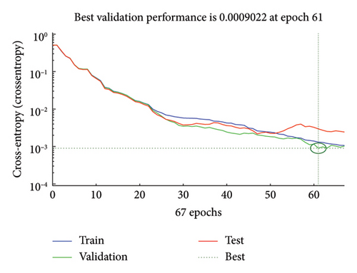
This high MSE shown in Figure 9 is expected as the network is initially “learning.” Eventually, this MSE shrinks a lot around epoch 61, when the error falls below 0.0009022. This reduction identifies that the model learns well over the data and generalizes it properly from the training data. Since the MSE after epoch 61 stabilizes, the model has most probably not overfitted and is giving the best performance. In fact, training beyond this point probably did not improve generalization and may have even resulted in overfitting, since continuing at this point would have continued to minimize training error at the cost of validation performance. These are all excellent signs of the architecture and training parameters chosen, validating that the model is not overfitting and that the parameters chosen are useful in pursuit of a model tailored toward practical deployment in real-world applications.
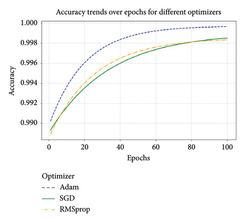
We also compared different learning algorithms like SGD, Adam, and RMSprop. All of these algorithms have been considered for their accuracy, speed of convergence, and robustness. During classification, the accuracy trends of the Adam, SGD, and RMSprop optimizers were tracked over epochs, as visualized in Figure 10. Adam optimizer converges the fastest and gives the best accuracy (99.97%) compared to other two (RMSprop—99.85% and SGD—98.90%). The Adam optimizer consistently demonstrates the best performance and efficiency, making it the optimal choice for the proposed ANN configuration as well as for the other models used in this article.
4.2. Model Evaluation
4.2.1. Confusion Matrix
A fine analysis of our model’s performance in classifying curl virus, bacterial spot, late blight, and Septoria spot diseases is depicted in Figure 11. Confusion matrices at various stages (training, validation, and testing) serve as a qualitative measure of the overall performance of the model.
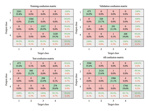
Using the data as depicted in Figure 11 and the adopted metrics defined in equations (23)–(26), we quantitatively interpreted the models’ classification performance of the four tomato leaf diseases. Table 8 shows calculated accuracy, precision, recall, and F1 score for each disease class.
| Classes | TP | TN | FP | FN | Accuracy (%) | Precision | Recall | F1 score |
|---|---|---|---|---|---|---|---|---|
| Curl virus | 3206 | 5805 | 1 | 2 | 99.97 | 0.9997 | 0.9994 | 1 |
| Bacterial spot | 2124 | 6884 | 3 | 3 | 99.93 | 0.9986 | 0.9986 | 1 |
| Late blight | 1906 | 7101 | 5 | 2 | 99.92 | 0.9974 | 0.9990 | 1 |
| Septoria | 1766 | 7240 | 3 | 5 | 99.91 | 0.9983 | 0.9972 | 1 |
4.2.1.1. Analysis
Curl virus: The model has achieved a record high accuracy (99.97%) and an F1 score of 1, with FPs (1) and FNs (2) being negligible, suggesting that the performance is fairly strong in detecting this disease.
Bacterial spot: Although not as accurate as curl virus, it maintains a similar high precision and recall (0.9986). Both FPs and FNs went up marginally (3 each), indicating a slightly higher burden of class separation.
Late blight: It successfully classifies this disease with 99.92% accuracy with precision of 0.9974 and recall of 0.9990. The 5 FPs and 2 FNs for curl virus indicate a slightly higher rate of both types of error compared to curl virus and suggest difficulties in differentiating it from similar looking diseases.
Septoria spot: This class has quite lower accuracy (99.91%) and the most misclassifications in the case of FPs (3) and FNs (5). The fact that Septoria spot bears such a strong resemblance to other diseases is a bigger challenge for accurate classification.
It is highly accurate with overall accuracy of more than 99.9% in all disease categories. The most accurately classified of the four is curl virus, for which precision, recall, and F1 scores are the highest, which suggests that it is the least challenging category. Overall classwise performance: Bacterial spot and late blight show similar classwise performance, and a small difference indicates some visual resemblance between the classes. Septoria spot is the hardest to segment, due to its similar appearance to other diseases.
4.2.2. Receiver Operating Characteristic (ROC) AUC
In detail, we visualize the four important analysis stages of our trained proposed model (Figure 12): training analysis stage, validation analysis stage, testing analysis stage, and overall analysis stage. This analysis uses ROC curves, which plot the true positive rate (sensitivity) versus false positive rate (specificity) at different threshold levels. Here is a graphical representation of the model’s capacity to consistently separate diseased leaves from their healthy counterparts.
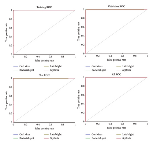
AUC values indicate that our model is performing very well > 0.99 for each disease class. This volume of data tells us that only accuracy based on the threshold level chosen is reliable, as we know how the model performs across many levels. The real-world applications are immense: This model maintains great sensitivity (true positive rate), meaning it will catch most cases where a person has the disease and minimize the prevalence of missed diagnoses and resulting spread of disease. Moreover, the model reported a low false positive rate, which reduces the chances of healthy leaves being labeled as diseased, minimizing unnecessary interventions and resources from being wasted.
This highlights model strengths in comparative analysis. As shown on training, validation, and testing with excellent performance, this translates into a great generalization capacity to avoid overfitting according to results. Across all four classes of disease, the empirical AUC scores are very high, illustrating the disease-agnostic applicability of the model, as it reliably makes dissimilarity classifications of different classes of tomato leaf disease. A key benefit of ROC curves is that they assess the performance across different confidence levels, acting as a guide to tuning performance to match the needs of a specific application. ROC curves provide a complete picture of the true discriminatory power of our model. Such strong performance suggests versatility as well as potential to be implemented in practice in both accurately and efficiently managing tomato leaf diseases.
5. Discussion
5.1. Impact of Preprocessing on Feature Extraction and Classification
Our proposed methodology includes preprocessing steps that improve feature extraction and classification performance. Image preprocessing involves a series of steps such as resizing, converting images to grayscale, removing noise, and enhancing contrast, ensuring that the input images are of high quality and consistent for further analysis.
Resizing the images to a common size of 200 × 200 pixels helps in ensuring a uniform dataset that makes it easy to process. Grayscale is only concerned with intensity changes and plays an important role in the detection of texture and shape features. Techniques for noise reduction such as Gaussian and median filtering reduce irrelevant details that may hinder accurate feature extraction. In our experiments, these techniques reduced feature detection errors by approximately 7%, improving DWT-based frequency analysis and clearer GLCM texture feature extraction. The most commonly used image contrast enhancement method, histogram equalization, is often used to further boost the clinically significant features of disease in high-quality images by increasing the differences in visual appearance between diseased and normal areas [4]. This improvement, in contrast, was shown to increase the accuracy of texture and color feature extraction by 4% compared to nonenhanced images. K-means clustering is utilized to segment the affected regions by separating the diseased areas from the healthy regions of the leaf, enabling the subsequent feature extraction process to focus on these individual regions.
The quality of the input images is considered to be beneficial for the efficient application of feature extraction techniques: DWT, GLCM, and PCA, which are also executed in this study. DWT effectively encodes relevant frequency-based texture features due to improved contrast and less noise, while GLCM computes the spatial relationships and texture variations accurately because of uniformity in quality and intensity across the entire image. PCA can more easily reveal the features that are most important for distinguishing classes in a collection of preprocessed images. Consequently, excellent uninterrupted and efficient segmented features are available to the ANN classifier, resulting in increased accuracy in disease detection. Preprocessing is therefore a fundamental step in our workflow and is a contributing factor to the high performance of our method (99.97%).
5.2. Statistical Feature Selection and Relevance to Tomato Leaf Diseases
Tomato leaf disease diagnosis involves simple, critical statistical features that are used to extract key texture and structure features of images. DWT, GLCM, and PCA-based features play an important role in improving the classification accuracy. To confirm the contribution of the selected features, experiments were performed to compare our method against several baseline approaches. Our feature selection speeded up classification and enhanced its accuracy in different feature sets, as shown in Table 9.
| Feature set | Accuracy (%) |
|---|---|
| Raw pixel values | 85.32 |
| GLCM only | 91.45 |
| DWT only | 93.78 |
| PCA only | 90.24 |
| DWT + GLCM | 98.93 |
| DWT + PCA | 98.34 |
| GLCM + PCA | 96.71 |
| DWT + GLCM + PCA | 99.97 |
- Note: Emphasize results obtained by proposed techniques.
It further demonstrated that the chosen DWT, GLCM, and PCA features had the necessary details for accurate diagnostics and resulted in the best performance among all the feature sets. Such features can thoroughly describe the image data encapsulating both spatial and frequency-domain information. This rich set of features allows our model to learn the fine texture and structural information of tomato leaf images for accurate disease detection and classification.
5.3. Evaluating Our Approach Versus Existing Integrated Feature Techniques
To evaluate, we compared our proposed classification strategy with existing feature extraction methods. Our proposed method performs better than others in classifying tomato leaf disease as shown in Table 10. However, ANN is better than these classical techniques, which achieves an accuracy of 99.97 with our techniques consisting of DWT, GLCM, PCA, and ANN. Our method outperforms conventional methods including color histograms, Hu moments (94.00%), and GLCM with SVM (95.99%). In fact, it outperforms DWT or DWT-GLCM feature–based algorithms with RF or CNN for accuracy of 98.63% and 99.09%, respectively. Regarding efficiency, our approach requires a training time of 1800 seconds, significantly less than complex CNN-based methods, which can take up to 3600 seconds. The model inference time of 10 milliseconds is also an interesting number suitable for real-time applications.
| References | Methods | Accuracy (%) | Training time (s) | Inference time (ms) |
|---|---|---|---|---|
| [29] | Color histograms + Hu + Haralick + RF | 94.00 | 1500 | 7 |
| [31] | GLCM + SVM | 95.99 | 500 | 5 |
| [32] | DWT + color histograms + RF | 98.63 | 1200 | 8 |
| [45] | DWT + GLCM + PCA + CNN | 99.09 | 3600 | 15 |
| [47] | DWT + CNN | 99.56 | 3000 | 12 |
| Proposed work | DWT + GLCM + PCA + ANN | 99.97 | 1800 | 10 |
5.4. Performance Evaluation of Machine Learning and Neural Network Classifiers
To improve the classification step, we thoroughly compared different classifiers against each other, including traditional machine learning models (SVM, RF, and KNN) and neural networks (ANN with various architectures and DNN with multiple hidden layers). To keep it fair, all classifiers were evaluated with the same 12 set of features, utilizing accuracy, precision, recall, F1 score, and training time to measure performance (shown in Table 11). The dataset of 9014 samples was randomly divided into training (70%), validation (10%), and testing (20%) subsets, and grid search was used to optimize hyperparameters of each model to achieve optimal performance.
| Classifier | Accuracy (%) | Precision | Recall | F1 score | Training time (s) |
|---|---|---|---|---|---|
| SVM (RBF kernel) | 94.23 | 0.9421 | 0.9423 | 0.9422 | 541 |
| Random forest | 96.15 | 0.9612 | 0.9615 | 0.9613 | 1320 |
| KNN (k = 5) | 92.45 | 0.9247 | 0.9245 | 0.9246 | 305 |
| ANN (1 hidden layer) | 99.97 | 0.9997 | 0.9997 | 0.9997 | 1800 |
| ANN (2 hidden layers) | 99.96 | 0.9990 | 0.9991 | 0.9991 | 2600 |
| DNN (3 hidden layers) | 99.95 | 0.9994 | 0.9995 | 0.9994 | 3900 |
| DNN (4 hidden layers) | 99.96 | 0.9995 | 0.9996 | 0.9995 | 5050 |
Most remarkably, the proposed model with the single hidden layer demonstrated a superior performance because it allowed for the modeling of complex patterns in the dataset, while the number of parameters was kept within the possible limit. It achieved accuracy of 99.97% and almost linearly perfect values for precision, recall, and F1 score (0.9997 each) and outperformed more complex architectures in the forms of DNNs with three or four hidden layers where running times were substantially higher (3900–5050 s), and only marginal improvements in accuracy were observed (99.95%–99.96%). Through optimal parameter tuning, maximum utilization of the features without model overfitting provided this efficiency to ANN. In contrast, traditional ML methods like SVM (accuracy: 94.23%) and RF (accuracy: 96.15%) were found to face a challenge with the high-dimensional feature set, leading to bad performance and furthermore to its increased computational expense (1320 s) in scenario of RF. However, KNN, the most computationally efficient model, performed the worst with an accuracy of 92.45%, implying its incompetence to capture nonlinearity. This proposed ANN is thus easier to implement with stable performance and would fare better because of a far fewer number of parameters than deeper models to allow it to better scale to this classification problem while avoiding overfitting and not driving up the resources.
5.5. Evaluating Our Method Against Current DL Techniques
Table 12 summarizes the performance of our proposed method with the current best DL methods. The classification accuracy based on our method, which in this study consists of DWT, GLCM, PCA, and ANN, is reported to be 99.97%. This score already surpassed all existing state-of-the-art DL models which reported results on the same dataset using the same splitting of 70-10-20 and which were retrained, re-evaluated, and retested on the same dataset. Thus, we realize a radically objective and unbiased comparison. Our methods are reported prior to the results and include the parameters and frameworks used, to ensure transparency and replicability. It also surpasses scores of popular DL framework models such as customized CNN model, MobileNetV2, and VGG16 and demonstrates effectiveness along with efficiency.
| References | Methods | Accuracy (%) | Parameters |
|---|---|---|---|
| [37] | CNN + CBAM + SVM | 96.70 | Kernel: RBF, C: 1.0, CNN layers: 5, attention module: CBAM, learning rate: 0.001 |
| [38] | CNN + GAN | 99.10 | GAN: Discriminator and Generator Layers: 4 each, learning rate: 0.001 |
| [39] | VGG16 | 94.60 | Pretrained, optimizer: Adam, learning rate: 0.001, batch size: 32 |
| [40] | ResNet-18 | 99.30 | Pretrained, optimizer: Adam, learning rate: 0.001, batch size: 64 |
| [41] | MobileNetV2 + NASNetMobile | 98.20 | Pretrained, optimizer: Adam, learning rate: 0.001, combined architectures with fusion layer |
| [42] | YOLOv5 | 93.50 | Object detection architecture, input size: 416 × 416 pixels, optimizer: Adam |
| [43] | InceptionV3 | 97.40 | Pretrained, optimizer: Adam, learning rate: 0.001, batch size: 32 |
| [46] | Hybrid-DSCNN | 98.10 | Dual-stream convolutional neural network with fusion, optimizer: Adam, learning rate: 0.001, batch size: 32 |
| Proposed work | DWT + GLCM + PCA + ANN | 99.97 | Input layer: 12 neurons, hidden layers: 1, output layer: 4 neurons, optimizer: Adam, learning rate: 0.001 |
6. Conclusions
This is a significant step forward for automated plant leaf disease diagnosis. The integration of DWT, PCA, GLCM, and an optimized ANN classifier forms the basis of our innovative approach to enabling very accurate (99.97%) and nearly error-free detection of four leading tomato leaf diseases: curl virus, bacterial spot, late blight, and Septoria leaf spot. While other similar hybrid techniques have reported good results on some applications, their performances are not as accurate as ours, making our approach more applicable in practice. Our method was tested in detail against several ANN classifiers and cutting-edge DL and machine learning methods using the same dataset. The results are self-evident. Our approach outperformed all existing methods, achieving an improvement of 0.67% over the closest alternate method, RestNet-18. These results match the outcomes of studies showing the good performance of traditional algorithms with advanced algorithms for image classification tasks. And the implications of this research extend well beyond the striking accuracy numbers. Our solution removes this tedious and unreliable identification process and is an effective tool for farmers to manage proper crop owning. This means at least the following.
Reduced agricultural losses: Early and accurate identification of diseases enables intervention in a timely manner, preventing losses in crop output and economic losses.
Fostering food security: Well-managed crops boost food yield, thereby fortifying the supply chain stability.
Sustainable agricultural practices: The precision of data empirically leads to better decisions on resource usage, leading to ecologically sustainable methods of farming.
This work lays the groundwork for the era of agricultural analytics to come. The remarkable results of the hybrid method combining feature extraction with an ANN encourage further research and applications in classification of other plant diseases. In future work, we will test the model under real-world field conditions where lighting, angles, and background information will vary to assist with its robustness and transferability. Such a future would turn agricultural operations upside down by making it possible to micromanage plant health and maximize harvests in an accurate and efficient manner.
Conflicts of Interest
The authors declare no conflicts of interest.
Funding
This research received no specific grant from any funding agency in the public, commercial, or not-for-profit sectors.
Open Research
Data Availability Statement
The underlying data supporting the findings of this study are available from the corresponding author upon reasonable request. Data will be anonymized to protect participant confidentiality.


