In this study, we discuss the approximate solution of the Harry Dym nonlinear partial differential equation and its integrodifferential version. We first construct the Picard successive approximation for the equations under consideration. Then, we give a detailed calculation of the approximate solution for two cases of the partial Harry Dym integrodifferential equation. The approximate solutions are illustrated for some chosen values of the arbitrary constants. The efficiency of this semianalytical method is demonstrated through discussing the regions of the domain with small errors as well as by extracting the exact solution from the limit of the approximation.

1. Introduction

The semianalytical methods have become a popular approach to manipulate both ordinary and partial nonlinear differential equations. The Picard iteration method has been widely used by researchers to calculate the solution, Robin studied the solutions of partial and ordinary differential equations using this iteration method [1], and Bildik introduced comparison study between Picard successive and modified Krasnoselskii iteration to solve the initial value problem of ordinary differential equations [2]. Moreover, the study of Turab utilizes this method to compute the numerical solution of ordinary integrodifferential equations with initial conditions [3].

Lal employed the Picard successive method to solve some problems of nonlinear ordinary differential equations with boundary conditions; their study concluded that this method is accurate and efficient [4]; on the other hand, Yassein presented a study that used an iterative method to solve the ordinary integrodifferential equations in high order, and the solution found was a series that approached the exact solution [5].

Recently, the iteration method has been widely employed to deal with partial differential equations or combine it with some integral transforms, such as the Abdulazeez study, which obtained an analytic solution of a pseudohyperbolic telegraph partial differential equation in fractional order [6]. Also, the Mohammed study solved the nonlinear KdV-type partial differential equation [7].

The Harry Dym equation is a nonlinear partial differential equation in order three, an essential dynamic equation utilized across several physical applications. Mokhtari [8] used Adomian decomposition, variational iteration, and direct integration to generate exact travelling wave solutions to the Harry Dym equation given as

(1)

Ma [9] considered an extended Harry Dym equation. The study of Gonzalez-Gaxiola, Ju, and Ed [10] introduced a new iterative method to obtain an approximate analytical solution to the Harry Dym equation. The study determined that this method was efficient and accurate. Matviichuk [11] dealt with this equation via the theory of finite–dimensional dynamics method, and the exact solution has been obtained. Kumar, Singh, and Kılıçman [12] introduced a study of the nonlinear time fractional Harry Dym equation, which processed the problem in two techniques. Assabaai [13] employed the Lie symmetry group method and Chebyshev spectral method to derive the numerical approximation of the solution of the classical Harry Dym equation (Equation 1), the first was based on the homotopy perturbation method and integral transform, and they used He’s polynomial for the nonlinear part; secondly, they used the Adomian decomposition method to calculate the solution. In their study, they showed that the solutions obtained using the two approaches agreed. Furthermore, Huang and Zhdanov [14] studied the fractional Harry Dym equation with Riemann–Liouville derivative; also, Rawashdeh [15] studied the fractional Harry Dym equation by the fractional reduced differential transform method.

The purpose for studying the integrodifferential equations is that they play an important role in various fields of engineering and science, such as applied mathematics [16], and in general, the majority of initial or boundary value problems that included partial differential equations can be transformed into integral equation problems. Since the integrodifferential equations are typically difficult to solve in analytical method, therefore, in this study, we will use the Picard successive technique to obtain the solution to the nonlinear partial integrodifferential equation, a generalized version of the Harry Dym equation, which is considered novel and different from previous studies mentioned above. This equation is given as

(2)

where f(u) and g(x) are some known functions. We refer to Equation (2) as the Harry Dym partial integrodifferential equation (HDPID). In the case of f = 0 and g = 0 , the above equation becomes the classical Harry Dym partial differential equation (Equation 1). In the following, we construct approximate solutions for Equation (2) using the Picard successive method, and then, we extract the exact solution from the limit of the approximate solution in terms of the Taylor expansion.

2. Picard Successive Method

In this section, we present the Picard successive approximations of the HDPID (Equation 2).

First, consider the initial value problem involving Equation (2) written compactly as

(3)

with the initial condition

(4)

where the right-hand side of Equation (3) is

(5)

Then, by integrating both sides of Equation (3) and Equation (4), we obtain the equivalent integral equation.

(6)

The Picard successive method is employed for Equation (6) to extract iterative approximations of the solution. From the initial condition, we define the first Picard approximation as

(7)

The n^th Picard successive approximation is denoted by u_n(x, t) for which we define the following:

(8)

By substituting Equation (8) in the integral Equation (6), we construct the following formula for the Picard successive approximations:

(9)

Next, we define the n^th order approximate solution

to be the part of the Picard approximation with order of the variable t that is less than n, that is,

where O(tⁿ⁺¹) represents all the terms in Equation (9) with the order of the variable t higher than n. The part O(tⁿ⁺¹) is considered noise terms in the Picard approximation( Equation (9)), and therefore, will be neglected to end up with the n^th approximate solution

of the IVP Equation (3) and Equation (4) calculated as

In fact, as we will show in the next section, the n^th approximate solution

coincides with the Taylor polynomial of degree n for the exact solution which takes the form

Such result induces that the exact solution of the BVP in Equation (3) and Equation (4) can be extracted in the Taylor expansion form from the limit of the approximation as follows:

(10)

3. The Approximate Solution of the Integropartial Differential Equation

The aim of this section is to calculate approximate solutions for the integrodifferential Harry Dym equation using the Picard successive approximations method. We also describe how can the exact solution be extracted from the limit of the approximation. We will consider two cases to define the functions f(u) and g(x) in the HDPDE (Equation 2).

Case 1.

(11)

where a, b, and c are some arbitrary real constants, while A is some combination of a, b, and c.

In the case of A = 0, then, we have f(u) = g(x) = 0 leading to the classic nonlinear Harry Dym equation (Equation 1), which admits the solution (see [8] and [11, 12])

(12)

where

. Otherwise, we define

(13)

Then, the resulted integrodifferential equation (Equation 2) also admits the same solution defined in Equation (12).

For both cases, we consider the initial condition.

(14)

Next, we calculate the Picard successive approximations of the HDPID (Equation 2). Define

(15)

(16)

where μ_n(x, τ) for n > 0 is defined as follows:

(17)

Now, when n = 0

(18)

By substituting Equation (18) into Equation (16), we obtain u₁ as

By neglecting the O(t²) part and comparing the terms in the approximation to the Taylor polynomial of the exact solution in Equation (12), we have

(19)

Next, the μ₁(x, τ) after neglecting the higher terms O(t²) is

(20)

So, the second iteration is

And by comparing to the Taylor polynomial,

(21)

Next, n = 2.

The third approximation is

Also, it can rewrite u₃ as below

(22)

Now, in the same manner, the next successive approximations are calculated as

(23)

(24)

Finally, by continuing this procedure, we obtain the successive approximation u_n which leads in the limit as n⟶∞ to the expansion of the exact solution defined in Equation (11); hence, the exact solution has been obtained.

Case 2. In this case, we define the functions f(u) and g(x) as

(25)

The corresponding HDIPD equation (Equation 2) admits the solution as

(26)

where a, b, c are arbitrary constants. We consider the initial condition

(27)

Now, the Picard successive approximations of the solution are calculated as follows:

(28)

(29)

for n > 0, where μ_n(x, t) is define as

(30)

First, according to the above equation, μ₀ becomes

(31)

Substituting μ₀ into Equation (29) to obtain u₁ as

By neglecting the high-order terms O(t²) and comparing to the Taylor polynomial of the solution in Equation (26), we have

(32)

Next,

after ignoring the terms of high order, then

(33)

So, the second approximation is

(34)

Next,

(35)

Then, the third approximation is

Now, following the same calculation procedure, in the next successive approximations, the higher order terms will vanish since the exact solution itself is a polynomial of Degree 3, yielding to u₄(x, t) = u₅(x, t) ⋯ = u_n(x, t) = T₃[u(x, t)]; therefore, the exact solution is extracted straightforward as

(36)

4. Illustrating Examples

In this section, we introduce two examples of the HDNID (Equation (2)) corresponding to Case 1 and Case 2 of defining the functions f(u) and g(x).

Example 1. In this example, the approximate solution will be calculated for Equation (2) with the case

(37)

(38)

with the constants’ values a = 0, b = −3, c = 3. The initial condition is

(39)

Following the procedure presented in the previous section, the first four approximations have the forms as shown in Table 1.

Table 1. The Picard successive approximations up to order O(t⁴) of the solution of Equation (2) with conditions (Equation (37)) and Equation (38) with initial condition (Equation (39)).

n	The approximate solutions
0
1
2
3
4

Furthermore, it can rewrite the

as below

(40)

Hence, the sequence of the approximations

leads to the Taylor expansion of the exact solution

(41)

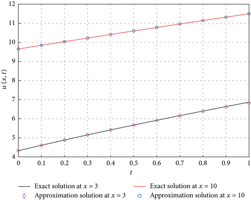
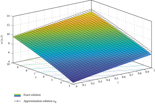
In Figure 1, we present 2D and 3D graphs, for the 4^th approximation plotted against the exact solution. The figures show how close the approximate solution is to the exact solution in the domain 0 ≤ t ≤ 1 and 3 ≤ x ≤ 10, and it shows well approximation of the exact solution in the selected region of the domain. Examples of the numeric values of the exact solution, approximate solution, and the error between them are given in Table 2. The error increases as t increases and x decreases due to the proportion of the approximation terms to the variables t and x.

Details are in the caption following the image — **Figure 1 (a)**
Open in figure viewer PowerPoint

Comparison graphs of the exact and approximate solution for Example 1. (a) 2D graph of the 4^th approximation (dashed line) versus the exact solution (solid line) for x = 3 and x = 10. (b) 3D graph of the 4^th approximation (black mesh) versus the exact solution (colored surface).

Table 2. A comparison of the numeric values of the 4^th approximate solution to the exact solution of Example 1 at x = 10, for discrete values in the interval 0 ≤ t ≤ 1.

n	t	Exact	4^th order	Error
1	0.0	9.6549	9.6549	0.0000
2	0.1	9.8470	9.8470	0.0000
3	0.2	10.0373	10.0373	0.0000
4	0.3	10.2258	10.2258	0.0000
5	0.4	10.4126	10.4126	0.0000
6	0.5	10.5977	10.5977	0.0000
7	0.6	10.7812	10.7812	0.0000
8	0.7	10.9632	10.9631	0.0001
9	0.8	11.1437	11.1436	0.0001
10	0.9	11.3227	11.3225	0.0002
11	1.0	11.5003	11.4999	0.0004

Example 2. In this example, the approximate solution will be calculated for Equation (2) with the case

(42)

(43)

For the constants’ values a = 0, b = 1, c = 1, then the initial condition is

(44)

According to the analysis of Case 2 in the previous section, the approximations of the solution are given as follows (Table 3).

Table 3. The Picard successive approximations up to order O(t⁴) of the solution of Equation (2) with conditions (Equation (37)) and Equation (38) with initial condition (Equation (39)).

n	The approximate solutions
0
1
2
3

As the previous example, it can rewrite the u₃ as below

(45)

It is clear that

; therefore, the limit leads to the exact solution of the form

(46)

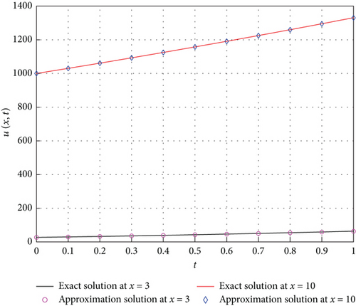
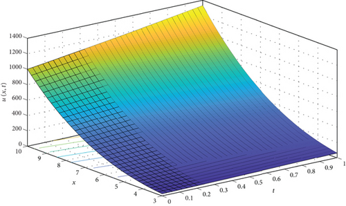
In Figure 2, we present 2D and 3D graphs, for the 2^nd approximation plotted against the exact solution. The figures show how close the approximate solution is to the exact solution in the domain 0 ≤ t ≤ 1 and 0 ≤ x ≤ 10, The figure shows a good approximation of the exact solution in the selected region of the domain. Examples of the numeric values of the exact solution, approximate solution, and the error between them are given in Table 4.

Table 4. A comparison of the numeric values of the 2^nd approximate and 3^rd approximate solution with the exact solution of Example 2 at x = 3, for discrete values in the interval 0 ≤ t ≤ 1.

n	t	Exact	2^nd order	Error 2^nd order	3^rd order
1	0.0	27.000	27.00	0.000	27.000
2	0.1	29.791	29.79	0.001	29.791
3	0.2	32.768	32.76	0.008	32.768
4	0.3	35.937	35.91	0.027	35.937
5	0.4	39.304	39.24	0.064	39.304
6	0.5	42.875	42.75	0.125	42.875
7	0.6	46.656	46.44	0.216	46.656
8	0.7	50.653	50.31	0.343	50.653
9	0.8	54.872	54.36	0.512	54.872
10	0.9	59.319	58.59	0.729	59.319
11	1.0	64.000	63.00	1.000	64.000

5. Discussion

The detailed analysis presented in Section 3 and Section 4 shows that the suggested semianalytic technique is effective to obtain approximate and exact solution of the proposed nonlinear integropartial differential equations. The technique starts with transforming the integropartial differential equation into an integral representation. Then, the approximate solutions derived from the Picard successive method through iterative integration process. The output of this process is polynomials of the variable t with coefficients depending on x. In order to maintain a well representation of the approximation, all terms in the approximation having a power of the variable t higher than the iteration index is considered noise to be neglected. The resulted approximation then can be shown to coincide with the Taylor polynomial of the exact solution in the variable t. Therefore, the exact solution can be induced from the limit of the approximate solution as a Taylor expansion.

Some key issues to mention here are the dependence of the iterative process on the choice of the initial condition to construct successive approximations that lead clearly to the Taylor expansion of the exact solution. An effective way to achieve that is to neglect the high-degree terms in each iteration. Given an appropriate choice of the initial condition, the resulted approximations can be compared directly to the Taylor polynomial of the exact solution. Although the exact solution can be induced from the limit of the iteration as a Taylor expansion, the resulted Taylor power series might not converge on all the domains of the variables t and x.

As described in Case 1 of Section 3 and illustrated in Example 1, the variable t appears in the numerator of the terms in the approximation while the variable x appears in the denominator, except for the first term. Therefore, the terms are directly proportional to t and conversely proportional to x. Hence, the convergence of the resulted approximation is associated with small values of the variable t and large values of the variable x which is to decrease the errors (see Table 2). On the other hand, in Case 2 and Example 2, the resulted Taylor expansion is a polynomial, which converges for all the values of the variables t and x (see Table 4).

6. Conclusion

The nonlinear partial integrodifferential equations, a generalized version of the Harry Dym partial differential equation, are solved by using the Picard successive method, which provides an explicit iterative process to generate The presented analysis shows the effectiveness of the method in extracting the exact solution of the problem given an appropriate choice of the initial condition, and the study concludes that the same traditional solution is obtained when using the same initial condition, however, with variations in the arbitrary constant values. Moreover, when terms that are added to the classical equation vanish under certain conditions, the technique is still effective and gives the results that are mentioned in the literature review.

Furthermore, the study considers different types of cases. The Picard method gives the solution in polynomial form, which tends to be the exact solution.

The limitations of the method have also been presented by discussing the convergence conditions that restrict the values of the independent variables. A detailed description of the process has been included and illustrated with representative examples.

Conflicts of Interest

The author declares no conflicts of interest.

Funding

The author declares that he has no sources of funding (institutional, private, and corporate financial support) for the work reported in his manuscript.

Acknowledgments

This work is supported by the College of Basic Education at the University of Mosul, Iraq.

Open Research

Data Availability Statement

The author confirms that the data supporting the findings of this study are available within the article.

References

1 Robin W., Solving differential equations using modified Picard iteration, International Journal of Mathematical Education in Science and Technology. (2010) 41, no. 5, 649–665, https://doi.org/10.1080/00207391003675182, 2-s2.0-77957878704.
10.1080/00207391003675182
Google Scholar
2 Bildik N., Bakir Y., and Mutlu A., The new modified Ishikawa iteration method for the approximate solution of different types of differential equations, Scientia Iranica. (2013) 2013, no. 1, 1792–1804, https://doi.org/10.1186/1687-1812-2013-52, 2-s2.0-84902506245.
10.1186/1687-1812-2013-52
Google Scholar
3 Turab A., Montoyo A., and Nescolarde-Selva J.-A., Computational and analytical analysis of integral-differential equations for modeling avoidance learning behavior, Journal of Applied Mathematics and Computing. (2024) 70, no. 5, 4423–4439, https://doi.org/10.1007/s12190-024-02130-3.
10.1007/s12190-024-02130-3
Google Scholar
4 Lal M. and Moffatt D., Picard′s successive approximation for non-linear two-point boundary-value problems, Journal of Computational and Applied Mathematics. (1982) 8, no. 4, 233–236, https://doi.org/10.1016/0771-050X(82)90045-6, 2-s2.0-0020248331.
10.1016/0771-050X(82)90045-6
Google Scholar
5 Yassein S. M., Application of iterative method for solving higher order integro-differential equations, Ibn AL-Haitham Journal For Pure and Applied Sciences. (2019) 32, no. 2, 51–61, https://doi.org/10.30526/32.2.2139.
10.30526/32.2.2139
Google Scholar
6 Abdulazeez S. and Modanli M., Analytic solution of fractional order pseudo-hyperbolic telegraph equation using modified double Laplace transform method, International Journal of Mathematics and Computer in Engineering. (2023) 1, no. 1, 105–114, https://doi.org/10.2478/ijmce-2023-0008.
10.2478/ijmce-2023-0008
Google Scholar
7 Mohammed A., Al-Ramadhani S., and Darghoth R., The possible solutions for the two KdV-type equations using a semi-analytical Kamal-iteration method, European Journal of Pure and Applied Mathematics. (2022) 15, no. 4, 1917–1936, https://doi.org/10.29020/nybg.ejpam.v15i4.4599.
10.29020/nybg.ejpam.v15i4.4599
Web of Science® Google Scholar
8 Mokhtari R., Exact solutions of the Harry—Dym equation, Communications in Theoretical Physics. (2011) 55, no. 2, 204–208, https://doi.org/10.1088/0253-6102/55/2/03, 2-s2.0-79951759802.
10.1088/0253-6102/55/2/03
Web of Science® Google Scholar
9 Ma W.-X., An extended Harry Dym hierarchy, Journal of Physics A: Mathematical and Theoretical. (2010) 43, no. 16, article 165202, https://doi.org/10.1088/1751-8113/43/16/165202, 2-s2.0-77950580038.
10.1088/1751-8113/43/16/165202
Google Scholar
10 Gonzalez-Gaxiola O., Ju U. D. C. S., and Ed S. O., Iterative method for constructing analytical solutions to the Harry-DYM initial value problem, International Journal of Applied Mathematics. (2018) 31, no. 4, 627–640, https://doi.org/10.12732/ijam.v31i4.8, 2-s2.0-85052060130.
10.12732/ijam.v31i4.8
Google Scholar
11 Matviichuk R. I., Dynamics and exact solutions of the generalized Harry Dym equation, Proceedings of the International Geometry Center. (2019) 12, no. 4, 50–59.
10.15673/tmgc.v12i4.1682
Google Scholar
12 Kumar D., Singh J., and Kılıçman A., An efficient approach for fractional Harry Dym equation by using Sumudu transform, Abstract and Applied Analysis. (2013) 2013, no. 1, https://doi.org/10.1155/2013/608943, 2-s2.0-84878744502, 608943.
10.1155/2013/608943
Google Scholar
13 Assabaai M., Numerical solution of the Harry Dym equation using Chebyshev spectral method via lie group method, Journal of Physics: Conference Series. (2021) 1900, no. 1, https://doi.org/10.1088/1742-6596/1900/1/012004.
10.1088/1742-6596/1900/1/012004
Google Scholar
14 Huang Q. and Zhdanov R., Symmetries and exact solutions of the time fractional Harry-Dym equation with Riemann–Liouville derivative, Physica A: Statistical Mechanics and its Applications. (2014) 409, 110–118, https://doi.org/10.1016/j.physa.2014.04.043, 2-s2.0-84901029921.
10.1016/j.physa.2014.04.043
Web of Science® Google Scholar
15 Rawashdeh M. S., A new approach to solve the fractional Harry Dym equation using the FRDTM, International Journal of Pure and Applied Mathematics. (2014) 95, no. 4, 553–566, https://doi.org/10.12732/ijpam.v95i4.8, 2-s2.0-84907718769.
10.12732/ijpam.v95i4.8
Google Scholar
16 Kythe P. and Puri P., Computational methods for linear integral equations, 2011, Springer Science \& Business Media.
Google Scholar

All articles

Approximate Solution of an Integrodifferential Equation Generalized by Harry Dym Equation Using the Picard Successive Method

Abstract

1. Introduction

2. Picard Successive Method

3. The Approximate Solution of the Integropartial Differential Equation

4. Illustrating Examples

5. Discussion

6. Conclusion

Conflicts of Interest

Funding

Acknowledgments

Open Research

Data Availability Statement

References

Figures

References

Information

About Wiley Online Library

Help & Support

Opportunities

Connect with Wiley

Approximate Solution of an Integrodifferential Equation Generalized by Harry Dym Equation Using the Picard Successive Method

Abstract

1. Introduction

2. Picard Successive Method

3. The Approximate Solution of the Integropartial Differential Equation

4. Illustrating Examples

5. Discussion

6. Conclusion

Conflicts of Interest

Funding

Acknowledgments

Open Research

Data Availability Statement

References

Figures

References

Related

Information