Ethiopian Traffic Sign Recognition Using Customized Convolutional Neural Networks and Transfer Learning
Abstract
Intelligent transportation systems rely greatly on their capacity to identify and recognize traffic signs. Traffic signs are important for modern transportation systems because they keep roads safe and help drivers, especially in areas like Ethiopia where sign designs are unique and diversified. In this study, we presented a convolutional neural network (CNN)–based model for Ethiopian traffic sign recognition (ETSR) purposes. We applied the transfer learning technique to fine-tune the pretrained models, namely, MobileNet, VGG16, and ResNet50. Both training and model hyperparameters are fine-tuned, and the 11,000 Ethiopian traffic sign images, which have 156 unique signs, are leveraged to build the new models. Optimizer, batch size, learning rate, and epoch are among the tuned training hyperparameters. All convolutional bases (learning layers) are trained using new weights. We built the fully connected layer of each model from two batch normalization layers and two dense layers. The output layer of the models has 156 units (neurons) with a softmax activation layer. The performances of newly developed models are rigorously compared with those of the base (pretrained) models. The best model was also selected after rigorous experiments. Based on the experiment, we achieved testing accuracy of 97.91%, 93.45%, and 80.18% for fine-tuned VGG16, MobileNet, and ResNet50, respectively.
1. Introduction
In one nation’s transportation system, road traffic is very imperative for safety and harmony in the flow of traffic. A road traffic accident (RTA) is an incident on a way or street open to public traffic, resulting in one or more persons being killed or injured, and involving at least one moving vehicle [1–4]. It has become one of the most significant public health problems in the world, claiming over 1.3 million lives and leading to 20 to 50 million serious injuries every year, especially in developing countries because human being’s day-to-day activities are highly correlated with transportation [5–9]. Ethiopia is one of the countries with the worst RTA records in the world, and it ranks second among East African countries [6–8]. In many developing countries, there is a paucity of evidence regarding the epidemiology of RTAs. Data on the magnitude of RTAs were mostly obtained through police records and hospital registration data. However, insufficient data reporting masked the gravity of the problem, and little attention was paid to the magnitude and correlation of RTAs from the driver’s perspective [10–12].
Commonly, placing traffic signs across the road is one way of minimizing accidents because traffic signs provide important information to the drivers about the road and other things in that specific place. But drivers are sometimes insensitive to those signs due to carelessness, lack of attention, and other different reasons. As a consequence, the probability of having an accident goes up with signs left unnoticed and unapplied by drivers. Hence, to resolve this threat of road accidents in this era of technological advancement, different countries are continuously working toward developing different driver assistance systems, like the traffic sign detection and recognition (TSDR) system. The TSDR system plays a vital role in increasing road safety and traffic management systems. With the rapid expansion of road networks and urban development in Ethiopia, there is a growing need for robust and efficient systems to detect and recognize Ethiopian traffic signs. However, building accurate traffic sign recognition (TSR) and detection systems for Ethiopia faces challenges, including the scarcity of annotated datasets tailored to the country’s specific signage and regulatory requirements [13–16].
- •
Ethiopian traffic sign recognition (ETSR) does not have a publicly available dataset. To address this problem, we created the first dataset of Ethiopian traffic signs in this work. As a result, this dataset may be utilized in further research to enhance the intelligent transportation system.
- •
To recognize Ethiopian traffic signs for the first time, we create the new models by fine-tuned pretrained models.
- •
By adding two batch normalization layers to the CNN classifier layer, which minimized overfitting by reducing the amount of complicated computation conducted at the fully connected layer, an efficient traffic sign recognizer model was developed. This feature helped the model to compute an efficient and reliable recognition task, which improved the model’s performance.
- •
The proposed approach has the potential to contribute to the development of intelligent transportation systems tailored to the Ethiopian context, ultimately enhancing road safety and traffic efficiency across the country.
The rest of the work is structured as follows. Section 2 presents a detailed description of the related works. Section 3 provides a detailed description of the proposed methodology and the dataset analyzed in this study. The experimental findings and analyses are provided in Section 4. Finally, we express our concluding remarks in Section 5.
2. Related Works
This section presents a concise description of the numerous kinds of detection and recognition of traffic sign that have been proposed. This field of research has received a lot of attention in recent times, especially with the advent of public-domain intelligence transportation system, and significant efforts and advancements have been made.
In study [17], a new high-performance and robust deep CNN model is proposed for TSR. The model is presented by combining the trained models by applying improvement methods to the input images. Gradient-weighted class activation mapping (Grad-CAM) was used to make the model explainable. The migration test is applied to the Belgium Traffic Sign Classification (BTSC) dataset to test the robustness of the model. With the transfer learning method of the models trained with German Traffic Sign Recognition Benchmark (GTSRB), the parameter weights in the feature extraction stage are preserved, and the training is carried out for the classification stage. However, the parameters of the models trained on a single preprocessed dataset were not trained, and transfer learning was performed. Thus, the number of trainable parameters in the ensemble model is only 39,643.
In work [18], they proposed an improved network LeNet-5 model for the classification of road signs. They trained their model network on the GTSRB database and also on the Belgian Traffic Sign Dataset (BTSD). The lightness and the reduced number of parameters in their model (0.38 million) based on the enhanced LeNet-5 network pushed them to test their model for an embedded application using a webcam. In [19], the authors focused on precisely detecting and recognizing traffic signs that are present on the streets using computer vision and deep learning techniques. For further improvement, models are employed in a multitask learning approach. Hence, different experiments have been carried out using pretrained architectures like Inception, ResNetV2, and DenseNet201. A range of traffic signs and traffic lights are employed to validate the designed model.
The paper [20] presents a comparison between an 8-layer CNN and some state-of-the-art models, such as VGG16 and ResNet50, for traffic sign classification (TSC) on the GTSRB. Their 8-layer model was able to achieve 96% test accuracy. The authors of [21] proposed a CNN-twin support vector machine (TWSVM) hybrid model by fusing the TWSVM with higher computational efficiency as the CNN classifier, and it was applied to the TSR task. To improve the generalization ability of the model, the wavelet kernel function is introduced to deal with the nonlinear classification task. On the GTSRB and BELGIUMTS datasets, the validity and generalization ability of the improved model are verified by comparing it with different kernel functions and different SVM classifiers.
In paper [22], TSR and classification are implemented using the transfer learning concept. They experimented with three pretrained models, like InceptionV3, ResNet50, and Xception. The results from using each of these models are compared in terms of efficiency and accuracy. The transfer learning models are trained using the GTSRB dataset. The paper in [23] presents a comprehensive comparative analysis of five popular transfer learning–based CNN approaches, namely, Xception network, InceptionV3 networks, ResNet50, VGG16, and EfficientNetB0 models, for the recognition of GTSRB traffic signs. The Xception network has been proven to be highly successful in terms of accuracy (95.04%), minimum loss value (0.2311), and affordable speed and training time, whereas ResNet50 and EfficientNetB0 obtained good accuracy with fewer model parameters.
Study [24] provides an experimentation method involving building a CNN model based on a modified LeNet architecture with four convolutional layers, two max-pooling layers, and two dense layers. The model is trained and tested with the GTSRB dataset. The results show that the proposed model achieved 95% model accuracy with an optimum number of epochs. The paper in [25] proposed a novel model called Traffic Sign Yolo (TS-Yolo) based on the CNN to improve the detection and recognition accuracy of traffic signs, especially under low visibility and extremely restricted vision conditions. The experimental results demonstrated that using the YOLOv5 dataset with augmentation, the precision was 71.92, which was increased by 34.56 compared with the data without augmentation.
Reference [26] provides a camera-based TSR system created to assist drivers and self-driving automobiles in overcoming this difficulty. After being trained on a significant amount of data, including synthetic traffic signs and photos from street views, the proposed multitask CNN refines and classifies the data to their precise classifications. In research [27], they examined the application of deep transfer learning to use intelligence gathered from an established, standard dataset of traffic signs from a given country or region and use it to improve the recognition of traffic signs from another country or region using a deep learning framework. They used VGG16 deep transfer learning algorithms and achieved 95.61% accuracy. In paper [28], they implemented an experiment to evaluate the performance of the latest version of YOLOv5 based on their dataset for TSR, which unfolds how the model for visual object recognition in deep learning is suitable for TSR through a comprehensive comparison with a single-shot multibox detector. The experiments in this project utilize their dataset. According to the experimental results, YOLOv5 achieves 97.70%.
In paper [29], they presented a deep learning–based autonomous scheme for the recognition of traffic signs in India. Automatic TSDR was conceived using a CNN and refined mask R-CNN (RM R-CNN)–based end-to-end learning. The proffered concept was appraised via an innovative dataset comprised of 6480 images that constituted 7056 instances of Indian traffic signs grouped into 87 categories. The dataset for training and testing of the proposed model is obtained by capturing images in real time on Indian roads. The evaluation results indicate a lower than 3% error. The study [30] investigated the effectiveness of transfer learning feature-combining models, particularly in classifying traffic signs. The VGG16 and VGG19 TL feature models were combined with two classifiers, random forest (RF) and neural network. From the results obtained, the best pipeline was VGG16+VGG19 with an RF classifier, which was able to yield an average classification accuracy of 0.9838.
In [31], an overview of different traffic sign detection (TSD) and TSC methods was proposed, aiming to choose the best ones in terms of accuracy and processing time. The developed TSC model is trained on the GTSRB dataset and then tested on various categories of road signs. The achieved testing accuracy rate reaches 98.56%. To improve the classification performance, they proposed a new attention-based deep CNN. The achieved results are better than those existing in other TSC studies. In [32], they developed a recognition system that increases the classification accuracy of the model using deep learning methods for road sign recognition for drivers in real time on the road. The proposed road sign recognition system was trained using 43 different road signs, and it can work in real time to recognize the image of road signs.
In this study, recognition of traffic sign using customized CNN models was experimented and analyzed. A comprehensive comparative analysis was also performed among the three fine-tuned and base models to compare the performance with the models such as VGG16, MobileNet, and ResNet50. Finally, the model that best recognizes the Ethiopian traffic sign was selected.
3. Materials and Methods
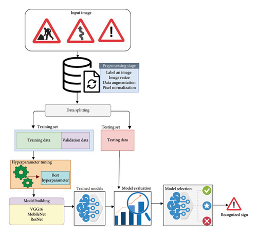
There are some studies that worked on TSR. They used their own methods to come up with the solution. Some built their own custom model while others used the transfer learning technique. We have used a scientific approach to achieve this study. Figure 1 shows the high-level procedure of how this study was handled. Our initial task was collecting traffic sign image data and labeling (annotating) of the image data. At the second phase, we performed image processing. At the third phase, data splitting was carried out. The fourth task of this study included hyperparameter tuning and model training. At the fifth phase, we used different evaluation metrics to evaluate the recognition performance of the models. Finally, we selected the best model.
3.1. Dataset
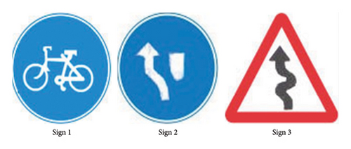
We used locally collected Ethiopian traffic sign images for the purposes of our study. We went over with a driver license trainer with five years of experience on exactly how to annotate these data after we immediately obtained them from the designated driving license school. Table 1 shows sample annotation method using CSV file. 11,000 Ethiopian traffic sign images with 156 unique categories (classes) were used to achieve the goal. The Ethiopian traffic sign image data have four main categories such as compulsory, information, regulatory, and warning signs. Except in warning signs, 80 images are there for each class in all three sign families. In warning sign, the amount of data for each class is 70. To reduce the model biases due to the dataset, we used data augmentation to overcome environmental variability such as variety of light. We used image data generator, a Keras class for data augmentation. The principal variables used in augmentation techniques are fill mode, brightness range, zoom range, width shift range, height shift range, and horizontal flip. Width and height were shifted to 20% of the image’s width and height to account for positional variability and image deformation. We performed zoom-in and zoom-out operation with 20% of the original zoom status. The brightness range was adjusted in between 0.15 and 2 to reduce model bias due to environmental variability. Nearest fill mode was used to replace missing values when transformations caused pixels to fall outside the image boundaries. This nearest fill mode can replace missing values by replicating the nearest pixel value. We used the three traffic signs as shown in Figure 2 which depicts how we annotated the data displayed in Table 1.
| Sign | Tag | ለብስክሌት_ብቻ_የተፈቀደ_ነው | የአደባባዩን_ግራ_ይዘህ_ንዳ | ዝግዛግ_መንገድ |
|---|---|---|---|---|
| Sign1 | [‘ለብስክሌት_ብቻ_የተፈቀደ_ነው’] | 1 | 0 | 0 |
| Sign2 | [‘የአደባባዩን_ግራ_ይዘህ_ንዳ’] | 0 | 1 | 0 |
| Sign3 | [‘ዝግዛግ_መንገድ’] | 0 | 0 | 1 |
3.2. Data Preprocessing
The study’s image processing phase included concatenating raw images, labeling, data augmentation, image pixel normalization, and image size reduction. In light of the fact that we employed a free GPU and 12 GB of RAM from Google Colaboratory, we encountered session crashes. We are currently obligated to start over the data processing stage initially. The preparation of the data requires a long time. In order to minimize data loading and processing time, we saved the preprocessed data in a single .npy file format. It is evident that a lightweight distribution of pixel values between 0 and 255 produces a colored image. Training may be delayed down by large values of colored image pixels. Consequently, we reduced the size of these large pixel values from 0 to 1. Image resizing means resizing the image to a standard resolution that works with the trained model. Even though the standard input size of the pretrained models used in this study is 224 × 244, we resized the image shape to 64 × 64. This shape reduction helps us preserve the computational resources and the time taken for preprocessing and training.
3.3. Data Splitting
We employed data splitting concepts of 80 by 20. Thereby, training and testing data represent 80% and 20% of the total data, respectively. To put it another way, 2200 data are used to test the models and 8800 data are employed for training. Furthermore, during each training epoch, 20% of the training data are split for validation data, which is used to evaluate the model even though it is still in the learning stage.
3.4. Hyperparameter Selection
Training hyperparameters including learning rate, batch size, and optimizer selection were addressed in the hyperparameter tuning step. In addition, we modified the model’s parameters mainly by applying batch normalization layers at the pretrained model’s fully connected layer and training all convolutional base layers with new weights. While using Google as a resource, we were still limited by computational resources. Because of this, we are unable to use a greedy method to choose the most suitable parameters for training the model. So we attempted the trial-and-error approach. We were able to determine the optimal values for the optimizer, learning rate, and batch size with the values 32, 1 × 10⁻⁴, and Ada-max by Adamax, respectively.
3.5. Model Building
Training deep learning model is effortful and time-consuming. Deep learning needs huge dataset to get amenable recognition performance. Training this deep learning model from scratch requires high performance computer particularly GPU-operated machine, longer training epochs, and massive data. So, to alleviate these resources and data requirements, we employed transfer learning techniques and we fine-tuned the pretrained models. We selected the pretrained models that have been trained on ImageNet (a large-scale dataset) such as MobileNet, VGG16, and ResNet50. ImageNet is a data repository that has millions of image data labeled with 1000 classes.
We used the built-in Keras functions to load these models with pretrained weights. The models are built using CNN that is the backbone of deep learning for image recognition and object detection. Using this CNN, the models are able to extract unique features of traffic sign images automatically while it is on learning. CNN makes the model effectively learn discriminative features from traffic sign images, enabling precise classification. The model’s ability to automatically extract relevant features from complex image data is a significant advantage over traditional methods.
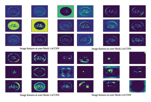
Figure 3 shows how CNN extracts unique features from input image data. At the beginning layer, CNN extracts a very simple structure of an image such as vertical and horizontal lines. At the second layer, CNN starts to identify differently corners, curves, and shapes from the images. Starting from the third layer, CNN applies its power on extracting ubiquitous shapes and structures of the images.
3.5.1. Model Customization (Fine-Tuning)
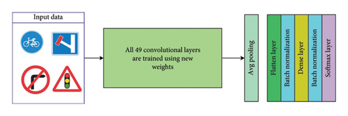
Figures 4, 5, and 6 show the architecture of MobileNet, VGG16, and ResNet50 that we built, respectively. As shown in each figure, we made all convolutional base (feature learning) layers of all models learned using new weights. We removed the original fully connected layer of each pretrained model and used our new layers. Hence, we used two batch normalization layers, one intermediate dense layer and another last dense layer with softmax activation function at the output layers of the models. Since the models are designed for multiclass classification, we used the loss function of categorical cross-entropy.


3.6. Model Evaluation
3.7. Experimental Setup
We leveraged a free 12 GB RAM and GPU from Google Colab to handle the tasks presented from data loading up to model evaluation. First, we augmented our data using Anaconda Navigator. Second, we labeled (annotate) the data in CSV file format. Then we uploaded both image data and CSV file on Google drive. Afterward, we mounted the Google drive to Google Colab to access the uploaded image data and CSV file. After mounting the Google drive, required TensorFlow and Keras libraries are imported. The next step was loading CSV on Colab working environment and preprocessing the data by concatenating the target label with the image data. This concatenation was achieved by matching the file name found in CSV file with the file name of the real image data. The preprocessed data are then saved using a single file name with file format of .npy and loaded to be splite into 80% by 20% for training and testing dataset, respectively. Furthermore, from 80% of training data, 20% of it was split for the validation set. By applying the transfer learning technique, we adjusted various training hyperparameters and model hyperparameters. We used 32, 0.0001, and Ada-max for batch size, learning rate, and optimizer, respectively. All learning layers of the adopted model are trained using new weights. Two batch normalization layers are leveraged at fully connected layer of all pretrained models. Precession, recall, and F1-Score are the basic metrics utilized for model performance evaluation measurement. The type of pretrained model and selected hyperparameters are used as evaluation benchmarks.
4. Result and Discussion
Many rigorous experiments are performed on base models and newly tuned models based on the above experimental setup in Section 3.7, to come up with the best solution. In this section, we only discussed about the results that are attained using the selected best hyperparameters. These hyperparameters are 1 × 10⁻⁴, 32, and Ada-max for learning rate, batch size, and optimizer, respectively. Using these parameters, we conducted a comprehensive performance comparison between base models and fine-tuned (MobileNet, VGG16, and ResNet50) models built by the transfer learning technique.
4.1. Training and Testing Accuracy
Figures 7, 8, and 9 show the training and testing accuracy and loss of VGG16, MobileNet, and ResNet50, respectively. The figure illustrates how the training accuracy and testing accuracy grow up exponentially in a specified training step (epoch). The right side of each figure shows how training and testing loss dropped down with each training step. The left side of each figure shows that the test accuracy of tuned model (our model) was reached at the pick value before the base model. Our fine-tuned models are pretrained by ImageNet data that contain the common traffic sign images. That means the new fine-tuned models did not require learning from scratch to understand (compute) the communally known structures of the traffic signs. This behavior made the fine-tuned models reach their maximum accuracy level before base models. This reveals the ability to generalize better from the test data in less iteration. Likewise, the testing loss values of all fine-tuned model indicated at the right side of the figure degraded down to lowest minima before base model starts from small value of loss.
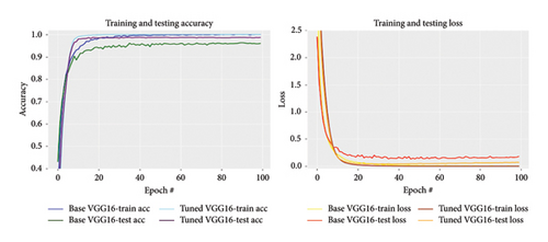
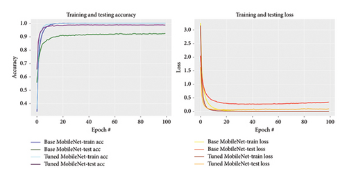
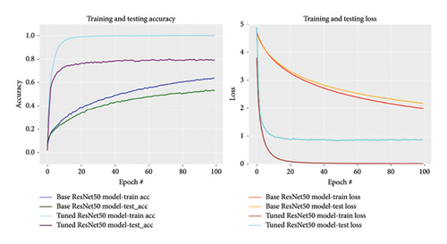
The main purpose of this study was making a comprehensive comparison among three base and fine-tuned models and finally selecting the best one that has improved recognition performance. So, Tables 2 and 3 show the training and testing accuracy of the fine-tuned models. Based on this experiment, the fine-tuned VGG16 model was selected due to its enhanced testing accuracy. The fine-tuned VGG16 model excelled in capturing both complex and high-level features due to its optimally deep architecture, while ResNet shows overfitting behavior due to its very deeper architecture.
| Models | Training accuracy | Testing accuracy |
|---|---|---|
| VGG16 | 99.49 | 97.91 |
| MobileNet | 98.82 | 93.45 |
| ResNet | 95.65 | 80.18 |
- Note: Bold values indicates that maximum accuracy of fine tuned model.
| Models | Training accuracy | Testing accuracy | ||
|---|---|---|---|---|
| Fine-tuned model | Base model | Fine-tuned model | Base model | |
| VGG16 | 99.49 | 99.19 | 97.91 | 96.64 |
| MobileNet | 98.82 | 98.47 | 93.45 | 91.59 |
| ResNet50 | 94.4 | 78.37 | 80.18 | 74.18 |
- Note: Bold values indicates the maximum training accuracy and testing Accuracy of fine tuned and base models based on VGG16.
Generally, in Tables 2 and 3, the fine-tuned models showed amenable improvements over the base models. These enhancements are achieved by the presence of batch normalization at the fully connected layer of the new models. Most CNN models have batch normalization layer at convolutional base (feature learning) layer to reduce the covariant shift. Covariant shift is the change in the distributions of input data to the feature extraction layers. As a result, the layers are forced to adapt this new distribution continuously because the input that the network has learned from forward path is different from the changed input distribution. However, other factors may contribute to accuracy reduction and training time consumption beyond covariance shift. For example, internal covariant shift at fully connected layer is also the main reason for model overfitting. This problem occurred due to computation of a large number of parameters at fully connected layer that has no batch normalization layer.
4.2. Statistical Significance of Testing Accuracy
Table 4 illustrates different testing accuracies of the three models while tested using different optimizers and learning rates. As shown in the table, we used learning rate value of 1∗10−4 and 1∗10−4, and for optimizer, we used Ada-max and Adam. Using smaller batch sizes (4, 8, and 16) can save computational memory, but it needs larger value of epochs and smaller value of learning rate that make the model needing very long time to converge to its optimum accuracy. Unlike smaller batch size, larger batch size needs huge capacity of memory. Hence, we used an optimum batch size (32) for this study.
| Fine-tuned models | Optimizers | |||
|---|---|---|---|---|
| Ada-max | Adam | |||
| Learning rate = 10−4 | Learning rate = 10−5 | Learning rate = 10−4 | Learning rate = 10−5 | |
| VGG16 | 97.18 | 97.91 | 97.55 | 96.05 |
| MobileNet | 90.73 | 93.45 | 92.55 | 93.00 |
| ResNet50 | 74.18 | 80.18 | 79.31 | 86.39 |
Based on these testing accuracies of each fine-tuned model, we analyzed whether the difference in testing accuracy between the models is statistically significant or not using the analysis of variance (ANOVA) algorithm So, the “p” value of 5.78589∗10−5 was achieved which reveals that the difference in testing accuracy between the models is statistically significant. The “p” value (< 0.05 or ≥ 0.05) quantifies the probability that the observed differences in group occurred by random chance, under the null hypothesis. p value < 0.05 means that there is significant difference in testing accuracy.
4.3. Performance Evaluation
It is essential to make a comprehensive evaluation of three fine-tuned models and base model. To evaluate both base model and new models, we importantly used multiple evaluation metrics such as precision, recall, and F1-Score as shown in Table 5. Confusion matrix is also a good model performance analysis method. But the amount of categories in the dataset hindered us to leverage the confusion matrix. So, we only select the best model, and classification reports are used to show the performance of the selected model in each individual class.
| Metrics averaging techniques | Tuned model | Base model | ||||
|---|---|---|---|---|---|---|
| Precision | Recall | F1-Score | Precision | Recall | F1-Score | |
| Macro | 97.69 | 97.78 | 97.68 | 96.45 | 96.36 | 96.28 |
| Micro | 97.91 | 97.91 | 97.91 | 96.64 | 96.64 | 96.64 |
| Weighted average | 97.97 | 97.91 | 97.89 | 96.79 | 96.64 | 96.61 |
Figure 10 shows the F1-Score result of the newly fine-tuned and base models. The figure gives an insight that the fine-tuned model especially VGG16 outperforms the base models to learn from 11,000 traffic sign image data. The classes in our dataset have imbalanced number of samples in each class. So, to reduce biases, F1-Score was the better evaluation metric due to its ability to balance precision and recall by calculating the harmonic mean of them. Hence, this metric was used as benchmark for the comprehensive model performance comparison and we made a conclusion based on this metric.
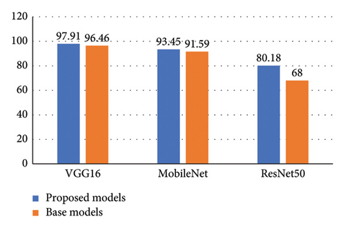
In the multiclass classification technique, classification report particularly recall’s value represents the diagonal values of the confusion matrix. That diagonal values are the correctly classified or true positive (TP) values of the individual class or category incorporated in the dataset. There are 156 categories in Ethiopian traffic sign dataset that are not possible to plot the confusion matrix. So, we only tried to show some categories to save the space in Figure 11. Figure 11 shows the classification report taken from the best fine-tuned model VGG16. The three dot signs in each column indicate that there are omitted classes in between. The values under support column are the amount of testing data in each sample and 2200 is the total testing data splinted from 11,000 traffic sign image data.
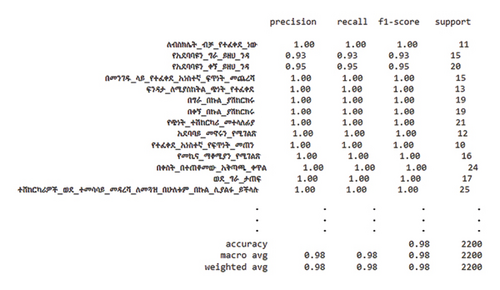
For example, let us take the class “ለብስክሌት_ብቻ_የተፈቀደ_ነው” (bicycle allowed only) and “የአደባብዩን_ግራ_ይዘህ ንዳ” (drive left of the round) by observing the recall values. We selected this value to represent the TP value that could be displayed diagonally at the confusion matrix plot. “ልብስክሌት_ብቻ_የተፈቀደ_ነው” has a recall value of 1. That means 100% of the category are correctly recognized by the model without any misclassification. “የአደባብዩን_ግራ_ይዘህ ንዳ” (drive left of the round) has a recall value of 0.93 which means that 93% of the data are correctly recognized by the model. The remaining 7% of the data are misclassified under other classes or samples. The comparison made in Table 6 illustrates that our work enhances the recognition performance of a model when compared with existing studies.
| Article references | Dataset | Task | Model | No. of classes | Model performance |
|---|---|---|---|---|---|
| [21] | GTSRB | Recognition | CNN | 43 | 96.7 |
| [22] | GTSRB | Recognition | InceptionV3 | 43 | 97.15 |
| [25] | Tsinghua-Tencent 100k | Detection and recognition | YOLOv5 | 220 | 83.73 |
| [27] | GTSRB | Detection and recognition | VGG16 | 43 | 95.61 |
| [28] | Collected | Recognition | YOLOv5 | 43 | 90.14 |
| [29] | ITSD | Detection and recognition | CNN | 87 | 97.08 |
| Proposed model | Collected | Recognition | VGG16 | 156 | Base model (96.46) |
| VGG16 | 156 | Fine-tuned (97.91) | |||
| MobileNet | 156 | Base model (91.59) | |||
| MobileNet | 156 | Fine-tuned (93.45) |
- Note: Bold value indicates that maximum value of model performance and number of classes that we have used in our proposed model.
5. Conclusion and Future Works
5.1. Conclusion
In this study, we carried out a rigorous experiment to recognize 11,000 Ethiopian traffic sign images for the first time. We made an experiment on both fine-tuned and base models of the three pretrained models. The potential of transfer learning and CNN-based model is demonstrated for accurate and efficient identification of the traffic signs. We observed that the fine-tuned model effectively learned from discriminative features of traffic sign images and achieved an accuracy of 97.91, 93.45, and 80.18 for VGG16, MobileNet, and ResNet50, respectively, in classifying 156 traffic sign categories. A comprehensive comparison was performed between the base model and fine-tuned model to analyze the effectiveness of the designed models. As a result, the new model especially VGG16 achieved higher performance than others with F1-Score value of 98%. Another novel feature of this study was the presence of two batch normalization layers at fully connected layer of the CNN model. This novel approach made the model perform agile computation to identify the traffic sign effectively.
5.2. Future Work
Currently, we have developed an optimized model capable of recognizing traffic signs in Ethiopia. We obtained an image of an Ethiopian traffic sign from a driving school and enhanced it to gain a variety of data in terms of color, lightness, and vertical and horizontal alignments. However, extending the dataset’s diversity even more by recording different environmental circumstances will improve the model’s adaptability and applicability. Furthermore, there is a great chance that the Ethiopian traffic sign will be correctly recognized if the output features of two CNN models are combined at the classification layers. A comparative analysis of Ethiopian and other traffic sign datasets may provide an insight for cross-domain challenges. The model’s effectiveness will be increased by future development and integration with mobile applications, which will make it an invaluable resource for students and driving licensing schools everywhere.
Ethics Statement
This research exclusively focuses on the investigation and analysis of Ethiopian traffic sign recognition, with no involvement in experimentation on human subjects, animals, or other subjects.
Conflicts of Interest
The authors declare no conflicts of interest.
Author Contributions
Amlakie Aschale Alemu: data curation, analysis, and interpretation, visualization, methodology, writing, reviewing and editing, and validation.
Misganaw Aguate Widneh: conceptualization, model building and testing, visualization, and document correction.
Funding
No funding was received for this research.
Open Research
Data Availability Statement
The data that support the findings of this study are available from the corresponding author upon reasonable request.


