Research on Small Target Detection Algorithm for Autonomous Vehicle Scenarios
Abstract
In recent years, road traffic object detection has gained prominence in areas such as traffic monitoring, autonomous driving, and road safety. Nonetheless, existing algorithms offer room for improvement, particularly when detecting distant or inherently small targets, such as vehicles and pedestrians, from camera perspectives. By addressing the detection accuracy issues associated with small targets, this study introduces the YOLOv5s-LGC detection algorithm. This model incorporates a multiscale feature fusion network and leverages the lightweight GhostNet module to reduce model parameters. Furthermore, the GC attention module is employed to mitigate background interference, thereby enhancing the average detection accuracy across all categories. Through data analysis, target detection at different scales and sampling rates is determined. Experiments indicate that the YOLOv5s-LGC model surpasses the baseline YOLOv5s in detection accuracy on the Partial_BDD100K and KITTI datasets by 3.3% and 1.6%, respectively. This improvement in locating and classifying small targets presents a novel approach for applying object detection algorithms in road traffic scenarios.
1. Introduction
The rapid advancement in technology and enhancement in hardware capabilities have markedly increased the interest in deploying deep learning technologies within the transportation sector. Notably, applications such as automatic license plate recognition, station facial recognition, vehicle detection and tracking, and pedestrian re-identification have significantly enhanced daily convenience, underscoring the relevance and demand for practical research in this area [1, 2]. Presently, deep learning models are employed to perform comprehensive analyses of traffic-related imagery, including traffic signs, vehicles, and pedestrians, on roadways. This facilitates the accurate detection and recognition of objects within images, thereby aiding decision-making processes and potentially mitigating traffic accidents by enhancing driving assistance mechanisms [3–6].
The application of image object detection technology is extensively recognized across various fields. Nonetheless, its deployment in complex road environments frequently encounters challenges, particularly with the detection of small target objects within images, which can lead to inaccuracies. This issue has contributed to skepticism regarding the reliability of environmental perception technology in autonomous driving systems, especially following traffic incidents attributed to these systems. A significant concern is that certain algorithms exhibit insufficient detection accuracy for small objects. In scenarios where vehicles operate at high speeds and encounter substantial variations, the inability to promptly detect and make informed decisions poses considerable safety risks.
The challenge of effectively detecting small objects persists as a significant hurdle in image analysis. “Small objects” are defined as those entities within an image that either occupy a minimal portion of the space or possess an inherently low pixel count, characterized by limited pixel occupancy, small coverage area, and subtle features, complicating their distinction from surrounding entities. The definition of what constitutes a small object varies, generally bifurcated into two approaches: pixel occupancy and absolute size.
For the pixel occupancy method, an object in an image with a resolution of 256 × 256 is deemed small if its area is under 80 pixels, constituting less than 0.12% of the total area of the image. The absolute size criterion, however, differs across datasets to accommodate inherent size variations. For example, in the COCO dataset, objects are classified based on size: small objects are under 32 × 32 pixels, medium objects fall within 32 × 32 to 96 × 96 pixels, and large objects exceed 96 × 96 pixels. In the CityPersons [7] pedestrian dataset, objects smaller than 75 pixels are considered small. Within urban traffic management datasets, pedestrians and nonmotorized vehicle drivers represented by 30–60 pixels with an occlusion rate below 40% qualify as small objects. Remote sensing and face detection datasets often label entities with 10–50 pixels as small objects. Consequently, a universal definition of small objects in imagery is elusive, heavily depending on the specific detection task and dataset employed.
Many researchers are optimizing classical algorithms to enhance the detection outcomes of small targets. Addressing the intricacies of small target detection involves several innovative strategies, including loss function optimization, multiscale learning, contextual information fusion, and generative adversarial learning. Multiscale learning leverages image pyramids to capture information across various receptive field sizes, facilitating the detection of targets at differing scales. Notably, Jeong et al. [8] introduced the R-SSD model, employing feature fusion across different hierarchical levels to bolster small target detection. Qi et al. [9] proposed an adaptive spatial parallel convolution module (ASPConv), which adaptively gathers corresponding spatial information through multiscale receptive fields to enhance feature extraction capability. Addressing insufficient fusion of semantic and spatial information, they introduced a rapid multiscale fusion module (FMF) to unify the network’s extraction of multiscale feature map resolutions, effectively enhancing small object detection capabilities. Lim et al. [10] enhanced the SSD algorithm by integrating contextual information and an attention mechanism for improved performance. Zhan et al. [11] developed the FA-SSD, which augments the SSD framework with a deep-to-shallow reverse path and a self-attention mechanism to merge adjacent shallow features with up-sampled feature maps, thus enriching shallow semantic information. Liu et al. [12] advanced the capabilities of the YOLOv4 architecture through the YOLOv4-MT network, utilizing feature fusion techniques to elevate detection efficacy. Furthermore, Li et al. [13] applied modifications to the YOLOv5s and CenterNet models specifically for pedestrian target detection. Furthermore, learning contextual information that connects small objects to their surrounding environment significantly improves detection effectiveness. For instance, Li et al. [14] introduced a novel global and local (GAL) attention mechanism that combines fine-grained local feature analysis with global context processing. The local attention focuses on identifying complex details within the image, while the global attention handles broader contextual information. This fusion mechanism allows the model to simultaneously consider both aspects, enhancing overall performance in small object detection. In addition, generative adversarial learning enhances small object semantic information primarily by reconstructing small object feature maps. Some researchers have also improved small object detection by increasing anchor boxes and using model cascades. However, these methods often come at the cost of substantial computational resources. Therefore, to achieve road traffic target detection tasks, this paper does not employ generative adversarial networks to enhance the dataset, increase anchor boxes, or use model cascades. Instead, it adopts multiscale feature fusion and considers global attention mechanisms to maintain a certain detection speed while slightly increasing computational load.
The principal objective of model lightweighting lies in minimizing model size to facilitate deployment in resource-constrained environments and enhance operational speed. This aim has spurred the development of several innovative modules, such as MobileNet and EfficientNet, designed to trim model capacity without substantially compromising performance. Chen et al. [15] unveiled a streamlined network, DCNN, rooted in the DenseLightNet framework, aiming to curtail resource usage and accelerate execution speed. Bie et al. [16] introduced the YOLOv5n network, a real-time, lightweight solution tailored for vehicle detection within a segment of the BDD100K dataset, by integrating depthwise separable convolution with C3Ghost modules. Gu et al. [17] melded MobileNet with feature fusion and a reassignment module into YOLOv4, achieving an adept balance between detection efficacy and deployment simplicity. This configuration reached an average precision of 80.7% on the GTSDB dataset, with detection speeds peaking at 57 frames per second (FPS). Yuan et al. [18] developed YOLOv5s-A2, emphasizing rapid detection and model compactness at the slight expense of accuracy, thereby accommodating the demands of real-time applications and devices with limited computational resources. Junos et al. [19] refined the network architecture by employing mobile inverted bottleneck modules, enhancing the spatial pyramid pooling, and incorporating feature scale layers, culminating in a lightweight model adept at detecting small targets. Meanwhile, Zhu et al. [20] innovatively proposed a lightweight MTNet, which consists of a multidimensional adaptive feature extraction block (MAFEB) and a lightweight feature fusion block (LFFB). MAFEB uses a parallel strategy to integrate it with the attention mechanism, enhancing network performance. LFFB reduces redundant feature map calculations, lowering computational complexity and memory access while maintaining accuracy. This improves channel information interaction and offers a novel approach for small object detection in lightweight networks.
- •
Comprehensive Analysis and Data Label Conversion for Small Road Traffic Targets: We conducted an in-depth analysis of the sizes of road traffic targets in the BDD100K and KITTI datasets. We evaluated the down-sampling results at different magnifications, identified the target sizes and proportions in different datasets, defined the size range for small targets in each dataset, and implemented precise data label conversion. This targeted analysis and processing enhance the accuracy and reliability of small object detection.
- •
Innovative Feature Layer Integration and Lightweight Model Neck Improvements: To address the challenges in small object detection, we introduce additional feature layers specifically dedicated to target detection in the network neck. We propose innovative modifications to the conventional convolutional layers and C3 modules by integrating Ghost convolution and C3Ghost modules. This novel approach significantly reduces the overall model parameters while enhancing detection performance.
- •
Introduction of the C3GC Attention Mechanism: To further improve detection accuracy and mitigate background interference, we introduce a novel global context attention mechanism, the C3GC attention mechanism, into the network backbone. This attention mechanism possesses the powerful ability of nonlocal blocks to model long-range dependencies to enhance overall accuracy in detecting small objects.
These contributions represent a significant advancement in the field of small object detection. Our innovative solutions not only improve detection accuracy but also optimize model efficiency, making them highly suitable for real-world applications in resource-constrained environments. The combination of comprehensive data analysis, novel feature integration, and advanced attention mechanisms underscores the novelty and practical impact of our proposed approach.
2. The Principle of YOLOv5 Algorithm
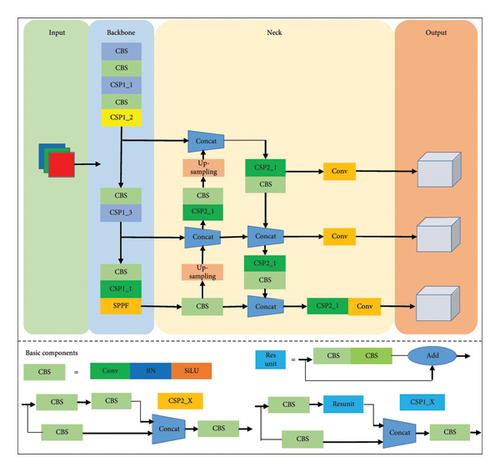
YOLOv5 is a single-stage detection algorithm consisting of several components, including input, backbone network, neck, and output. The backbone network is responsible for feature extraction from input images, the neck is used for fusing the multiscale features extracted by the backbone network, and the output is responsible for generating predictions based on the fused features [21]. Figure 1 illustrates the network structure.
This study leverages the YOLOv5s-6.0 architecture and introduces a tripartite methodology at the input phase to enhance object detection performance: mosaic data augmentation, adaptive image scaling, and adaptive anchor box computation. The mosaic data augmentation technique amalgamates four arbitrarily chosen images through scaling, splicing, and stacking, thereby diversifying the contextual backdrop for object detection. Adaptive image scaling shrinks the image proportionally and applies pixel padding to the nonconforming dimension, ensuring that each side is divisible by the receptive field. This approach minimizes information loss and improves detection speed. Finally, the adaptive anchor box computation iteratively refines anchor box dimensions by comparing them against actual object sizes in the dataset, optimizing for the most precise bounding box predictions. This comprehensive approach not only enriches the input data quality but also fine-tunes the model’s ability to accurately localize and identify objects within varied environments.
The backbone network utilizes a synergistic integration of Conv, CBS, C3, and SPPF modules to adeptly mine deep features pivotal for the detection of small objects. The CBS module, embodying standard convolution alongside batch normalization and SiLu activation, facilitates initial feature extraction. Concurrently, the C3 module, enriched with three conventional convolutional blocks and an array of residual modules, introduces an advanced CSP structure [22]. This structure bifurcates the input channels into dual pathways: one executing standard convolutions and the other deploying residual frameworks for feature amalgamation. The ensuing feature concatenation from both branches fortifies the CSP module, enhancing feature representation.
Further, the SPPF module, an iteration over the seminal SPP, substitutes expansive pooling kernels with multiple diminutive ones. This alteration not only accelerates computational speed but also broadens the feature map, enriching the model’s feature extraction capabilities.
Within the neck layer for feature fusion, YOLOv5 amalgamates the virtues of the feature pyramid network (FPN) and the path aggregation network (PAN), orchestrating a multitiered fusion of features [23, 24]. This fusion stratagem is pivotal for capturing and integrating hierarchical feature representations across different scales, thereby enhancing the model’s sensitivity to object scale variations.
In the terminal phase of output generation, YOLOv5 uses a multiscale detection method to predict the categories and positions of objects of various sizes at three different scales. The computation of bounding box loss leverages the GIOU loss function, while classification and confidence losses are quantified via binary cross-entropy. To refine the precision of detected objects, redundant bounding boxes are culled using nonmaximum suppression (NMS) [25], ensuring the retention of the most salient detections.
3. Algorithm Improvement
3.1. Addition of Shallow Feature Layer
Deep neural networks are celebrated for their expansive receptive fields, which endow them with the capacity to provide rich semantic information. However, this can also lead to the loss of detail information in small targets. Because small targets account for a considerable proportion in some scenarios, this may cause problems in road traffic detection. In contrast, shallow networks, characterized by their constricted receptive fields, are adept at preserving locational data and delivering granular detail, making them inherently more adept at discerning densely situated small targets [26]. To reconcile the need for both comprehensive semantic understanding and precise localization, the integration of a shallow feature layer within the model’s neck is proposed. This strategy leverages the path aggregation feature pyramid network (PAFPN) architecture for effective feature fusion, thereby augmenting the model’s proficiency in small target detection. The resultant enhancement in the detection capability not only ameliorates the model’s sensitivity towards small targets but also substantially elevates the overall accuracy of detection.
Most networks use FPN to implement feature fusion at three scales, which first obtain features down-sampling by eight, sixteen, and thirty-two times of the backbone network and save them as {P3, P4, P5}. Then, P5 features are up-sampled from bottom to top and fused with P4 and P3. Feature fusion at these three scales can achieve detection of some small targets, but it does not simultaneously consider the deep and rich semantic information and shallow detail information; therefore, there is still room for further improvement. This paper modifies the model neck by fusing feature information from four scales, generating four 3D tensors. The value of each tensor is equal to the product of the number of grid units and the predicted categories, anchor box positions, and confidence. Table 1 shows the resolution mapped to different feature layers.
| Resolution | Feature layer | |||
|---|---|---|---|---|
| P2/4 | P3/8 | P4/16 | P5/32 | |
| 16 × 16 | 4 × 4 | 2 × 2 | 1 × 1 | 0.5 × 0.5 |
| 32 × 32 | 8 × 8 | 4 × 4 | 2 × 2 | 1 × 1 |
| 96 × 96 | 24 × 24 | 12 × 12 | 6 × 6 | 3 × 3 |
The effective pixel information gradually decreases as the convolutional layer depth increases. In light of the specific target scale distribution characteristic of the dataset utilized in this study, images that manifest dimensions smaller than 32 × 32 pixels are categorized as small targets. The distinct information pertinent to various feature layers, in relation to these small targets, is comprehensively illustrated in Figure 2.
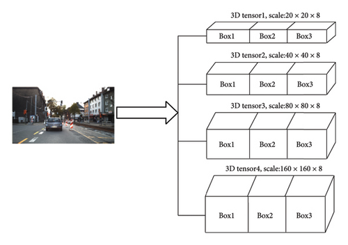
As depicted in Figure 2, the initial step involves dividing the output feature matrix into a series of S × S grids. This division allows for the identification of target centers within individual targets through their corresponding grid units. A grid unit assumes the responsibility for detecting a target if the target’s center resides within its boundaries. Concurrently, each grid unit is equipped to detect up to three bounding boxes. These bounding boxes encompass four coordinate offsets, a confidence score, and a classification for C distinct classes. Hence, the resultant 4D feature matrix, generated from predictions in a single-layer feature matrix, comprises parameters quantified as S × S × [3 × (4 + 1 + C)].
Considering that some areas may have dense targets, the original image grid mapping of a deep-layer feature corresponds to a large area, and the center points of different detection targets may overlap in the same unit cell, which can cause the missed detection of dense targets. Assuming that the input image pixel size is 640 × 640, after 8×, 16×, and 32× down-sampling, the numbers of feature grid cells are 80 × 80, 40 × 40, and 20 × 20, which correspond to large areas in the original image. For dense objects, there may be multiple target centers in the same unit cell. After adding a 4× down-sampling scale, the numbers of feature grid cells are 160 × 160, 80 × 80, 40 × 40, and 20 × 20, which correspond to an increased density and decreased size of the corresponding grid in the original image. The number of small dense targets in the same grid unit is reduced, thereby reducing the probability of missed detection of small objects in dense areas.
3.2. Lightweight Module Improvement
Incorporating shallow feature layers into the model significantly enhances its capacity to detect small targets but concurrently escalates both the parameter count and computational demands. To counterbalance these drawbacks, the strategic implementation of model lightweighting emerges as a crucial intervention. Our empirical investigations, detailed in Section 5.2, underscore the necessity of focusing lightweighting efforts on the network’s neck. The improved lightweight network structure is shown in Figure 3.
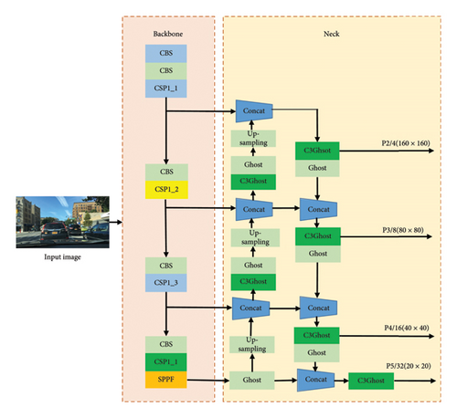
Figure 3 illustrates the substitution of traditional convolution and C3 module with Ghost convolution and C3Ghost module for the neck section. The modified location is indicated in the neck part on the right-hand side. The lightweight module aims to reduce the number of parameters in order to shrink the model size with minimal impact on model accuracy.
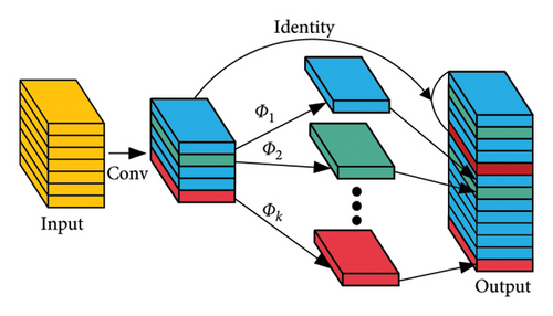
The Ghost is one of the excellent lightweight network modules proposed in 2020, which can effectively reduce the model size. The difference between the Ghost module and traditional convolution is that the Ghost module reduces the number of channels in the convolutional kernel and uses the linear transform (depth convolution) for feature fusion to obtain the same number of channels as traditional convolution. The workflow is as follows: first, feature maps are obtained through traditional convolution, then additional feature maps are generated using linear operations, and finally, the feature matrix obtained by conventional convolution and the multiple feature matrices obtained by linear mapping are concatenated [27]. The Ghost module generates the same number of feature maps with less computation, which can be used to replace standard convolutions in classical convolutional neural networks. The comparison between the conventional convolution and Ghost convolution is shown in Figure 4.
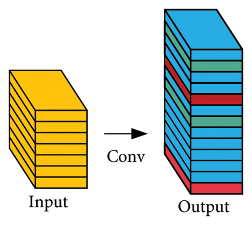
In Equation (4), the numerator represents the computation of traditional convolution parameters, and the denominator represents the computation of the Ghost convolution. n is the number of output channels of traditional convolution, c is the number of input channels, and h′ and w′ denote height and width of the output feature matrix, respectively. k represents the size of the convolution kernel, s is the number of grouped convolutions, and d represents the size of the linear mapping kernel.
The ratio of the computation of the Ghost module to the regular convolution is less than 1. If the number of grouped convolutions s is large, the Ghost module can reduce the computation by approximately s times of standard convolution, achieving similar feature matrices with fewer parameters and computations.
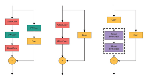
Figure 5 showcases the C3Ghost module. In addition to modifying the base convolution module to the Ghost module in the neck of the network, we also modified the C3 module of the CSP architecture to C3Ghost by changing the bottleneck to the Ghost bottleneck. The C3 module of YOLOv5s has two branches, one with one standard convolution and multiple stacked bottlenecks, and the other with traditional convolution. Finally, the results are concatenated after the two branches have been processed.
3.3. Introduction of Attention Mechanism
The attention mechanism emulates the human visual system’s capacity for selective concentration on pertinent details. This process involves an intentional focus on critical elements while disregarding extraneous information, thereby honing in on the essential data. In the context of road imagery, the background complexity is notably high, especially when it comes to distant entities such as vehicles and pedestrians, which often appear clustered. The challenge intensifies after the application of multiple convolutional layers, making it arduous to differentiate between the feature points of small targets and those of the background. Occasionally, irrelevant background objects might dominate a significant number of feature points, substantially impeding the model’s ability to accurately detect the intended targets. To mitigate the model’s parameter load, we previously incorporated Ghost and C3Ghost modules within the network’s neck. Building on this, we propose the integration of an attention mechanism into the backbone network to further refine detection capabilities.
After conducting a series of experiments, we decided to enhance the C3 module in the backbone network by integrating a global context block (GCNet). This addition aims to amplify the algorithm’s proficiency in feature learning. The specifics of this modification are depicted in Figure 6.

The global context module is an image module that can be used for global context modeling [28]. It is mainly used in detection tasks, particularly for image processing with complex backgrounds, such as natural scenes or city streets. This module has a powerful capability to model long-range dependencies through its nonlocal block, while guaranteeing a lightweight calculation model. The specific structure of the module is illustrated in Figure 7.
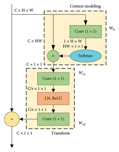
As depicted in Figure 7, the global attention module plays a critical role in extracting comprehensive image features, subsequently integrating these with convolutional features through either element-wise multiplication or addition. This integration significantly augments the model’s comprehensive understanding of the entire image. The process encompasses three main stages: global attention pooling, feature transformation, and feature aggregation. Initially, attention weights are determined via a 1 × 1 convolution and the softmax function, facilitating the extraction of global context features. Subsequently, feature transformation is realized through a 1 × 1 convolution operation. The process culminates in feature aggregation, where the features are amalgamated through summation. Overall, the GC module is proposed as a lightweight method to achieve global context modeling.
As the C3 module has two branches, the improvement of GC module can be attempted in both of them. Various embedding strategies were trialed, revealing that substituting the bottleneck module in the lower branch with a GCBottleNeck substantially elevates computational complexity. Conversely, incorporating the GC module prior to the conventional convolution in the upper branch enhances semantic information with only a marginal parameter increase. Consequently, we consider incorporating the GC module into the upper branch of the C3 module to improve the contextual awareness of the backbone network, as illustrated in Figure 8.

4. Data Preparation
4.1. Datasets
This study utilizes two prominent datasets for the evaluation of road vehicle and pedestrian detection algorithms: the KITTI dataset [29] and the BDD100K dataset [30]. Each dataset is distinct in terms of its composition, target categories, and the scenarios it represents, thereby providing a comprehensive framework for experimental validation.
The BDD100K dataset stands as a substantial and publicly available driving dataset, comprising 80,000 labeled images captured by manually operated vehicles across a spectrum of weather conditions, scenes, and times via key frame sampling. This dataset is characterized by its diverse representations of road conditions, incorporating a wide range of weather scenarios including sunny, cloudy, overcast, rainy, snowy, and foggy conditions, along with various roadway contexts like residential zones, highways, and urban streets. On average, each image features approximately 9.7 cars and 1.2 pedestrians, rendering the BDD100K dataset an exemplary resource for exploring detection tasks across a multitude of scenarios, temporal settings, and road conditions.
The KITTI image dataset is specifically tailored for autonomous driving applications. It consists of 7481 labeled images taken by manually driven vehicles with optical lenses such as grayscale and color cameras. The dataset contains various environments and conditions, including urban areas, rural areas, and highways. The target objects in the KITTI dataset have significant differences in various aspects. For each image, up to 30 people and 15 cars are present, and some targets are small with blurring and occlusion, which adds to the dataset’s challenge.
4.2. Data Analysis
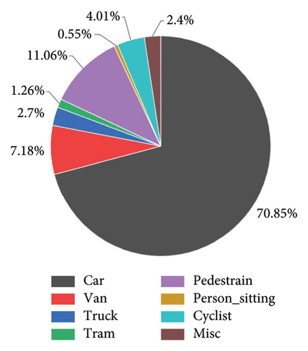
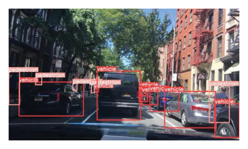
This paper analyzes raw data by selecting the labeled BDD100K and KITTI datasets. Only vehicles and pedestrians are detected in the BDD100K dataset, while vehicles, pedestrians, and bicycles are detected in the KITTI dataset. Therefore, it is necessary to merge some data categories and remove unnecessary ones. The proportional distribution of different target categories in the dataset is shown in Figure 9.

4.3. Data Preprocessing
Given that BDD100K stores annotations such as bounding boxes, categories, and weather conditions in the JSON format, while YOLOv5s training only requires category and bounding box information, it is necessary to design three processes—data filtering, format conversion, and data merging—to construct the final dataset based on the actual situation, as shown in Figure 10.
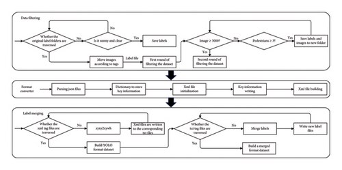
During the data filtering phase, to meet the requirements of small object detection tasks and reduce the consumption of model training, 3000 images with clear targets on sunny days were selected from the 70,000 images in the training set. First, the original label folder was traversed to determine whether each image was annotated as sunny with clear targets. If the requirements were met, the corresponding labels were stored; otherwise, they were ignored. Then, based on the saved labels, the relevant images were moved to obtain the first round of the filtered dataset. Next, the dataset was traversed to check if the number of selected images was greater than or equal to 3000 with at least three pedestrian targets. If these conditions were met, the corresponding labels and images were saved to a new folder, resulting in the second round of the filtered dataset. The distribution of categories in the original and filtered datasets is shown in Figures 11 and 12.
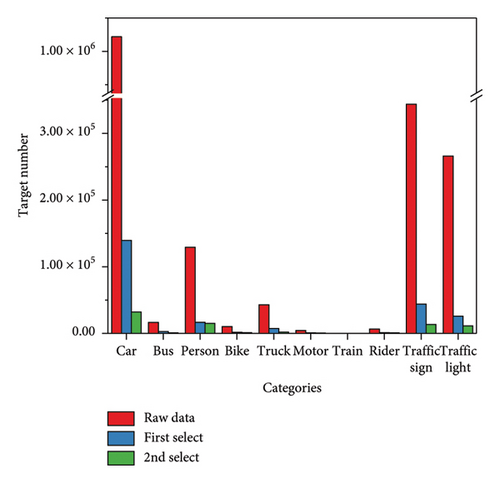
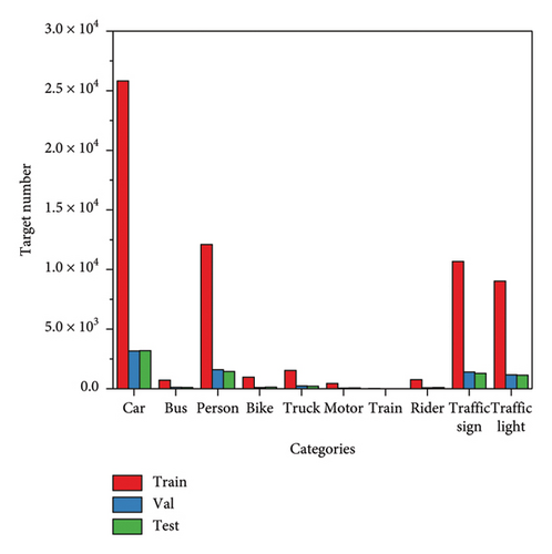
As shown in Figure 11, the proportions of various targets in the original dataset are significantly unbalanced, with vehicles and other categories differing by nearly an order of magnitude. By filtering images with at least three pedestrians, the two rounds of data filtering reduced the overall magnitude difference between the number of vehicles and pedestrians. Figure 12 shows the comparison of the number of targets per category in the filtered training set, validation set, and test set. From the figure, it can be seen that the filtered dataset has a higher proportion of vehicles and pedestrians, and the numbers of these categories are relatively close in the validation and test sets.
During the data consolidation phase, diverse vehicle types such as cars, buses, trucks, and trains within the BDD100K dataset were amalgamated into a unified category designated as “Vehicle”. Concurrently, pedestrians were classified into a distinct category. Subsequent to the amalgamation process, a compilation of 22,737 vehicle instances and 13,531 pedestrian instances was achieved. These instances were systematically allocated to the training, validation, and testing datasets in an 8:1:1 ratio, culminating in a dataset comprising 2400 images for training, alongside 300 images each for validation and testing purposes. Specifically, the training dataset encompasses 28,050 vehicle targets and 12,856 pedestrian targets. Within the validation dataset, composed of 300 images, there are 3504 vehicle targets and 1669 pedestrian targets. Similarly, the testing dataset, also comprising 300 images, contains 2336 vehicle targets and 1340 pedestrian targets. The outcomes of this data merging process are illustrated in Figure 13.
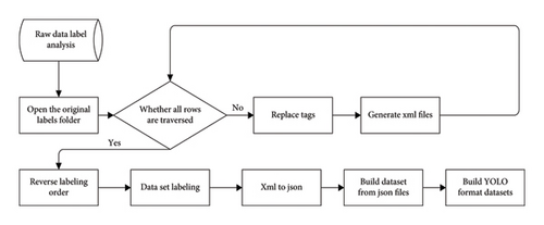
The KITTI dataset was processed through two steps—category merging and format conversion—to construct the final dataset, as shown in Figure 14. First, the original data labels were analyzed by opening the original label folder and traversing all the TXT files within. Each TXT file was then converted into an XML label file in VOC format. After shuffling the labels, the dataset was divided, and the XML files were converted to JSON. Finally, the dataset was constructed in the YOLO format.
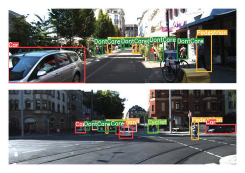
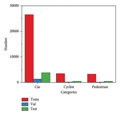
The dataset merges different types of vehicles into one “Car” category, combines pedestrians and sitting persons as one “Pedestrian” category, and treats bicycles as a separate category while ignoring other categories. The merged results are shown in Figure 15. Label category merging is used to alleviate unstable training results caused by large differences in the number of different categories. It enables the effective detection of important road targets under conditions of reduced parameter quantity and provides better verification of different algorithms.

4.4. Analysis of Processed Data
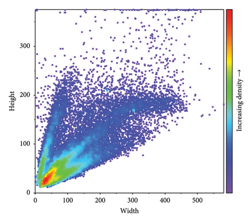
The dataset, following modification, has been designated as “Partial_BDD100K”. An in-depth analysis of this curated dataset was conducted, focusing on the dimensions of the annotated bounding boxes. This examination utilized heat maps to scrutinize the width and height of the targets, alongside the relative proportions of these bounding boxes within the entire image frame. The outcomes of this analysis, particularly the distributions of both the dimensions and their corresponding proportions across the dataset, are encapsulated in the heat maps displayed in Figure 16. This visual representation aids in understanding the spatial characteristics of the targets within the Partial_BDD100K dataset, offering insights into the typical size and space occupancy of the detected objects.
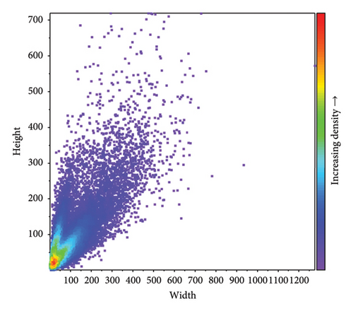
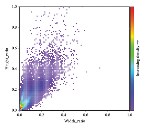
As depicted in Figure 17, the concentration of green and orange-red dots in the lower left corner signifies a higher quantity of targets, while the peripheral areas marked by blue and purple dots indicate fewer targets. A significant portion of the targets within the dataset is approximately 40 × 40 pixels in size. Given this size, it is possible that features of these smaller targets may diminish or even disappear following multiple layers of convolutional pooling. Excessive down-sampling could result in the loss of most target details. In the YOLOv5 network architecture, the maximum down-sampling factor is limited to 32 times, which is a deliberate design choice to mitigate the loss of essential target information to a manageable extent. Given the substantial presence of smaller targets within the Partial_BDD100K dataset, we try to store multiple same-down-sampling feature matrices for different target sizes to retain most of the target information and ensure the extraction of valid information by the backbone network.
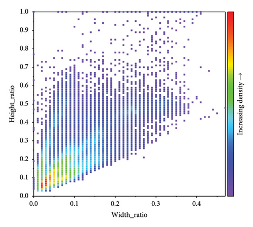
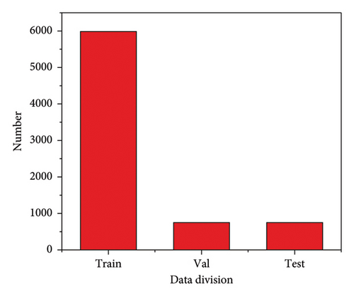
The analysis of the 5985 training images from the consolidated and processed KITTI dataset, as illustrated in Figure 13, reveals a significant concentration of actual targets within the dimension range of 40 × 40 to 100 × 100 pixels (width × height). Furthermore, the aspect ratio (width to height) of these targets predominantly falls within the range of 0.05 × 0.1 to 0.1 × 0.2. In addition, the number of images in the training, validation, and test sets is shown in Figure 17, and the number of targets per category is shown in Figure 18. The statistical insight underscores a notable clustering of small target sizes within a specific dimensional spectrum, highlighting the importance of tailoring detection algorithms to effectively recognize and process targets within these small size and aspect ratio ranges.
4.5. Statistics of Road Target Size
Given the average dimensions of the KITTI dataset and the Partial_BDD100K dataset at 1280 × 720 and 1242 × 375 pixels, respectively, it’s evident that the image resolutions substantially exceed those typically found in the COCO dataset. Hence, establishing the threshold for small targets in road traffic datasets at 32 × 32 pixels is a logical approach. Road traffic image datasets feature a diverse array of object sizes, allowing for categorization into small, medium, and large targets based on their scale. Meanwhile, a statistical analysis is carried out on the number and proportion of small targets in the training set category labels [31].
The number of label boxes for each scale is listed in Table 2. It can be observed from the table that the number of small objects in the KITTI training set is 5429, accounting for 14.64% of the total, in the Partial_BDD100K dataset, the number of small objects is 18,397, accounting for 31.02%, indicating that the quantity of small objects in road scene datasets is relatively high, but the overall area sizes are only 1.02% and 2.50%, respectively. The prevalence of small objects underscores the challenges faced in the road scene, where large and medium-sized objects dominate the annotations, but small objects, because of their limited pixel, undergo significant feature attenuation post-down-sampling, hard to detect. This observation emphasizes the importance of devising detection algorithms that are particularly sensitive to the nuanced features of small objects, ensuring comprehensive and accurate scene analysis in varied road environments.
| Dataset | Target scale | Number | Percentage of target boxes (%) | Percentage of total area (%) |
|---|---|---|---|---|
| KITTI | Small target (0 < area < 32 × 32) | 5429 | 14.64 | 1.02 |
| Medium target (32 × 32 < area < 96 × 96) | 17,149 | 46.24 | 17.08 | |
| Big target (96 × 96 < area < +∞) | 14,507 | 39.12 | 81.90 | |
| Partial_BDD100K | Small target (0 < area < 32 × 32) | 18,397 | 31.02 | 2.50 |
| Medium target (32 × 32 < area < 96 × 96) | 16,191 | 27.30 | 15.22 | |
| Big target (96 × 96 < area < +∞) | 24,715 | 41.68 | 82.28 | |
5. Experiment and Results Analysis
In this section, experiments were conducted on the KITTI and Partial_BDD100K datasets to evaluate the proposed algorithm. We detailed the experimental framework, parameter configurations, and results. Furthermore, we compared the experimental outcomes with those of conventional object detection algorithms. Through these experiments, the enhanced YOLOv5 algorithm was validated, demonstrating its superior detection performance.
5.1. Experimental Environment Framework and Setup
The application of deep learning in multiple fields is becoming increasingly common. Therefore, open-source frameworks are widely used to adapt to different environments. In this study, experiments were conducted using the Pytorch framework based on the Python language. The hardware environment consisted of an AMD Ryzen 9 5900HX with Radeon Graphics CPU and an NVIDIA GeForce GTX 3080 GPU, and the integrated development environment used was Pycharm2020.3.
The initial learning rate of the experiment was set to 0.0032 using a dynamic descent method, with a learning decay factor of 0.1. Because of hardware and memory limitations, a batch size of 16 was used, and the training iteration was set to 300. The input image size was uniformly set to 640 × 640.
For the training configuration, the pretraining weight file of YOLOv5s is selected. For hyper-parameter settings, the initial values of optimizer-related parameters such as learning rate, learning rate momentum, and weight decay coefficient are consistent with the baseline model, and the same is true for parameters related to preheat learning, loss function, and data enhancement.
In the training phase, following the training strategy of YOLOv5s algorithm, including the data enhancement strategy, the size and aspect ratio of the backbone network, and the predefined anchors, the same training strategy is adopted for different models in order to achieve fair competition among different models to a certain extent.
5.2. Detection Results on Partial_BDD100K Dataset
Experimental evaluations were conducted on the Partial_BDD100K dataset. Initially, the optimal position for the Ghost module was determined by comparing the performance of various improvement locations. Subsequently, the detection results of the C3CBAM and C3GC modules were compared to determine the optimal attention mechanism enhancement scheme. Ultimately, a comparison with classical models was performed to verify the feasibility of the proposed improvement scheme.
5.2.1. Lightweight Module Comparison Experiment
This paper attempts to integrate lightweight modules into different parts of the network to further reduce the model’s parameter count while ensuring that detection accuracy does not significantly decrease. As this experiment is only conducted to compare the effectiveness of different modules, and the model training has reached a converged state after 150 iterations, 150 iterations were performed under different conditions to evaluate the detection performance of models integrated at different positions, providing a reference basis for subsequent experiments. Comparative experimental results are shown in Table 3.
| Algorithm | Vehicle AAP (%) | Pedestrian AAP (%) | mAP @0.5 (%) | Params | MB | FPS |
|---|---|---|---|---|---|---|
| YOLOv5s_Ghost_backbone | 69.2 | 45.3 | 57.2 | 5,081,671 | 10.0 | 80.0 |
| YOLOv5s_Ghost_all | 65.3 | 46.6 | 56 | 3,678,423 | 7.4 | 74.6 |
| YOLOv5s_Ghost_neck | 71.8 | 51.4 | 61.6 | 5,612,271 | 11.0 | 82.6 |
Table 3 demonstrates that substituting the standard convolution and C3 convolution in the network’s neck with Ghost and C3Ghost modules yielded the highest accuracy on the test set and facilitated quicker detection speeds compared to the incorporation of Ghost modules in other locations. Consequently, in subsequent experiments, standard convolutions and C3 modules are replaced in the neck to leverage these advantages.
5.2.2. Attention Mechanism Comparison Experiment
As significant improvements have already been made to the network’s neck, different attention mechanisms will be introduced to the backbone of the network to further enhance detection performance. Comparative experiments will be conducted on the Partial_BDD100K dataset, and 150 iterations will be performed under various conditions to verify the effects of embedding different attention mechanisms into the backbone.
Table 4 shows that replacing the C3 modules in the backbone network did not significantly improve performance on the Patial_BDD100K dataset. Therefore, further experiments on the KITTI dataset are needed to determine the optimal module.
| Algorithm | Vehicle AAP (%) | Pedestrian AAP (%) | mAP @0.5 (%) | Params | MB | FPS |
|---|---|---|---|---|---|---|
| YOLOv5s C3CBAM_backbone | 73.3 | 52.3 | 62.8 | 7,062,955 | 13.8 | 66.7 |
| YOLOv5s C3GC_backbone | 72.5 | 53.3 | 62.9 | 7,371,523 | 14.4 | 63.3 |
5.2.3. Classical Model Comparison Experiment
On the Partial_BDD100K dataset, vehicle and pedestrian detection were conducted. By comparing with classic models, such as SSD and YOLOv5s, it was found that the proposed model improved the category average precision by 28.2% relative to SSD and 3.3% relative to the baseline YOLOv5s model at a 0.5 confidence level. In summary, the model improves the overall detection accuracy while bearing a reduced cost of lower detection speed.
From Table 5, because of the presence of many interference objects and small targets in the BDD100K dataset, and only 3000 selected images were used for experimental research, the overall detection performance was suboptimal. However, the improvement in overall detection accuracy relative to the baseline model was relatively large, indicating that the improved model has certain research value in comparative experiments.
| Algorithm | Vehicle AAP (%) | Pedestrian AAP (%) | [email protected] (%) | FPS |
|---|---|---|---|---|
| SSD [32] | 54.9 | 31.5 | 43.2 | 32.6 |
| YOLOv3s | 69.0 | 50.6 | 59.8 | 91.2 |
| YOLOv5s | 73.4 | 53.4 | 63.4 | 82.6 |
| YOLOv5s-LGC | 76.7 | 56.7 | 66.7 | 63.2 |
- Note: Bold values indicate the maximum values and also the best results.
5.3. Detection Results on the KITTI Dataset
Given the modest differentiation in the verification performance of various attention mechanisms on the Partial_BDD100K dataset, further comparative experiments were conducted on the more extensive KITTI dataset. Subsequent comparisons of different models were undertaken to substantiate the viability of the proposed enhancements.
5.3.1. Attention Mechanism Comparison Experiment
The same 150 iterations converge, and the final test results for 150 iterations are presented in Table 6.
| Algorithm | Car AAP (%) | Cyclist AAP (%) | Pedestrian AAP (%) | mAP @0.5 (%) | MB |
|---|---|---|---|---|---|
| YOLOv5s_C3CBAM_backbone | 97.9 | 92.3 | 86.3 | 92.2 | 14.4 |
| YOLOv5s_C3GC_backbone | 98.0 | 93.3 | 86.5 | 92.6 | 15.1 |
From Table 6, it is evident that the C3GC improvement approach has boosted the detection accuracy of the test set by 0.4% compared to the C3CBAM enhancement method. To attain a noteworthy improvement in the mAP metric without significantly increasing the number of parameters, the C3GC module was chosen to replace the C3 module in the backbone.
5.3.2. Classical Model Comparison Experiment
The proposed YOLOv5s-LGC model was compared with classic models including Faster R-CNN, SSD, and improved YOLOv3s, with YOLOv3s and YOLOv7s being networks of the same depth and width as YOLOv5s. The comparative results are presented in Table 7.
| Algorithm | Car AAP (%) | Pedestrian AAP (%) | Cyclist AAP (%) | mAP @0.5 (%) | FPS |
|---|---|---|---|---|---|
| Literature [33] | 86.7 | 87.4 | 84.4 | 86.2 | 37.6 |
| Literature [34] | 88.5 | 51.0 | 66.0 | 68.5 | 45 |
| Faster R-CNN [35] | 74.1 | 83.3 | 74.1 | 77.6 | 13.2 |
| SSD [32] | 85.3 | 51.0 | 57.6 | 63.4 | 56.0 |
| YOLOv3s | 97.7 | 86.3 | 94.0 | 92.7 | 90.1 |
| YOLOv5s | 98.0 | 87.0 | 93.5 | 92.8 | 75.2 |
| YOLOv7s | 97.3 | 81.2 | 92.1 | 90.2 | 79.4 |
| YOLOv5s-LGC | 97.9 | 90.0 | 95.3 | 94.4 | 60.6 |
- Note: Bold values indicate the maximum values and also the best results.
On the KITTI test set, the proposed YOLOv5s-LGC algorithm has achieved a certain improvement in detection accuracy compared to references 29 and 30, as well as classic detection algorithms, demonstrating the effectiveness of adding shallow feature layers, adding Ghost modules, and increasing GC attention mechanisms. Within the scope of this research, the YOLOv5s-LGC algorithm showed an increase in accuracy, though accompanied by a marginal reduction in FPS.
Given the study’s focus on detecting small objects in autonomous driving contexts, priority is placed on improving algorithmic accuracy while maintaining suitable detection speeds. For applications such as low-speed driving or parking assistance, a performance threshold of 30 FPS is considered adequate. Meanwhile, for high-speed driving or more complex autonomous navigation scenarios, a benchmark of 60 FPS is deemed satisfactory. Therefore, the proposed algorithm effectively meets the criteria for real-time performance.
5.4. Visualization Test Results on the KITTI Dataset
The mAP curves of YOLOv3s, YOLOv5s, and YOLOv5s_LGC during 300 iterations of experiments on the KITTI validation set are depicted in Figure 19.
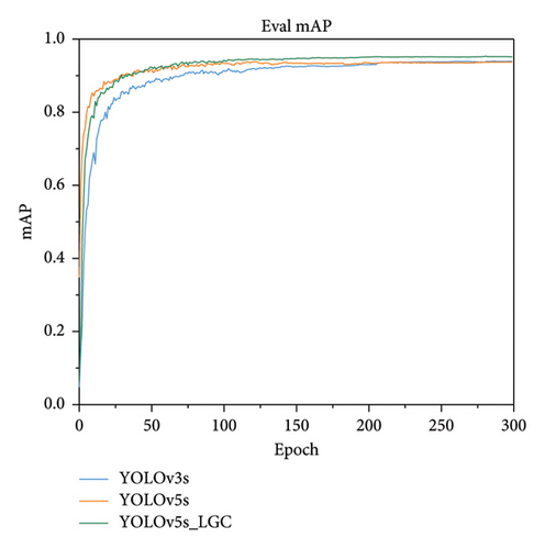
From Figure 19, the mAP values gradually converge at 150 iterations, and the proposed YOLOv5s-LGC model has partially improved in terms of convergence speed and accuracy during the iterations, which indicates that the model detects better.
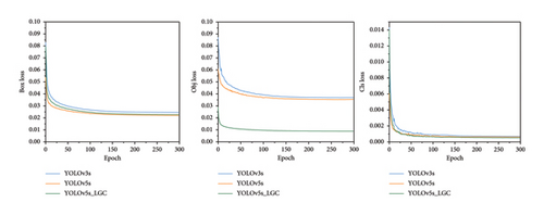
Figure 20 illustrates the curves for bounding box loss, confidence loss, and class loss over 300 iterations. As the model iterates, the losses gradually converge, particularly after 200 iterations. The proposed YOLOv5s-LGC model achieves a faster convergence rate compared to the original YOLOv5s and YOLOv3s models, exhibiting lower confidence and class losses. This underscores the improved model’s effectiveness on the KITTI dataset.
To visually demonstrate the detection performance of the proposed model on traffic targets, images numbered 000073 and 000770 from the test set were selected for qualitative evaluation, presenting the target detection results of YOLOv3s, YOLOv5s, and the proposed YOLOv5s-LGC algorithm, respectively. This is shown in Figure 21.
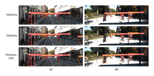
As observed in Figure 21, on the image with label 000073, the YOLOv3 algorithm detected six pedestrians and two bicycles, YOLOv5s detected six pedestrians and three bicycles which additionally included the bicycle in the lower-right corner of the image, while the proposed YOLOv5s-LGC algorithm detected seven pedestrians and three bicycles, which included an additional pedestrian in the middle of the image. On the image with label 000770, the YOLOv3s algorithm incorrectly identified a bicycle on the left as a pedestrian, YOLOv5s algorithm failed to detect the target at all, while the proposed YOLOv5s-LGC algorithm was able to successfully detect the bicycle target and show slight improvement in detection precision for different categories. This effect can also be seen from the obtained scores of detection categories, indicating that the improved algorithm has a certain promotion effect on image target detection.
To visually display the advantages of the small target detection of the method in this paper, two images of small target objects that are far away from the camera are selected on the KITTI dataset, respectively, as shown in Figure 22.
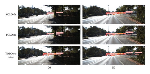
From image 001286, it can be observed that YOLOv5s-LGC detected some pedestrian targets that were not detected by the other two models. The results of detection from image number 001466 show that YOLOv5s has mainly improved in accuracy. According to the program statistics, the improved YOLOv5s-LGC detected four pedestrians, four cars, and one bicycle, which is significantly more than the other models in terms of quantity. Thus, the YOLOv5s-LGC algorithm has improved the detection of small targets on the road to a certain extent.
To sum up, the original YOLOv5s model has a slightly poorer performance in detecting small targets in the distance, with lower accuracy and some missing target detection. However, the YOLOv5s-LGC algorithm proposed in this paper has improved the detection ability of small targets in the image and further improved the category score. This indicates that by fusing shallow features, improving the backbone network, and introducing attention mechanisms, strong semantic information is obtained from the pictures with detailed information, thus improving the detection ability of the network model and reducing the missed detection rate.
5.5. Ablation Experiments
This paper proposes three main improvements to the YOLOv5s algorithm: L: introducing shallow feature layers to tackle the issue of small target detection; G: replacing conventional convolutions and C3 modules with Ghost convolutions and C3Ghost modules, respectively; C: introducing GC attention mechanism to address background interference. To validate the necessity of different modules for the final results, ablation experiments were conducted on the KITTI dataset. Table 8 displays the model parameter and detection results in order of increasing levels of improvement: shallow features, Ghost improvements, and attention mechanism improvements.
| Algorithm | L (add shallow) | G (ghost) | C (GC module) | Validation set mAP @0.5 (%) | Test set mAP @0.5 (%) | Params | MB | FPS |
|---|---|---|---|---|---|---|---|---|
| YOLOv5s | 93.7 | 92.8 | 7,018,216 | 13.7 | 71.9 | |||
| YOLOv5s-L | √ | 94.7 | 94.3 | 7,719,296 | 15.2 | 66.7 | ||
| YOLOv5s-G | √ | 93.5 | 92.7 | 5,612,271 | 11.2 | 72.1 | ||
| YOLOv5s-C | √ | 94.5 | 94.1 | 7,615,324 | 15.1 | 67.8 | ||
| YOLOv5s-LG | √ | √ | 94.2 | 93.6 | 6,023,296 | 12.0 | 65.8 | |
| YOLOv5s-LGC | √ | √ | √ | 95.2 | 94.4 | 6,338,212 | 12.6 | 60.6 |
- Note: Bold values indicate the best values of the effect, i.e., the larger the better in the mAP and FPS metrics, and the smaller the better in the Params and MB metrics.
Firstly, we added each of the three methods L/G/C to the baseline model to analyze their independent contributions. It can be seen from the table that the parameters of the YOLOv5s-L model increased by about 7.0 × 10⁵ compared to the benchmark YOLOv5s, and the model size increased by 1.5M. Under the IoU threshold of 0.5, the mAP of the validation and testing sets increased by 1.0% and 1.5%, respectively, and the overall detection accuracy improved. The detection speed was 66.7 FPS, and the detection time for a single image was 15.0 ms with the addition of shallow feature fusion, which increased by 1.1 ms compared to the original YOLOv5s detection time. The experimental results of the improved YOLOv5s-L model show that adding shallow features fusion is conducive to improve the accuracy of detection targets, and it may achieve a certain degree of improvement for some difficult-to-detect targets, but the model capacity and parameter quantity increase. For the YOLOv5s-G model, the amount of parameters in the model is reduced by about 1.4 × 10⁶, the model size is reduced by 2.5M, and the detection speed is the highest at 72.1 FPS. Yet, its accuracy is only reduced by 0.1% on the test set, which shows its excellent performance in balancing accuracy and speed. For the YOLOv5s-C model, its detection accuracy improves by 0.8% on the validation set and 0.3% on the test set, proving that the addition of this module also has a positive effect on model detection.
Secondly, for the improved YOLOv5s-LG model, the number of parameters decreased by about 1.7 × 10⁶ compared to the YOLOv5s-L model, and the model size decreased by 3.2M, which is 1.7M less than the benchmark YOLOv5s model. Under the 0.5 threshold, the mAP of the validation and testing sets decreased by 0.5% and 0.7%, respectively, compared to the YOLOv5s-L model, and increased by 0.5% and 0.8%, respectively, compared to the original YOLOv5s model. The detection speed did not change significantly. The experimental results of the YOLOv5s-LG model show that replacing the conventional convolution in the neck of the network with a lightweight Ghost convolution significantly reduces the model’s parameter quantity, which reduces the deployment difficulty of the model, although the accuracy has decreased to some extent.
Finally, for the YOLOv5s-LGC model, the model parameters increased by only 3.1 × 10⁵ and the model size increased by only 0.6M. Under the 0.5 confidence, the average precision of all categories on the validation set reached 95.2% and reached 94.4% on the testing set, an improvement of 1.6% over the benchmark YOLOv5s model. In summary, the predictive results of the improved YOLOv5s-LGC algorithm are optimal, which not only improves the overall prediction accuracy but also reduces the model’s parameter quantity.
In theory, changing the conventional convolution to the Ghost module will increase the detection speed of the model; however, experiments show that the detection speed does not show significant improvement on both datasets used. For the problem that the detection speed decreases while the model size decreases after adding the Ghost module to the model neck, it is analyzed that there are roughly the following reasons: (1) Memory bandwidth limitation. The addition of the Ghost module may lead to memory bandwidth limitation, which affects the inference speed of the model. Since the Ghost module requires channel interaction operations, this may result in more memory accesses, which increases the burden on memory bandwidth. (2) Increased data dependency. The model may need more time to wait for the computation results of the previous layer, thus reducing the overall inference speed.
5.6. Generalizability Experiments
Since the Ghost convolution layer was experimentally determined to work the best, to validate the generalization of the model, we decided to add the UA-DETRAC dataset to validate the model performance. To contrast with the previous paper, we use SSD, YOLOv3s, YOLOv5s, and YOLOv7s algorithms for comparison, as shown in Table 9.
| Algorithm | Car AAP (%) | Bus AAP (%) | Van AAP (%) | mAP @0.5 (%) |
|---|---|---|---|---|
| SSD [32] | 79.3 | 77.2 | 70.1 | 76.2 |
| YOLOv3s | 96.2 | 84.8 | 92.1 | 92.3 |
| YOLOv5s | 93.2 | 88.3 | 95.2 | 92.7 |
| YOLOv7s | 96.3 | 83.4 | 91.8 | 90.8 |
| YOLOv5s-LGC | 96.8 | 91.2 | 94.5 | 94.9 |
- Note: Bold values indicate the best values of the effect, i.e., the larger the better in the mAP metric.
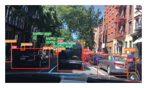
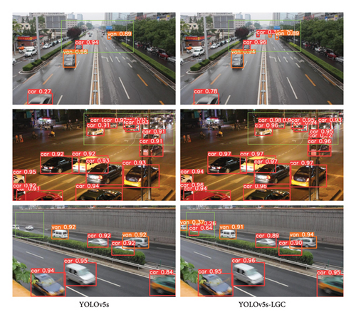
As can be seen from Table 9, in the UA-DETRAC dataset, our method is still advanced with higher accuracy compared to other mainstream methods. Figure 23 shows the experimental comparison between YOLOv5s and our method, where the green boxes indicate that our method detects more small targets.
6. Conclusion
- •
Firstly, we pointed out some difficulties in detecting small objects and analyzed and preprocessed the KITTI and Partial_BDD100K datasets.
- •
Secondly, the YOLOv5s model with good performance on a general dataset was selected as the baseline model. Based on YOLOv5s, we attempted to incorporate shallow features, Ghost modules in the neck, and GC attention mechanism in the backbone to obtain deep features.
- •
Finally, the optimized network model was used for road object detection, and comparative experiments were established to verify the robustness of the model. The results showed that on the KITTI and Partial_BDD100K datasets, YOLOv5s-LGC can improve the mAP at 0.5 confidence to 94.4% and 66.7%, respectively, which is higher than other methods, and with fewer parameters than the YOLOv5s model, demonstrating the effectiveness and robustness of this approach.
- •
The detection effectiveness in some scenarios needs to be improved. In actual road traffic scenarios, there are often various special situations, such as occasional traffic accidents and natural environments, which will have a certain impact on the object detection. This study mainly focused on the research on small object detection and provided less training on models for different situations. Further research can be conducted for different scenarios in the future.
- •
The dataset needs to be further enriched. The datasets used in this article are mostly public data for autonomous driving scenarios, and because of the limited experimental conditions, only part of the data was used for the experiment to verify the performance of different modules. In the future, the dataset can be expanded on the basis of some original datasets to improve the richness of the dataset.
- •
There is still room for improvement in some modification schemes. After a lot of experimentation and attempts, the methods of adding shallow feature layers, lightweight module improvement, and introducing attention mechanisms were finally determined to improve the YOLOv5s model. However, with the rapid development of technology in the world today, in the field of object detection, further improvement plans can be sought for anchor-free series, transformer series, YOLOv7 series models, etc.
Conflicts of Interest
The authors declare no conflicts of interest.
Author Contributions
Sheng Tian: conceptualization, supervision, funding acquisition, and formal analysis. Kailong Zhao: data curation, methodology, software, validation, writing – original draft, and reviewing and editing. Lin Song: writing – original, visualization, and validation.
Funding
This work was supported in part by the Natural Science Foundation of Guangdong Province under Grant: 2021A1515011587.
Acknowledgments
This work was supported in part by the Natural Science Foundation of Guangdong Province under Grant: 2021A1515011587.
Open Research
Data Availability Statement
The datasets generated during and/or analyzed during the current study are available from the corresponding author on reasonable request.


