A Model for Predicting Short-Term Operating Speeds of Compact Passenger Vehicles on Interchange Ramps Within Urban Expressway Networks
Abstract
The prediction of operating speed plays a crucial role in road design and safety assessment, especially on complex urban expressway interchange ramps. This task is challenging due to various influences like road conditions, traffic dynamics, and driver behavior. This study aims to identify the optimal model configuration for predicting operating speeds on urban expressway interchange ramps. Three models are established: a short-term operating speed model based on a generalized linear model (GLM), a GLM incorporating for spatial correlation (GLMS), and a deep neural network model considering spatial correlation (DNNS). Each model incorporates considerations for the impact of the plan, profile, and other facets of the interchange ramp in urban expressways. Naturalistic driving experiments are conducted in Shanghai, 70% for model calibration and 30% for validation. Comparative analysis shows that the DNNS model outperforms the others, effectively capturing speed fluctuations along the interchange ramp, demonstrating its robustness and generalization capabilities.
1. Introduction
Operating speed is defined as the safe speed that an average skilled driver can maintain under prevailing road conditions, traffic density, favorable weather conditions, and other relevant factors. Predicting the operating speed of vehicles assumes a pivotal role in the evaluation of road safety and the implementation of safe operational controls [1]. However, urban expressway interchange ramps boast intricate geometric configurations, rendering it challenging to precisely anticipate the operating speed on these ramps [2, 3]. Interchange ramps often become sites of traffic accidents stemming from incongruous speed connections between the ramp subsystems of interchanges or among different subsystems [4]. Consequently, interchange ramps are commonly acknowledged as high-risk segments that exert a substantial impact on the overall safety of the road system [5, 6].
Establishing a precise model for predicting operating speeds at urban expressway interchange ramps is of paramount importance, ensuring the safety and effective control of vehicle operations on these ramps, and providing a theoretical foundation for safety evaluations [7]. Noteworthy progress has been made by some researchers in predicting operating speeds on ramps [8–10]. Rímalová et al. [11], based on floating car data, employed a functional regression model to evaluate the impact of curvature and auxiliary lanes on driving speed and predicted driving speed on an expressway interchange in Brno, Czech Republic. Brewer et al. [12] utilized data from the Natural Driving Study (NDS) conducted as part of the US Highway Strategic Research Program Phase 2 (SHRP2) to establish the relationship between the design speed of highway ramps and the speed chosen by drivers on these ramps. Liapis et al. [13] employed regression models to analyze operating speed at curved ramp sections of minor interchanges. These studies provide valuable insights into predicting operating speed and enrich our understanding of driving behaviors [14]. However, existing research predominantly centers on the operating speed of mountainous highways or expressways, with comparatively limited exploration into the operating speed of urban expressway interchange ramps. Moreover, research on operating speed lies in establishing relationships between operating speed and road geometric characteristics at specific sections and cannot accurately anticipate speed fluctuations across the entire ramp.
This study conducts natural driving experiments to formulate three predictive models for operating speeds of compact passenger vehicles on urban expressway interchange ramps. These models encompass a generalized linear model (GLM), a GLM incorporating spatial correlation (GLMS), and a deep neural network model considering spatial correlation analysis (DNNS). Subsequently, the proposed models are applied to predict the speed of other interchange ramps and are compared to assess their generalization ability and prediction accuracy. The DNNS model can generate a continuous speed curve for vehicles traveling on the ramp, which can serve as a valuable tool for understanding the speed distribution of vehicles on ramps. This understanding assists in optimizing ramp geometric design, conducting road safety assessments, identifying hazardous areas, and providing guidance for road design or traffic management.
2. Literature Review
2.1. Analysis of Factors Influencing the Operating Speed of Ramps
Recognizing that the operating speed of vehicles is primarily influenced by road alignment conditions, most researchers utilize road geometry to forecast the operating speed, such as slope, curvature, and other factors [15, 16]. Jafarov et al. [17] conducted an analysis of the operating speeds of vehicles on 18 ramps within 10 highway interchanges in Moscow. They formulated a model for operating speed and acceleration, utilizing the ramp slope as the sole input variable. They employed a linear regression methodology to predict operating speed. In a separate investigation, Xie et al. [18] scrutinized the driving performance of vehicles on mountain grade separation ramps and introduced a speed prediction method that takes into account curvature, curve length, and cumulative steering angle. Gong et al. [19] identified that curve factors, specifically curve radius and length, predominantly influence the driver’s speed choice. Hashim et al. [20] established a speed profile model for two-lane rural roads by considering the geometric design of horizontal and vertical alignments. Paolo et al. [21] developed an operating speed model for low-capacity roads, incorporating factors such as relative sight distance, radius, and curvature change rate. Hence, based on the literature discussed earlier, this study develops models to predict vehicle operating speeds on interchange ramps. It considers factors such as slope gradient, curvature, and the length of vehicle entrance to a ramp.
Additionally, the velocity of vehicles on ramps is influenced by spatial correlation. Spatial correlation describes the behavior of a vehicle’s speed at a specific point during its journey. This speed is influenced not only by the immediate geometric characteristics of the road at that point—such as curvature, slope, and surface conditions—but also by the state of the trajectory at preceding locations (i.e., adjacent points along the vehicle’s trajectory) and the cumulative effect of the vehicle’s speed at these locations. This correlation highlights the continuity and dynamism of driving behavior, indicating that the vehicle’s motion is a continuous process that evolves over time and space. Consequently, the current speed state is a cumulative response to past road conditions and speed states. While the immediate geometric characteristics of the road have been considered in previous studies, spatial correlation has often been overlooked. Recognizing spatial correlation is pivotal because, for interchange ramps, speed fluctuations frequently manifest in closely observed spaces, where the operating speed of a vehicle at a particular trajectory point heavily relies on the operating speed of the preceding trajectory point and alterations in road geometric conditions [22, 23]. Therefore, in our study, the GLMS and the DNNS introduce intermediate speed parameters (representing vehicle speeds at preceding trajectory points), intermediate curvature parameters (indicating road curvature at preceding points), and intermediate slope parameters (reflecting road slope at preceding points) to consider the spatial correlation of vehicle travel speed and enhance the accuracy of predicting vehicle speeds on ramps.
2.2. Operating Speed Prediction Methods
Recently, various models have been employed for speed prediction, encompassing linear regression [24], GLM, random effect models [25, 26], and neural network models [27]. Among these models, the multiple linear regression model stands out as the most commonly employed. For instance, Yao et al. [28] utilized the linear regression method to formulate a speed prediction model for super long tunnels on highways, considering tunnel geometric parameters. Banihashemi et al. [29] applied the linear regression method to establish a speed model for rural two-lane highways. Thiessen et al. [30] used a GLM to predict speeds at the midpoint of straight segment roads, leveraging panel data from straight segments in Canada. Maji et al. [31] crafted three operating speed prediction models through stepwise multiple linear regression analysis.
The random effects model primarily explains the random variations among individuals. However, it necessitates a well-structured dataset and adequate data to achieve reliable estimation results. Bassani et al. [32] established a random effects model using environmental parameters related to road geometry and lighting conditions to predict the average speed of vehicles. Their model assumes that the operating speeds at different points during vehicle travel are independent of each other. However, both the GLM and the random effects model merely account for the impact of road geometry on vehicle speed, failing to consider the influence of spatial correlation on travel speed.
Neural network models excel in managing intricate nonlinear relationships, showcasing robust learning and predictive capabilities, and autonomously discerning patterns within data [33]. Wu et al. [34] formulated a short-term prediction model for lane driving speed within extra-long tunnels, employing the temporal Transformer framework. The constructed speed prediction model achieves a commendable accuracy of 97.82%. In a previous study, Wu et al. [35] devised a speed prediction model based on a gray neural network, amalgamating the advantages of the low data requirements inherent in the gray prediction model and adaptive capabilities of neural networks. However, despite the effectiveness of these models in capturing the temporal dependencies of speed sequences in time-series prediction, they fail to simultaneously account for road alignment conditions and spatial correlations—factors that are crucial for accurately forecasting travel speed.
To investigate the impact of road alignment conditions and spatial correlation on driving speed in urban interchange ramps, this study employs the GLM as a baseline. It integrates the Exponential Moving Average (EMA) method to account for spatial correlation in vehicle operations. Building on this, the study enhances the GLM and neural network models to incorporate spatial effects on vehicle speed, enabling accurate predictions of speed fluctuations across the entire ramp.
3. Data Acquisition
3.1. Natural Driving Experiment
We conducted natural driving experiments in Shanghai (SNDD) and selected time periods during which vehicles were relatively less influenced by surrounding traffic conditions for data collection. The experimental vehicles adopt the small car design specified in the Chinese standard “Technical Standards for Highway Engineering” (JTG B01-2014), with a wheelbase of ≤ 7 m and a specific power of > 15 kW/ton. These vehicles are outfitted with onboard Data Acquisition System (DAS) which comprise devices such as Doppler radar, triaxial accelerometers, and Global Positioning Systems (GPS), event button, four synchronized high-definition cameras, and data integration recorder all operating at a sampling frequency of 10 Hz.
Drivers navigate their vehicles continuously to collect data in real conditions according to their customary driving behavior and patterns. The DAS integrated within the test vehicle, diligently captures and records driver behavior metrics, commencing approximately 90 s after the ignition of the vehicle’s engine and persisting until its subsequent shutdown. Consequently, every datum recorded by the computerized system, inclusive of video footage and GPS data, can be construed as a comprehensive portrayal of a driver’s travel behavior.
From the data obtained from these experiments, we have selected trajectory data segments of vehicles navigating within urban expressway interchange ramps for our research [36]. Specific trajectory data tailored to its research objectives and subjects are employed, encompassing the following: (1) GPS data capturing vehicle speed within the mainline area of urban expressway interchange ramps. This data concentrates on sections unaffected by merging and diverging zones. (2) Video data of vehicles driving within the urban expressway interchange ramp area. The videos feature forward-facing views, facilitating the evaluation of road traffic conditions during vehicle movement.
3.2. Interchange Ramp Data Extraction
The DAS in our experiments captures all the characteristic parameters of the experimental vehicles from startup to shut down and consolidates them into a unified CSV file. The data file aligns with a consistent timeline shared with the corresponding video data. The current dataset comprises 9207 CSV files along with their corresponding video records. To acquire trajectory data of vehicles on ramps, data cleaning and extraction of urban expressway interchange ramp trajectory data are undertaken as following: (1) Given the study’s emphasis on travel records on urban expressways, where the process of entering and exiting these expressways typically involves longer driving times, CSV files smaller than 1000 KB are excluded, resulting in 3556 remaining records. (2) The latitude and longitude data in the CSV files are imported into ArcMap software to identify concentrated travel trajectories around urban expressway interchanges. (3) Given the significant speed differences between the ramp merging/diverging areas and the mainline sections, this study focuses on the region between the noses of the ramp diverging triangle and the merging triangle, excluding the acceleration and deceleration lanes. Trajectory data from this area are extracted using the K-Nearest Neighbors (KNN) algorithm, with the number of neighbors set to 1 to identify the nearest point to the noses of both the diverging and merging areas. Based on these points, the trajectory data between them are retrieved from the CSV file. Finally, the accuracy and validity of the extracted trajectory data are evaluated by comparing it with actual observed video and trajectory data. The final dataset comprises a total of 974 interchange ramp trajectory data. The extracted interchange ramps encompass three types: ① direct ramps, ② loop ramps, and ③ indirect ramps, as shown in Figure 1. There are 600, 115, and 259 trajectory data for the three types of interchange ramps.
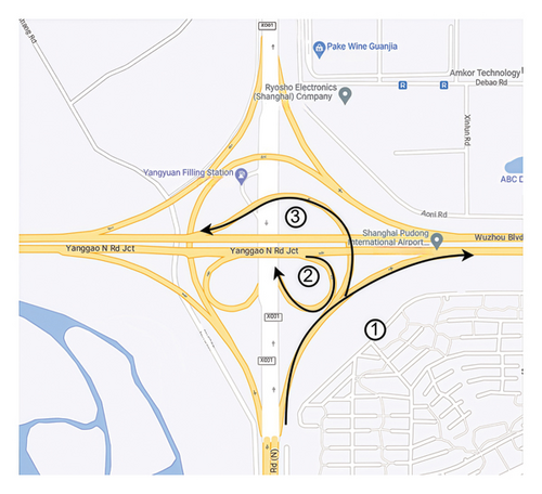
These data serve as the foundation for subsequent analysis and prediction. Geometric parameters and types of interchange ramps are delineated in Table 1. Furthermore, the extracted interchange ramps in this study are all single-lane ramps. The road widening caused by the horizontal curve is not significant due to its location on the ramp. Moreover, the lighting conditions remain consistent along the entire road for each interchange ramp.
| No. | Slope (%) | Radius of the longest horizontal curve (m) | Length of interchange (m) | No. | Slope (%) | Plan curvature radius (m) | Length of interchange (m) |
|---|---|---|---|---|---|---|---|
| Direct interchange ramp | |||||||
| 1 | −5.78 | 181 | 407 | 10 | −1.62 | 230 | 1035 |
| 2 | −1.20 | 769 | 385 | 11 | 1.40 | 307 | 665 |
| 3 | 2.00 | 454 | 418 | 12 | 2.65 | 330 | 312 |
| 4 | 1.92 | 417 | 500 | 13 | 6.81 | 350 | 209 |
| 5 | 1.13 | 300 | 244 | 14 | 2.35 | 189 | 280 |
| 6 | −1.30 | 540 | 609 | 15 | −1.36 | 227 | 766 |
| 7 | −4.06 | 188 | 225 | 16 | 3.25 | 200 | 156 |
| 8 | −1.82 | 226 | 312 | 17 | 2.77 | 222 | 230 |
| 9 | −3.00 | 129 | 227 | 18 | 1.30 | 323 | 638 |
| Indirect ramp | |||||||
| 19 | −1.60 | 175 | 1081 | 23 | −2.60 | 74 | 409 |
| 20 | −1.64 | 165 | 1055 | 24 | 2.00 | 103 | 853 |
| 21 | 1.53 | 159 | 667 | 25 | 1.29 | 192 | 885 |
| 22 | 2.00 | 125 | 757 | 26 | 5.85 | 174 | 389 |
| Loop ramp | |||||||
| 27 | 3.90 | 53 | 330 | 29 | −1.50 | 45 | 243 |
| 28 | 1.17 | 56 | 315 | 30 | −2.10 | 50 | 300 |
4. Data Analysis
4.1. Overall Speed Characteristics
- 1.
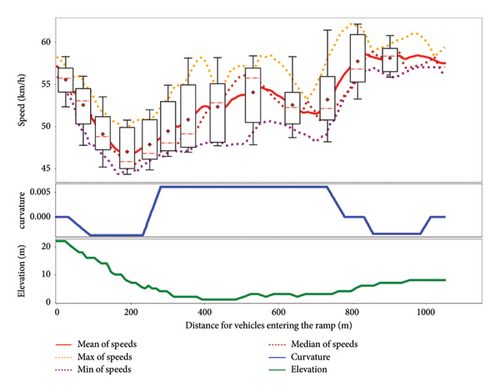
A significant correlation exists between vehicle speed and road curvature. By conducting an in-depth analysis of map data obtained from OpenStreetMap, the road curvature characteristics were successfully modeled. As shown in Figure 2, the speed distribution of multiple vehicles traversing the same ramp reveals a clear trend: vehicles tend to decelerate as road curvature increases. Specifically, the average speed of vehicles on curved sections is approximately 10 km/h lower than on straight segments.
- 2.
The speed variation of vehicles entering and exiting ramps exhibits distinctly different patterns. As illustrated in Figure 2, vehicles enter the ramp at an average speed of approximately 57 km/h, but upon entering the ramp, their speed quickly decreases to around 47 km/h, indicating significant deceleration. In contrast, when exiting the ramp, vehicles begin to accelerate, with their average speed rising back to about 57 km/h. This speed variation is likely influenced by a combination of road curvature and vehicle behaviors during ramp entry and exit, resulting in differing speed fluctuation patterns at various points along the same ramp.
- 3.
There is no evident linear relationship between vehicle speed and road gradient, as shown in Figure 2. Elevation data, collected via the GPS system, reveals that vehicle speeds do not significantly decrease on uphill sections nor notably increase on downhill sections. This phenomenon can likely be attributed to drivers’ tendency to smoothly adjust the throttle and brakes during driving, maintaining a steady speed and mitigating substantial speed fluctuations caused by gradient changes.
- 4.
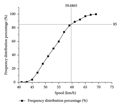
Vehicles frequently surpass the designated speed limit. As an illustrative example, we consider the Yanggao North Road Expressway Interchange Ramp situated at the interchange of Wuzhou Avenue and Yanggao North Road in Shanghai for analysis. The speed limit for this ramp is set at 40 km/h. Figure 3 reveals that upon entering the ramp, over 90% of operating speeds exceed the speed limit, with over 80% surpassing it by 10%. The speed at the 85th percentile of vehicles on the ramp is 59.74 km/h, surpassing the speed limit by 44%. It is evident that speeding constitutes a significant issue for vehicles on this ramp. Consequently, studying the operating speed model of vehicles on ramps becomes imperative to offer guidance for road safety assessment [37].
- 5.
To further investigate the relationships between variables, we analyze the statistical correlation between operating speed and the following factors: ramp curvature, ramp length, ramp gradient, square of ramp curvature, square of ramp gradient, interaction term between ramp gradient and curvature, interaction term between ramp gradient and length, and interaction term between ramp curvature and length using Pearson correlation analysis. The Pearson coefficient analysis results are shown in Table 2. From Table 2, it can be seen that the p value of the correlation coefficient between the curvature of the slope, the square of the slope, the length of the slope, and the interaction term between the curvature and length of the slope and the operating speed of the vehicle is less than 0.05, indicating a significant statistical correlation.
| Ramp gradient | Ramp curvature | Ramp length | Square of ramp gradient | |
|---|---|---|---|---|
| Pearson correlation coefficient with operating speed | 0.312 | −0.33 | 0.539 ∗ | 0.536 ∗ |
| Sig. (p value) | 0.258 | 0.049 | 0.0380 | 0.040 |
| Square of ramp curvature | Interaction term between tamp gradient and curvature | Interaction term between ramp curvature and length | Interaction term between ramp gradient and length | |
| Pearson correlation coefficient with operating speed | −0.055 | −0.043 | −0.32 | −0.025 |
| Sig. (p value) | 0.846 | 0.880 | 0.049 | 0.929 |
- ∗symbol is used to indicate that the correlation coefficient between the variables in question is greater than 0.5. This means that there is a moderate to strong linear relationship between the variables.
Based on the above analysis results, the subsequent models will factor in the influence of ramp curvature, the square of the slope, ramp length, and the interaction term between ramp curvature and length on operating speed.
4.2. Analysis of Speed Variation Trends
This section investigates the fluctuations of vehicle speeds at different positions on the same ramp, employing the K-means method for trajectory clustering to analyze vehicle speed trajectories. Initially, all trajectories on each ramp are aligned based on the ramp entry position. Subsequently, the average velocity for each ramp is calculated to derive the velocity-position trajectory across different ramps. Finally, the Dynamic Time Warping (DTW) algorithm is used to measure the trajectory similarity, which can adjust for time compression and expansion to mitigate the influence of segment length. The Euclidean distances of geometric shape, velocity, and direction are calculated separately and assigned weights of 0.69, 0.23, and 0.08 for aggregation based on entropy weight method. Here, geometric shape refers to the curvature and length of the ramp, velocity refers to the average speed of vehicles traveling at different trajectory points on the ramp, and direction refers to the slope of the ramp. Figure 4 displays the clustering outcomes, which illustrate the trajectory distribution across three distinct clusters, differentiated by red, blue, and green, respectively.
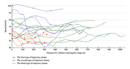
Based on the clustering results, it is observed that operating speed curves of ramps of different lengths exhibit different oscillation patterns. Subsequently, to delve deeper into the driving characteristics of vehicles on various ramps, an examination of operating speed on ramps of different lengths is undertaken, as depicted in Figure 5. Speed curves of distinct colors denote varying lengths of the ramp: (1) When the ramp length is less than 400 m, the operating speed exhibits a clear decreasing trend followed by an increasing trend, with little or no prolonged periods of stable speed driving. (2) When the ramp length is between 400 and 700 m, the operating speed is unstable, showing more fluctuations. (3) When the ramp length exceeds 700 m, vehicles tend to maintain a relatively stable speed during the middle section of the ramp.


5. Methods
5.1. GLM
5.2. GLM With Spatial Correlation Consideration
Given the complex linear combinations of urban expressway ramps, a vehicle’s speed at a specific point is consistently influenced by the states of adjacent trajectory points, including road curvature, speed, and gradient. To address this, we developed a GLM that incorporates spatial correlation using an EMA framework. This method, widely recognized for its effectiveness in capturing trends and fluctuations in time-series data, is equally adept at handling spatially correlated data. In our model, the EMA structure adjusts for distance-based weighting, reflecting the varying impact of trajectory points at different distances on the current speed.
5.3. DNNS
The DNN can discern higher-level and more abstract features, enhancing the model’s ability to generalize and achieve more precise predictions of operating speed curves. Consequently, we introduce the DNNS to predict the short-term operating speed of small passenger cars. This model aims to capture the speed fluctuations of vehicles on urban expressway interchange ramps comprehensively and provide a detailed overview of the speed distribution of vehicles throughout the interchange ramp.
The DNNS takes inputs such as yi,k−1, Hi,k, xi,k, , and xi,k · hi,k, with vi,k−1, as the corresponding output. The meanings of these parameters correspond to those in the “Generalized Linear Model Considering Spatial Correlation.”
6. Results and Application
The trajectory data for interchange ramps on Shanghai urban expressways were acquired in the “Interchange Ramp Data Extraction” section. To calibrate the model, 673 trajectory data are used for model training, while the remaining 301 trajectory data are utilized for model validation. Additionally, considering the distinct driving characteristics on ramps of varying lengths, separate model calibrations were performed for ramp lengths of 0–400 m, 400–700 m, and greater than 700 m.
6.1. Model Calibration
Parameter calibration for both the GLM and the GLMS is executed using the R software. The Markov Chain Monte Carlo (MCMC) sampling method is employed for parameter estimation. The mean values of the estimated model parameters are presented in Table 3, while Table 4 displays the 95% confidence intervals.
| Ramp length (m) | Parameter | 0–400 | 400–700 | > 700 |
|---|---|---|---|---|
| GLM | b0 | 2.47 | 2.93 | 2.60 |
| b1 | 0.002 | −0.001 | −0.01 | |
| b2 | −1.940 | −1.824 | 4.288 | |
| b3 | −0.372 | 0.425 | 0.067 | |
| b4 | 0.0056 | −0.123 | 0.014 | |
| GLMS | b0 | 0.15 | −0.15 | 0.11 |
| b1 | 1.751 | 2.494 | −0.096 | |
| b2 | 3.543 | 7.27 | −0.81 | |
| b3 | −0.476 | −0.123 | −0.125 | |
| b4 | 3.071 | 59.27 | 3.393 | |
| Ramp length (m) | Parameter | 0–400 | 400–700 | > 700 |
|---|---|---|---|---|
| GLM | b0 | (2.38, 2.56) | (2.90, 2.96) | (2.59, 2.61) |
| b1 | (0.001, 0.003) | (−0.001, 0.001) | (−0.011, −0.008) | |
| b2 | (−2.921, −1.130) | (−3.490, −0.174) | (3.036, 5.592) | |
| b3 | (−0.096, 0.843) | (0.351, 0.500) | (0.053, 0.079) | |
| b4 | (0.003, 0.008) | (−0.136, −0112) | (0.011, 0.016) | |
| GLMS | b0 | (0.13, 0.17) | (−0.17, −0.13) | (0.096, 0.12) |
| b1 | (0.817, 2.664) | (0.957, 4.063) | (−0.134, −0.060) | |
| b2 | (3.043, 4.054) | (6.602, 8.268) | (−1.014, −0.629) | |
| b3 | (-0.590, −0.365) | (−0.181, −0.0631) | (0.144, 0.108) | |
| b4 | (1.647, 4.495) | (48.55, 69.62) | (2.5, 4.3) | |
Table 4 indicates that the 95% confidence intervals of GLMS do not encompass zero, signifying the significance of the parameters at a higher significance level. Conversely, the confidence intervals of GLM include zero in fewer instances, suggesting that some parameters of this model lack significance at a higher significance level. GLM assumes independence among operating speeds at different trajectory points during vehicle travel, neglecting the inherent correlation in operating speeds as time series. The significance levels derived from the MCMC sampling estimation underscore the limitations of GLM. In contrast, the GLMS proposed in this study acknowledges and incorporates the spatial correlation in operating speeds, resulting in improved significance in parameter estimation from MCMC sampling.
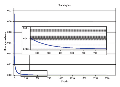
Furthermore, an orthogonal experiment was designed to determine the optimal network structure, and the considered factors along with their respective values are detailed in Table 5. After a series of cross-validation processes, the hyperparameters for DNNS are selected as outlined in Table 6. The loss curve of the DNNS model training, depicted in Figure 6, illustrates the convergence of the value infinitesimally close to the x-axis and the loss value shows 0.0000001, affirming the model’s convergence post-training.
| Model structure | Activation function | Max epochs | Hidden layer | Initial learn rate |
|---|---|---|---|---|
| CNN | RELU | 500 | 32 | 0.001 |
| DNN | Sigmoid | 1000 | 64 | 0.0001 |
| Informer | Tanh | 2000 | 128 | 0.00001 |
| Transformer | — | 5000 | 256 | 0.000001 |
| Parameter | Setting |
|---|---|
| Activation function | RELU |
| Max epochs | 2000 |
| Hidden layer | 64 |
| Model structure | DNN |
| Initial learn rate | 0.0001 |
| Loss function | MSE |
| Optimizer | SGD |
6.2. Model Validation
The established models are employed to predict the operating speeds of 10 additional ramps that were not involved in parameter calibration. These predicted results are then compared with the actual operating speed data obtained from natural driving experiments. For evaluation purposes, R2, MAPE, and MSSE are calculated and presented in Table 7, which shows the maximum MAPE for GLMS to be 10.80%, and the maximum MAPE for GLM to be 24.12%. This highlights the significance of considering the dependence of operating speeds between vehicle trajectory points to achieve accurate speed prediction on urban expressway interchange ramps. On the other hand, the maximum MAPE for DNNS is 9.14%, indicating that DNNS demonstrates higher accuracy in predicting operating speed compared to GLM and GLMS for these 10 ramps. In most cases, the predictive accuracy of DNNS is approximately 95%, as revealed by the MAPE indicator. Moreover, the average R2 and MSSE for DNNS are 0.81 and 0.92, respectively. GLM, GLMS and DDNS had chi-square test significances (Sig.) greater than 0.05, indicating acceptance of the null hypothesis, suggesting that there is no significant difference between the predicted operating speeds and the actual measurements. These values indicate that DNNS successfully captures the relationship between operating speed and the geometric characteristics of urban expressway interchange ramps, effectively reflecting the speed fluctuations of vehicles on the ramp.
| No. | Length of ramp | GLM | GLMS | DNNS | |||||||||
|---|---|---|---|---|---|---|---|---|---|---|---|---|---|
| R2 | Sig. | MAPE | MSSE | R2 | Sig. | MAPE | MSSE | R2 | Sig. | MAPE | MSSE | ||
| m | — | — | % | m/s | — | — | % | m/s | — | — | % | m/s | |
| 1 | 209 | 0.15 | 0.25 | 5.13 | 0.75 | 0.60 | 0.25 | 5.61 | 0.91 | 0.87 | 0.86 | 3.18 | 0.81 |
| 2 | 280 | 0.44 | 0.25 | 6.10 | 1.31 | 0.74 | 0.65 | 9.94 | 3.92 | 0.88 | 0.88 | 3.07 | 0.76 |
| 3 | 389 | 0.32 | 0.24 | 17.02 | 8.29 | 0.79 | 0.24 | 10.75 | 3.68 | 0.76 | 0.72 | 4.53 | 1.13 |
| 4 | 418 | 0.33 | 0.24 | 34.69 | 25.9 | 0.67 | 0.35 | 10.29 | 5.21 | 0.89 | 0.52 | 9.14 | 1.55 |
| 5 | 243 | 0.26 | 0.24 | 12.97 | 3.52 | 0.79 | 0.24 | 10.80 | 2.46 | 0.71 | 0.51 | 3.60 | 0.74 |
| 6 | 315 | 0.20 | 0.24 | 24.12 | 9.85 | 0.80 | 0.24 | 4.10 | 0.43 | 0.72 | 0.55 | 2.42 | 0.47 |
| 7 | 1064 | 0.59 | 0.25 | 21.04 | 11.2 | 0.77 | 0.25 | 9.71 | 2.47 | 0.80 | 0.06 | 8.59 | 1.37 |
| 8 | 609 | 0.22 | 0.25 | 14.22 | 12.7 | 0.66 | 0.25 | 5.97 | 2.32 | 0.94 | 0.73 | 1.50 | 0.35 |
| 9 | 757 | 0.82 | 0.25 | 7.54 | 2.85 | 0.82 | 0.25 | 7.39 | 2.31 | 0.73 | 0.55 | 4.91 | 0.86 |
| 10 | 667 | 0.69 | 0.24 | 11.01 | 4.31 | 0.88 | 0.24 | 5.27 | 1.14 | 0.84 | 0.58 | 5.17 | 1.04 |
| Avg | 495 | 0.40 | 0.25 | 15.38 | 8.07 | 0.75 | 0.30 | 7.98 | 2.49 | 0.81 | 0.60 | 4.61 | 0.91 |
The velocity fluctuation curve predicted by the established models is depicted in Figure 7, where the results from the Transformer model are also included. The Transformer model has recently garnered attention and achieved some success in time series prediction. As illustrated in Figure 7, in comparison to the GLM, the GLMS, and the Transformer model, the DNNS model exhibits higher prediction accuracy and better reflects the fluctuation trend of vehicle speed on the ramp.
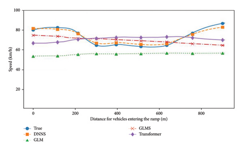
Overall, the estimation results of the DNNS showcase superior robustness and generalization performance in accurately predicting the short-term operating speed for compact passenger vehicles on urban expressway interchange ramps. In other words, both the DNNS and the GLMS exhibit certain advantages over the GLM. Recognizing the dependence of operating speeds between vehicle trajectory points is essential for accurate speed prediction in practical scenarios. The DNNS demonstrates distinct advantages over the GLM and the GLMS, with the DNN significantly outperforming the GLM in capturing the speed fluctuations of vehicles on ramps.
6.3. Model Application
The developed model serves as a valuable tool for assessing road safety, specifically in reviewing the speed uniformity of vehicles on ramps. In cases where significant fluctuations in vehicle speed occur, it is advisable to devise precise and targeted speed control measures.
As depicted in Figure 7, the DNNS model adeptly predicts the short-term operating speed of compact passenger vehicles traversing an interchange ramp. The model’s calculations indicate that the speed of vehicles entering the ramp is 80 km/h. However, within a distance range of 200–400 m along the ramp, the operating speed decreases to approximately 60 km/h and stabilizes at this level. Subsequently, as vehicles cover a distance of 600–800 m along the ramp, the operating speed exhibits an upward trend. The resulting operating speed curve enables road managers to accurately anticipate speed fluctuations on ramps and develop more precise speed control measures based on both the position and magnitude of speed variations [42].
7. Conclusions and Discussion
This study utilizes vehicle trajectory data from SNDD to develop three models—GLM, GLMS, and DNNS—by comprehensively considering the effects of road alignment and spatial correlation on urban expressway ramps. The GLM assumes that the operating speeds at different trajectory points are independent, focusing solely on road alignment. In contrast, the DNNS and GLMS models account for the influence of spatial correlation on vehicle operating speeds.
The trajectory data, extracted from our natural driving experiments, are employed for the calibration and validation of model parameters. The predictive outcomes reveal that the DNNS consistently surpasses the GLM and the GLMS, attaining an impressive prediction accuracy of approximately 95% and showcasing superior robustness and generalization capabilities. These results unequivocally underscore the significance of accounting for spatial correlation in constructing operating speed prediction models for urban expressway interchange ramps.
The DNNS adeptly calculates vehicle operating speeds at diverse spatial points across the entire interchange ramp, accommodating different entry speeds and delivering a heightened level of granularity. This precision furnishes valuable insights for road safety assessments, empowering highway engineers to evaluate the safety implications of specific geometric attributes of urban expressway interchange ramps.
Despite its advantages, the DNNS model, when compared with GLM and GLMS, still exhibits certain inherent limitations, particularly its high computational complexity and challenges in its interpretability. Further research aimed at addressing these constraints is expected. In addition, this study focuses solely on predicting vehicle speeds within the ramps, excluding the merging and diverging areas. However, speeds in these regions also influence the speeds on the ramp. Future studies should also investigate vehicle behaviors in the merging and diverging zones of the ramp.
Additionally, this study employs EMA to explore the significance of spatial correlation in predicting operating speeds. With the increasing availability of data, future research could investigate the integration of more advanced spatiotemporal analysis techniques to replace EMA, further enhancing model performance and extending its applicability. This advancement could provide valuable insights and optimizations for speed decision-making in autonomous vehicles.
Conflicts of Interest
The authors declare no conflicts of interest.
Funding
This research was funded by the National Natural Science Foundation of China (NSFC, Grant no. 71871161) and National Key Research and Development Program of China (Grant no. 2019YFB1600703).
Open Research
Data Availability Statement
The data that support the findings of this study are available on request from the corresponding author. The data are not publicly available due to privacy or ethical restrictions.


