1. Introduction

In recent years, satellite remote sensing technology has made remarkable progress, resulting in the creation of video satellites such as “Jilin-1” [1]and “SkySat-1” [2]. These satellites have successfully addressed the shortcomings of conventional satellites in capturing dynamic information about moving objects, enabling real-time, uninterrupted observation of vast ground areas. This advancement has immense significance in both theoretical and practical domains, especially in intelligent transportation and urban planning. Nowadays, the research of intelligent transportation systems (ITSs) is more and more extensive, and the acquisition of traffic flow information is an essential basis for the construction of ITS [3]. Traditional methods of traffic data collection, including coil detectors [4], Lidar [5], and floating vehicles [6], have been constrained by their limited coverage area and prolonged data aggregation periods. For instance, inductive loop detectors require extensive infrastructure installation and are often costly to maintain, while LiDAR, despite its accuracy, can be limited by line-of-sight constraints and high implementation costs. Floating car systems provide valuable travel time data but are subject to sampling limitations and delays due to the random nature of moving vehicles. These methods are increasingly inadequate for the demands of large scale and efficient traffic monitoring development. Satellite video has a large field of view and can quickly obtain extensive traffic information. The traffic flow parameter extraction method based on satellite video has gradually become a hot spot in traffic information collection research. However, due to satellite video’s low resolution and complex background, it is difficult to achieve accurate and effective tracking of small targets such as vehicles [7]. The pixel size of vehicles is usually relatively small, so the amount of information stored is little [8]. These factors introduce challenges in terms of target detection and tracking accuracy, which are critical for the reliable extraction of traffic flow parameters. Researchers commonly use target tracking algorithms, which are mainly divided into generative and discriminative [9]. The generative target tracking algorithm models the statistical features of the target and the background and then uses these models to estimate the position of the target in the new frame. It does not require prelabeled training data and has certain adaptability to the appearance changes of the target. Luo, Liang, and Wang [10] used the Shi-Tomasi corner detection algorithm to detect vehicle key points in video and used optical flow method to track vehicle key points to achieve vehicle tracking, but the tracking accuracy was not high. Wang [11] used the template matching method in the generative algorithm to track multiple vehicles in remote sensing satellite videos. However, this approach exhibits several limitations, including a protracted traversal time across the entire area of interest, an inability to differentiate between multiple vehicles with similar characteristics, and a heightened sensitivity to conditions of occlusion. It cannot be really applied to the actual traffic scenario.

Compared with the generative target tracking algorithm, the discriminative algorithm takes both background and target as training samples to train the tracker and treats target tracking as a binary classification problem of background and target, which has more advantages in tracking accuracy and robustness. In 2010, Bolme et al. [12] first applied correlation filtering theory to target tracking and proposed a MOSSE tracking algorithm. However, it was not until 2018 that kernelized correlation filter (KCF) was not applied to target tracking in satellite video [13]. Henriques et al. [14] formally proposed the target tracking framework of correlation filtering, and KCF [15] is one of the most representative works in the target tracking algorithm of correlation filtering. In order to realize vehicle tracking in satellite video, Wang et al. [7] proposed a WTIC algorithm, which uses correlation filter CSK to track vehicles in satellite videos and evaluates the correlation filtering algorithm using two criteria: success rate and precision. But when the target is partially or completely blocked by obstacles in the video, the tracking performance of the CSK algorithm will decline. Xuan et al. [16] proposed a novel tracking algorithm (CFME) based on correlation filter and motion estimation, combined with Kalman filter and motion trajectory averaging, which effectively solves the problem of tracking moving targets in satellite video and improves tracking accuracy, and effectively handled tracking failures caused by occlusion. Xuan et al. [17] presented a rotation adaptive correlation filtering algorithm to solve the problem of target scale change in satellite video. Although these studies effectively solve the problem of target occlusion and multi-scale vehicle, they do not consider the problem of tracking drift or tracking jump caused by the small size, low resolution and fuzzy features of the vehicle in satellite video, as well as the interference of other vehicles or other objects with similar shape to the vehicle. But the multifeature fusion strategy can combine the image features of different scales to provide multilevel and multiscale semantic information and enhance the recognition ability [18]. In addition, it can obtain the global information in the video, reduce the loss of information [19], make the model retain more detailed information, reduce the misjudgment of the target, and effectively reduce the occurrence of tracking drift and tracking jump. This strategy can effectively improve the robustness and adaptability of the algorithm [20, 21]. Considering that vehicle features in satellite video are not obvious, Liu et al. [22] combined HOG features, LBP features, and grayscale features to effectively describe the contour and shape information of the target. This method improves the tracking performance of the tracker. Chen et al. [23] adopted spatial spectral feature fusion to enhance the representation of objects, prevent tracking drift, and enhance the accuracy and robustness of KCF. Zhang et al. [24] designed a multifeature fusion strategy, which significantly enhanced the representation power of target tracking by combining a variety of manual features with equal weights and fusing them with depth features with adaptive weights. Yet they do not take into account and reflect interference from similar or adjacent objects to vehicle tracking. With the development of deep learning, convolutional neural network CNN and Transformer and other architectures have been applied in the field of target tracking. However, satellite video is characterized by large data volume, low resolution, smaller foreground target size, fewer features, and similar to the environment. Reference [25] proposed a tracking algorithm based on SiamTM of CNN network, which can be well applied to moving targets in satellite video, but this algorithm can only track a single target, and the speed is lower than that of other types of siamese network. Meanwhile, when there are interfering objects with similar characteristics near the target search area, the tracking may drift or fail in some frames of the video. Reference [26] proposed a satellite video multitarget tracking algorithm combining Transformer and the attention mechanism, which improves the tracking performance by enhancing the features of small targets and improving the association strategy. The traditional trackers based on deep learning cannot be directly applied to satellite video tracking. It is mentioned in Ref. [27]that CNN network has a strong feature extraction ability, but the global information obtained is limited, and it is difficult to accurately track the target when obstacles are obstructed. Reference [28] emphasized that convolutional neural networks are prone to lose context information outside the convolution kernel perception region. Transformer’s attention mechanism can acquire more context information, but its ability to acquire local features is too weak, so the tracking effect of small targets is poor [29]. However, the algorithm still needs to solve the limitations of real-time and target-specific tracking. The tracking accuracy of deep learning algorithm has been improved, but the real-time processing ability of the algorithm is still limited, especially the tracking effect of specific targets is not ideal, and a large amount of data is required for training. In addition, deep learning algorithms rely heavily on high-quality and diverse training data, and their adaptability to new scenarios needs to be further strengthened.

The organization of the paper is as follows: Section 1 is the introduction. The section had depicted the research background, related problems, and related work of this paper. Section 2 is the proposed algorithm. The section had depicted research problem, the principle of the proposed algorithm, multifeature fusion method, and Kalman filter principle. Section 3 is experimental results and discussion. The section had compared the performance of the proposed method with other mainstream algorithms in tracking accuracy and success rate. Section 4 is the traffic flow parameter exaction. The section had depicted the principle of the virtual detection line method and discussed the experiments of traffic extraction under different traffic conditions, such as smooth and congested traffic.

2. Vehicle Tracking Based on Improved KCF

2.1. Improved KCF Vehicle Tracking Algorithm

2.1.1. Problems

After carefully examining the satellite footage and the characteristics of the target vehicle, it has been conclusively determined that there are two major obstacles to effectively tracking a moving vehicle.

• 1.

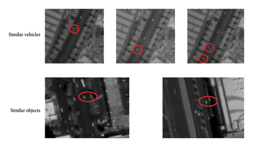
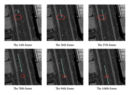
  Objects with similar characteristics to vehicle targets in complex backgrounds will increase the discrimination error of the tracker, making the tracker track the wrong target, see Figure 1.

• 2.

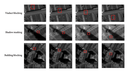
  Obstructions such as buildings and trees can cause shadows that disrupt tracking. These can result in tracking stopping completely, as shown in Figure 2.

2.1.2. Principle of the Improved KCF Vehicle Tracking Algorithm

The KCF based on the discrete Fourier Transform (DFT) [30] framework estimates the target position by calculating the correlation between the target template and the searched image. It transforms the target tracking problem into the calculation and updating process of the correlation filter, which has been proven to be a simple and effective tracking method. The KCF has high computing power, which can quickly calculate the correlation between the template and the search image to achieve fast target tracking. However, due to the fact that KCF tracks the target through the correlation between the template and the search image, the changed appearance of the target makes the learned template inconsistent, which leads to the decline of tracking precision and the problem of vehicle tracking loss occuring in the case of the KCF. Therefore, the Kalman filter is used to predict and estimate the position and state of the vehicle when the vehicle is blocked. Thus, the vehicle trajectory prediction can be realized under the occlusion condition. In the face of vehicle tracking errors caused by adjacent objects with similar vehicle features in complex backgrounds, multifeature fusion is introduced after feature extraction by KCF to improve the discriminant ability of the algorithm. According to the abovementioned improvements, the flow of the vehicle tracking algorithm with KCF improved in this paper is shown in Figure 3.

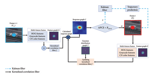
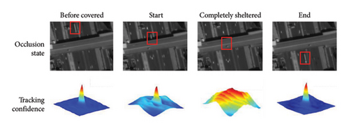
The KCF’s average peak correlation energy (APCE) can measure the confidence of target tracking by evaluating the degree of fluctuation in the response graph. It can also determine whether a vehicle is obstructed by analyzing the APCE peak value and the R_APCE threshold value. Figure 4 illustrates how the response diagram changes as a vehicle passes through the viaduct construction. The features are apparent, and the APCE value is high when the vehicle is not obstructed. As the vehicle enters the viaduct, the APCE value drops, but the tracker can still determine the vehicle’s position from the slightly fluctuating response graph. However, when the vehicle is completely obscured, the response graph fluctuates wildly without any clear peak. As the ideal response graph is a two-dimensional Gaussian function, if the actual response graph fluctuates greatly and the APCE value is small, the tracking results cannot be considered reliable.

This algorithm uses a frame image from a video as input to identify the target position to track, represented by a rectangular box. The output predicts the target’s position coordinates and the size of its rectangular box in subsequent frames. For instance, in Figure 3, consider frames t − 1 and t. The target box’s position in frame t − 1 is P_t−1, and its position in frame t is P_t. The vehicle tracking process is divided into two situations depending on whether the vehicle is obscured.

In the first case, if the peak value of APCE exceeds the R_APCE threshold, the vehicle is not obstructed, and the KCF is utilized for tracking. The following steps outline the specific procedure:

• •

  Step 1: the search area for frame t is determined by examining the neighboring area of the previous target frame P_t−1 from frame t − 1.

• •

  Step 2: features are extracted and fused from the search area on the t − 1 frame. Then, the obtained feature map X is convoluted with the set correlation filter F to obtain the response graph C. The position coordinates of the APCE peak on the response graph C are calculated to obtain the tracking results of the t frame.

• •

  Step 3: using the current tracking results, the image is cropped with the target as the center, and the feature map Z is obtained after feature extraction, and the feature map Z is solved by the followin g minimization formula for the associated filter f.

  $$ ()
  $$ ()

•  

  In Formula (1a), α is the weight vector of the KCF. ⊙ is the eigenvector of the training sample. y_i is the corresponding target label. x_i represents the dot product of the matrix, λ is the regularization parameter to control overfitting, and the initial value of λ in the experiment is 0.0001. In Formula (1b), • denotes the circular convolution operation, and Y denotes the 2D Gaussian distribution.

• •

  Step 4: the above steps should be followed for each frame of the video in order to calculate the target tracking results and obtain the updated relevant filter.

The second case is that when the peak value of APCE is less than the threshold R_APCE, the vehicle is occluded. The Kalman filter is used for occlusion detection to accurately predict and estimate the position and state of the vehicle in the next frame. The KCF is stopped until the peak value of APCE is greater than the threshold R_APCE, the occlusion is over, and the tracking results of the Kalman filter are used to update the parameters of the KCF for continuous tracking. The specific process of the Kalman filter occlusion detection is as follows:

• •

  Step 1: determine the target search area of frame t through the local adjacent region of the target frame P_t−1 of frame t − 1. Conduct feature extraction and multi-feature fusion on the obtained search area on frame t − 1, and perform cyclic convolution operation on the obtained feature map X and the set correlation filter F to obtain the response graph C.

• •

  Step 2: determine whether the object is occluded by comparing the peak value of APCE in the response graph with the size of the threshold R_APCE, which is set to 18 after many tests in the experimental dataset. When the APCE value in the response graph is less than the threshold R_APCE, the vehicle is determined to be in a state of occlusion. The Kalman filter is enabled for occlusion detection because the target position calculated by the KCF is not accurate. The prediction result of the Kalman filter is output as the tracking result of the target.

• •

  Step 3: when the peak value of APCE in the response graph is greater than the threshold R_APCE, it is determined that the occlusion of the vehicle is over. The final prediction result of the Kalman filter is used as the input to update the parameters of the KCF, and the vehicle features are extracted and compared with the features stored in the KCF to measure the similarity and connect and correct the vehicle trajectory, to realize the continuous tracking. Otherwise, proceed to Step 2.

2.1.3. Multifeature Fusion

In order to cope with the tracking error problem caused by the proximity of similar targets, this paper uses grayscale features and CN color features to assist the HOG features used to train the KCF, respectively. Finally, adaptive fusion is performed to obtain the target response graph to determine the target location. The response graph calculation method is shown in the following formula:

$$ ()

$$ ()

$$ ()

$$ ()

$$ ()

In Formula (2a), $$ is the Gaussian kernel function transformed by a DFT to measure the similarity between two samples x^′ and x. F stands for DFT. ∂ is the bandwidth parameter of the kernel function, which determines the sensitivity of the similarity. $$ is the square of the Euclidean distance between the two samples. In Formula (2b), $$ represents the feature vector. $$ is the Gaussian kernel function. I is the identity matrix. y is the target label vector, and $$ is the value after the DFT. In Formulas (2c)–(2e), $$, $$, and $$ represent the Gaussian kernel function between the target sample of HOG feature, gray feature, and CN color feature and the candidate region of the next frame, respectively. $$, $$, and $$ represent the feature vectors of HOG feature, gray feature, and CN color feature after DFT in correlation filter respectively. Those feature vectors can be calculated by Formula (2b). ⊙ represents the dot product between matrices. F⁽⁻¹⁾ represents the discrete Fourier inverse transform; f_HOG(z), f_GRAY(z), and f_CN(z) represent the response graphs of corresponding features, respectively.

Through the response graph of f_HOG(z), f_GRAY(z), and f_CN(z) in Formulas (2c)–(2e), we can obtain the value f(i, j) of each point in the corresponding graph, including the maximum value f_max and the minimum value f_min. Finally, according to the size M × N of the response graph, we can use Formula (3) to calculate the value of the response graph APCE of f_HOG(z), f_GRAY(z), and f_CN(z), respectively.

$$ ()

APCE has two functions, the first is to judge the condition of whether the target is blocked and the second is to calculate the fusion weight of each feature response graph. In Formula (4a), f_M is calculated by f_max and APCE, and the mean of the sum of f_M of all previous frames is normalized according to Formula (4b) to obtain ξ. The purpose of that is to make the model pay more attention to the relative differences between features rather than the numerical size, which helps the model learn the key features to distinguish similar objects, and dynamically adjust the feature weights. The tracking system can adaptively select the features that are most suitable for the current environmental conditions and reduce the interference of similar objects.

$$ ()

$$ ()

Through the calculation results of Formula (4b), we can get the e corresponding to HOG feature, grayscale feature, and CN color feature and thus get the fusion weight ϕ_HOG, ϕ_GRAY, and ϕ_CN of each feature, respectively. The fusion weight calculation formula is as follows:

$$ ()

$$ ()

$$ ()

Finally, according to Formula (6), the final response graph f(z) can be obtained by weighted response graphs of the three features. The multifeature fusion process in this paper is shown in Algorithm 1.

$$ ()

Algorithm 1: Multifeature fusion.
•  

  Input:

•  

  n: number of processed frames;

•  

  Output:

•  

  f(z)_k: the final feature response graph Z at frame k

•  

  / ^∗ Initialize the fusion weights and response graphs/:

•  

  f1_k ← A list of f_{M_HOG}(z)_k used to store;

•  

  f2_k ← A list of f_{M_GRAY}(z)_k used to store;

•  

  f3_k ← A list of f_{M_CN}(z)_k used to store;

•  

  for k in n:

•  

   /^∗KCF obtains the features of the target region and the response graph for each feature/:

•  

   $$, $$, $$ ← The feature vectors are calculated by Formulas (2a)–(2b);

•  

   f_HOG(z)_k ← f_HOG(z)_k is calculated by using Formula (2c);

•  

   f_GRAY(z)_k ← f_GRAY(z)_k is calculated by using Formula (2d);

•  

   f_CN(z)_k ← f_CN(z)_k is calculated by using Formula (2e);

•  

   /^∗Calculate the APCE value for each response graph and the valuef_Mof the product of the APCE value and the maximum value in the response graph/:

•  

   APCE_HOG(z)_k ← Using Formula (3);

•  

   APCE_GRAY(z)_k ← Using Formula (3);

•  

   APCE_CN(z)_k ← Using Formula (3);

•  

   f_{M_HOG}(z)_k ← Using Formula (4a);

•  

   f_{M_GRAY}(z)_k ← Using Formula (4a);

•  

   f_{M_CN}(z)_k ← Using Formula (4a);

•  

   f1_k append f_{M_HOG}(z)_k ← The f_{M_HOG}(z)_k of all previous frames is stored;

•  

   f2_k append f_{M_GRAY}(z)_k ← The f_{M_GRAY}(z)_k of all previous frames is stored;

•  

   f3_k append f_{M_CN}(z)_k ← The f_{M_CN}(z)_k of all previous frames is stored;

•  

   /^∗Normalize the me an value of all previous framef_M/:

•  

   ξ_HOG(z)_k ← Using Formula (4b);

•  

   ξ_GRAY(z)_k ← Using Formula (4b);

•  

   ξ_CN(z)_k ← Using Formula (4b);

•  

   /^∗Calculate the weight of each feature by usingξ/:

•  

   ϕ_HOG(z)_k ← Using Formula (5a);

•  

   ϕ_GRAY(z)_k ← Using Formula (5b);

•  

   ϕ_CN(z)_k ← Using Formula (5c);

•  

   /^∗Calculate the final feature response graph Z/:

•  

   f(z)_k = ϕ_HOG(z)_kf_HOG(z)_k + ϕ_GRAY(z)_kf_GRAY(z)_k + ϕ_CN(z)_kf_CN(z)_k

•  

  Returnf(z)_k

2.1.4. The Algorithm Principle of the Kalman Filter

The Kalman filter is an optimal linear filter under the minimum mean square error criterion. Since the vehicle motion in the adjacent frames of satellite video images is very slow and approximately uniform, the target can be tracked by using the Kalman filter. The state and observation formulas of the Kalman filter system can be written as Formulas (7a) and (7b).

$$ ()

$$ ()

In Formulas (7a) and (7b), X_k and X_k−1 are the state vectors of the system at time k and k − 1. The observation vector $$, which represents the observed target position at moment k. φ_x,k−1 is the state transfer matrix of the system and H_k is the observation matrix of the system. Since the time between every two frames is very short, it can be assumed that moving objects such as vehicles are in uniform linear motion, so the matrix φ_x,k−1 and H_k can be represented according to Formulas (8) and (9), respectively. Q_k−1 and R_k represent the process noise covariance matrix and the observation noise covariance matrix respectively. The calculation formulas of Q_k−1 and R_k are shown in Formulas (10) and (11). In this system, the state vector X_k is set to $$, where x_sk and y_sk are the horizontal and vertical positions of the target at the moment k and Δx_k and Δy_k are the horizontal and vertical velocities of the target at the moment k.

$$ ()

$$ ()

$$ ()

$$ ()

The trajectory prediction using the Kalman filter described above is shown in the following:

$$ ()

$$ ()

$$ ()

$$ ()

$$ ()

In Formulas (12a)–(12e), $$ refers to the state estimate at time k + 1 given state $$ at moment k. P_k+1,k represents the updated state estimate covariance matrix at moment k + 1. P_k represents the state estimation covariance matrix at moment k. K_k+1 is the Kalman gain that determines the weigh between the observed value and the predicted state. $$ is the optimal state estimate of the system output. Y_k+1 represents the observed target position at moment k + 1. P_k+1 represents the final state estimate covariance matrix at time k + 1. The initial state estimation covariance matrix P₀ is initialized with random data that is not 0. The Kalman filtering process is shown in Algorithm 2.

Algorithm 2: Kalman filter.
•  

  Input:

•  

  n: number of processed frames;

•  

  Output:

•  

  the new position at frame k;

•  

  Y ← A list of target position used to store;

•  

  for k inn:

•  

   Y_k ← the target position in frame k from KCF, Y_k corresponds to the position of the maximum value in the response diagram;

•  

   R ← the APCE value of the response graph in frame k from KCF, R is calculated using Formula (3);

•  

   if k =  = 1then:

•  

    /^∗Initialize the Kalman filter/

•  

    φ ← φ is calculated by using Formula (8);

•  

    H_k ← H_k is calculated by using Formula (9);

•  

    Q_k ← Q_k is calculated by using Formula (10);

•  

    R_k ← R_k is calculated by using Formula (11);

•  

    R_APCE ← The size of R_APCE in the paper is 18;

•  

    P₀ ← The initial state estimation covariance matrix of Kalman filter;

•  

    Y append Y₁ ← Y[0] = Y₁;

•  

   ReturnY₁ ← Y₁ is the new position at frame 1;

•  

   else k > 1 then:

•  

    ifR < R_APCEthen:

•  

     $$ = Y[k − 2] or Y_k−1;

•  

     $$ ← The state estimation is calculated by Formula (12a);

•  

     P_k,k−1 ← The state estimate covariance matrix is updated using Formula (12b);

•  

     K_k ← The Kalman gain is calculated by equation (12c);

•  

     P_k ← The frame k final state estimate covariance matrix using Formula (12e);

•  

     $$ ← The optimal state estimate of the system output is calculated by Formula (12d);

•  

     Y append $$; ← Y[k − 1] = $$;

•  

     Return$$ is the new position at frame k;

•  

    else R > R_APCEthen:

•  

     Y append Y_k ← Y[k − 1] = Y_k;

•  

     ReturnY_k ← Y_k is the new position at frame k;

3. Results and Discussion

3.1. Experimental Data

The experimental data were obtained from panchromatic and multispectral color videos captured by Jilin-1 and Skysat-1 video satellites. In order to verify the feasibility of the tracking method proposed in this paper, according to the requirements of the experiment, a dataset for the experiment was made by intercepting similar targets and video regions under the occlusion condition. The vehicle labeling of this dataset selected moving vehicles. In order to ensure the accuracy of the data, the actual location of the vehicle target was marked manually.

3.1.1. Proximity Similar Target Tracking

Figure 5 shows the tracking of two vehicles in close proximity at frames 36, 348, and 512 when the vehicles are in a dense area or some of them are traveling at a small distance.

3.1.2. Obscured Target Tracking

Figure 6 shows the tracking of the vehicle when it is partially and completely obscured by two types of obstacles caused by signage and overhead bridges.

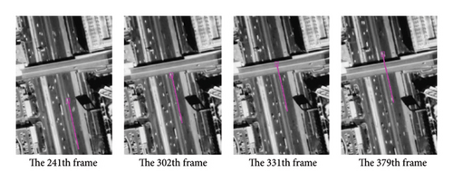
In Figure 6(a), there are two minor signs that are blocking part of the target vehicle. The multifeature fusion method enables the tracker to adapt to minor feature changes to a certain extent. Figure 6(b) shows the vehicle completely obstructed when it reaches the bottom of the viaduct, with the obstruction lasting for a longer time. The vehicle’s trajectory in Figure 6(b) demonstrates that the tracker can predict the driving trajectory at the bottom of the viaduct using the Kalman filter, thus allowing for successful tracking of the occluded target.

3.2. Comparative Experiments on Vehicle Tracking

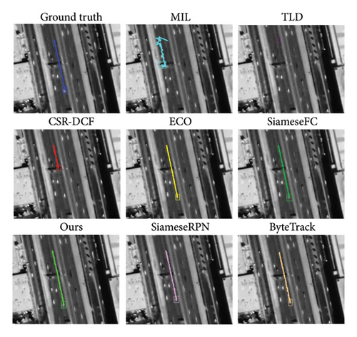
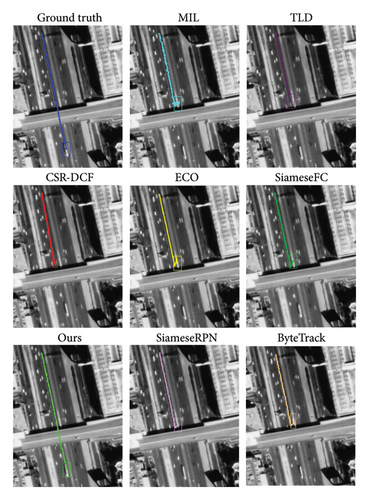
In order to verify the effectiveness of the proposed method, the method was compared with MIL [31], TLD [32], CSR-DCF [33], ECO [34], SiameseFC [35], SiameseRPN [36], and ByteTrack [37]. These algorithms were used to develop experiments and visualize trace trajectories in the experimental dataset.

Figure 7(a) shows the tracking of various algorithms when the vehicle target is partially obscured, where the MIL algorithm cannot accurately locate the vehicle target. ECO, SiameseFC, SiameseRPN, ByteTrack, and the algorithm presented in this paper can track partially obscured vehicle targets normally. Figure 7(b) shows the tracking of various algorithms when the vehicle target is completely obscured, where MIL, TLD, CSR-DCF, SiameseFC, SiameseRPN, and ByteTrack cannot continue tracking when the vehicle target is completely obscured. In this paper, Kalman filter is used for trajectory prediction. This method overcomes the problem of vehicle tracking loss caused by occlusion by accurate estimation and prediction of vehicle position and state.

In this paper, precision and success rate [14] were used to quantitatively evaluate the effectiveness of the proposed method and other mainstream methods in satellite video moving vehicle tracking. Precision is the percentage of the total number of frames in which the Euclidean distance between the prediction and actual frames is less than the predetermined threshold, as calculated by Formulas (13a) and (13b). Success rate is expressed by the overlap between the real target box marked manually and the target box tracking the predicted result. The calculation method of overlap is shown in Formula (14).

$$ ()

$$ ()

$$ ()

In Formulas (13a) and (13b), (x₁, y₁) and (x₂, y₂) represent the coordinates of the center point of the actual box and the prediction box, respectively; d represents the Euclidean distance between the center point of the prediction box and the center point of the actual box; S represents the number of video frames whose Euclidean distance is less than the threshold; and T represents the total number of video frames. In Formula (14), box_p represents the area of the target frame of the tracking result, box_g represents the area of the actual marked frame, ∪ represents the union of the two, and ∩ represents the intersection of the two.

Table 1 shows the comparison results of different tracking algorithms in terms of tracking accuracy, success rate, and FPS. Although the MIL algorithm has low tracking accuracy and success rate, its FPS value is relatively high, which may be due to its low algorithm complexity. The tracking accuracy and success rate of TLD algorithm and CSR-DCF algorithm are improved, but the FPS value is not significantly improved, which may be due to the computational complexity of the algorithm itself. The ECO, SiameseFC, SiameseRPN, and ByteTrack algorithms also showed good FPS performance while improving tracking accuracy and success rate. By adopting efficient feature extraction and tracking strategies, these algorithms can not only maintain high tracking performance but also meet the needs of real-time processing. On the basis of ensuring tracking accuracy and success rate, the proposed method achieves 86.74% tracking accuracy and 79.96% success rate by optimizing algorithm structure and introducing efficient calculation strategy, while maintaining 30.51 FPS value. The results show that the proposed method not only has advantages in tracking performance but also has excellent performance in real-time processing ability, which is suitable for the application scenarios that require tracking speed.

Table 1. Comparison of tracking results.

Tracking method	Precision (%)	Success rate (%)	FPS (f/s)
MIL	25.60	27.82	12.50
TLD	41.60	37.82	3.34
CSR-DCF	39.40	36.80	32.72
ECO	63.15	58.75	22.50
SiameseFC	71.77	64.50	31.03
SiameseRPN	77.56	70.72	27.27
ByteTrack	84.29	78.14	30.58
Proposed	86.74	79.96	30.51

In order to more intuitively represent the tracking performance, we plotted the precision plot and success rate plot under different thresholds, as shown in Figures 8 and 9, respectively. In the precision plot shown in Figure 8, the precision curve visually shows the distance change between the tracking result and the actual value. In this graph, the vertical axis represents accuracy, that is, the percentage of the IoU of the predicted bounding box versus the real bounding box that exceeds the set threshold; The horizontal axis represents the different IoU thresholds that are artificially set. It can be clearly seen from Figure 8 that with the increase of IoU threshold, the accuracy curve of the proposed method always remains at a high level, which is better than other comparison algorithms, especially in the range of medium IoU threshold.

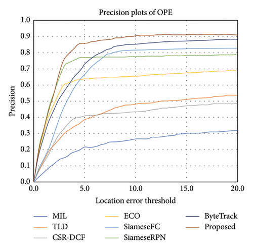
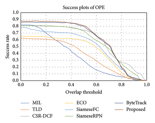
Figure 9 shows the success rate plot, where the horizontal axis represents the artificially set threshold of conformity rate, that is, the percentage of distance between the predicted target center and the real target center that is less than or equal to the set threshold. The vertical axis shows the tracking success rate. It can be observed from Figure 9 that the success rate of the proposed method is higher than that of the comparison algorithm under different distance thresholds, especially under small distance thresholds, and this advantage is more prominent, which shows the superiority of the proposed method in accurately tracking vehicle position.

Based on the results of Figures 8 and 9, it can be concluded that the vehicle tracking method proposed in this paper is significantly superior to other algorithms in terms of accuracy and success rate, which is mainly attributed to the improvement of the algorithm’s feature representation and learning framework so that the tracker can track the vehicle more accurately and stably.

4. Traffic Flow Parameter Exaction

4.1. Traffic Flow Extraction Method

Traffic flow is usually the number of traffic participants passing through a certain section of a road in a unit time. In this paper, a virtual detection line [38] was used for traffic flow extraction, and the moving vehicles passing through the virtual detection line were counted. The principle of it is shown in Figure 10.

Figure 10(a) shows the superimposed results of two frames when the virtual detection line is not passed, Figure 10(b) shows the superimposed results of two frames before and after the vehicle passes the virtual detection line, and Figure 10(c) shows the results after the vehicle target has completely passed the detection line, where A and B represent the two endpoints of the virtual detection line, D and C subtables represent the center of the vehicle target detection frame, and the counting of the vehicle target can be realized when the line DC intersects with the virtual detection line AB.

When line AB intersects line CD, 5 vectors including $$, $$, $$, $$, and $$ are obtained. If centered at point A, the vector $$ is in the counterclockwise direction of the vector $$ as follows:

$$ ()

and when the vector $$ is in the clockwise direction of the vector $$,

$$ ()

The final result of Formula (15) is larger than 0 and the fork multiplication of Formula (16) is a dissimilar sign, which indicates that the points C and D are on both sides of the line AB and that the line AB and CD intersect. In the above formula, ⊗ indicates a fork multiplication.

4.2. Traffic Flow Extraction Experiments

In order to prove the feasibility and effectiveness of this method in traffic flow extraction, two different situations of unblocked traffic and congested traffic were selected for traffic flow extraction experiments. In order to reduce the influence of background factors in the video on the detection line, the virtual detection line was set at the position where the video image was clear, and there were no obstructions. Ten experiments were conducted for each condition, and for each experiment, all vehicles driving from the top left direction to the bottom right in the first frame of the video were selected. In order to ensure the accuracy of the experiment, the real number of vehicles in the two situations unblocked traffic and congested traffic was obtained by visual method, which were 132 and 42, respectively. The duration of satellite video unblocked traffic and congested traffic was 30s and 60s, respectively, and the actual value of satellite video traffic flow in the two situations was obtained, which were 7920 vehicles/h and 5040 vehicles/h, respectively.

• 1.

  The case of unblocked traffic.

• 2.

  The case of congested traffic.

In this paper, the virtual detection line method was used to carry out traffic flow extraction experiments on two traffic scenarios: unblocked traffic and congested traffic. The experimental results are shown in Table 2.

Table 2. Virtual detection line count results.

Number of experiments	Normal traffic conditions’ counting results	Congestion count results
1	13	24
2	13	24
3	13	24
4	13	22
5	13	24
6	13	28
7	13	28
8	13	24
9	13	24
10	13	24
Average count results	13	24.6

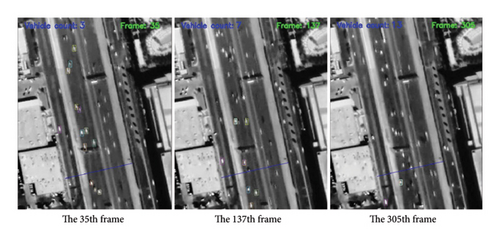
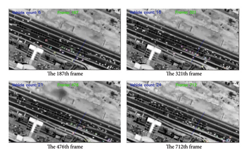
In the traffic flow extraction experiment, the number of cars in the first frame of video unblocked traffic and congested traffic was selected as 13 and 22. Respectively, the virtual detection line only counted the selected vehicles. Figure 11 shows the optimal counting results of vehicle targets under unblocked traffic. In the video, the time for all selected vehicles to pass through the virtual detection line was 6s, and the traffic flow was obtained as 7800 vehicles/h. The traffic flow extraction accuracy of the detection line is 98.48%, indicating the effectiveness of this method in traffic flow extraction under unblocked traffic. Figure 12 shows the count results of vehicle targets in the case of congested traffic. The average count result of the virtual detection line was 24.6 vehicles, the time for all vehicles to pass the detection line was 16s, and the traffic flow is 5400 vehicles/h. In comparison, the traffic flow calculated by the actual value of the vehicle count was 5040 vehicles/h, and the extraction accuracy of the virtual detection line was 90.18%. The virtual detection line is set in the congested driving area. The vehicle’s speed through the virtual detection line is too slow. The virtual detection line will repeatedly count it, resulting in a decrease in the traffic flow extraction accuracy of the detection line, indicating that the vehicle moving speed in the satellite video dramatically influences the accuracy of the virtual detection line.

5. Conclusions

In order to effectively improve the accuracy of traffic flow extraction from satellite video, this paper has proposed a traffic flow extraction method based on improved KCF. First, the improved KCF tracking method was employed to track the vehicle target in the satellite vide. A multifeature fusion method improved the tracker’s ability to distinguish vehicle targets from complex backgrounds, and the Kalman filter predicted the driving trajectory of vehicles during occlusions. Then, through the comparison results with the classical algorithm in the experimental dataset, it can be seen that the tracking precision and success rate of the method in this paper are significantly higher than other classical algorithms, which comprehensively improves the accuracy of vehicle tracking. Finally, based on the tracking results, the virtual detection line was utilized for the traffic flow extraction experiment. The experimental results demonstrated that the traffic flow extraction accuracy of the detection line can reach 98.48%, which proves the feasibility and effectiveness of this method in the case of smooth traffic. However, in the case of traffic congestion, the traffic flow extraction performance of the virtual detection line was reduced, with an accuracy of 90.18%. It is necessary to further study the impact of traffic congestion on traffic flow extraction by virtual detection line. In this paper, traffic flow extraction is studied from a broad perspective, which brings new ideas to the field of traffic information extraction and plays a positive role in promoting the construction of technical infrastructure of ITS.

Conflicts of Interest

The authors declare no conflicts of interest.

Funding

This work was supported by Xinjiang Autonomous Region Key Research and Development Project (2022B01015), Science and Technology Plan Project of Ganquanbao Economic and Technological Development Zone (GKJ2023XTWL04), and Key Laboratory Open Subject (2023ZDSYSKFKT06).