The customized bus in operation faces numerous random factors that affect the service level and attractiveness to passengers. Therefore, this paper investigates the optimization problem of customized bus routes considering random vehicle travel times and the capability to respond to dynamic requests in real time. We developed a stochastic programming model that minimizes total cost and passenger travel time. The innovation lies in the model’s ability to respond to requests made by passengers during service and to model the randomness of vehicle travel times using a known distribution. Furthermore, we propose a heuristic algorithm combining the nondominated sorting genetic algorithm II (NSGA-II) and a variable neighborhood search operator. This algorithm starts by generating an optimized initial path based on initial reservation demands and then employs a dynamic adjustment mechanism to respond to real-time requests. The effectiveness and superiority of our algorithm are validated through an illustrative example. Finally, numerical experiments using taxi trajectory data demonstrate that considering both randomness and real-time aspects can significantly reduce the total cost and penalties for early and late arrivals and improve the bus service level.

1. Introduction

With rapid urban population growth and increasing private vehicle ownership, urban transportation issues such as congestion, air pollution, and noise have become more severe, especially in megacities. These problems mainly stem from the imbalance between growing travel demand and limited transport supply. To address these challenges, reducing dependence on private cars and enhancing public transport services have become key goals of urban transport development. As a demand-responsive service offering flexible, door-to-door transport, customized buses have emerged as an effective solution to ease congestion and pollution [1, 2].

Globally, they are gaining traction, with successful implementations such as Europe’s demand responsive transit (DRT) and the U.S. flexible bus services [3]. In China, the government has actively promoted customized buses, launching over 5400 routes across 29 provinces, serving 180 million passengers annually. In cities such as Beijing, these services cover commuting, corporate shuttles, and tourism needs [4].

Despite their advantages, most customized bus services still rely on fixed routes and timetables, lacking flexibility to adapt to real-time demand fluctuations. Moreover, in practice, vehicles operate on open urban road networks and are affected by random factors such as traffic congestion, accidents, and weather. These uncertainties lead to variability in vehicle travel times and arrival times, which in turn impact both operational costs and service quality, posing significant challenges for route optimization.

Although some studies consider the effect of stochastic arrival times, most focus on conventional fixed-route services. Research on customized buses with flexible routing and real-time demand response is limited, especially in addressing both stochastic travel times and dynamic demand simultaneously.

In summary, this study addresses the problem of dynamic route optimization for customized bus services under stochastic travel times. The main contributions are as follows:

1.
A multiobjective optimization model is proposed that minimizes both the total passenger–operator cost and passenger travel time. The model accounts for real-time passenger requests received during vehicle operation and assumes that vehicle travel times follow a probabilistic distribution, considering the interests of both passengers and operators.
2.
A heuristic algorithm combining nondominated sorting genetic algorithm II (NSGA-II) and variable neighborhood search (VNS) is developed. This approach leverages the global search capability of multiobjective genetic algorithms and the local refinement strength of neighborhood search, leading to improved convergence efficiency.
3.
Numerical experiments are conducted on a benchmark dataset to validate the effectiveness of the proposed model and algorithm. Further evaluation using real-world taxi trajectory data demonstrates that incorporating stochastic travel times can reduce both operator costs and passenger travel time compared to traditional models with deterministic travel times.

The rest of this paper is organized as follows: Section 2 summarizes an overview of the related existing literature. Section 3 constructs a model including both randomness and real-time demand. Section 4 provides the heuristic solution framework in detail. Section 5 presents the numerical experiment and the case study for evaluating the performance of the model and the algorithm. Finally, we conclude this paper and discuss future work in Section 6.

2. Literature Review

The discussion of the literature review covers previous studies in customized bus routing problems with a deterministic and stochastic environment.

2.1. Customized Bus Route Optimization

Accurately identifying passenger demand is critical for optimizing customized bus routes. Currently, most studies rely on methods such as randomly generated travel demand, travel surveys, real-world road network data [5, 6], and public transit smart card data [7, 8] to obtain demand information. However, relatively few studies have explored the use of taxi trajectory data to extract customized bus travel demand and support route optimization [9].

In terms of objective setting, existing studies typically focus on optimizing operator cost, total operational mileage, overall profit, and passenger travel time. Tong et al. [10] constructed a network optimization model to maximize the number of commuters, while He et al. [11] minimized total operating cost under constraints such as routing planning, vehicle capacity, and fleet size. Lyu et al. [12] focused on maximizing operator profits through route planning. Some researchers have considered the interests of both passengers and operators. Guan et al. [13] proposed a biobjective optimization model for customized bus routing that aims to maximize operational profit while minimizing passenger travel cost. Wu et al. [14] incorporated both passenger and operator costs, as well as the number of unserved passengers. Asghari et al. [15] considered carbon emissions, carpooling satisfaction, and vehicle operating costs. Zhou et al. [16] proposed a scheduling model optimizing both operating costs and passenger waiting times. However, most multiobjective approaches adopt a linear weighted sum method, where the choice of weights is often subjective. This makes it difficult to clearly reflect the trade-offs between objectives, potentially leading to solutions that deviate from the true optimum in practice.

In terms of algorithm design, customized bus routing optimization is an extension of the vehicle routing problem (VRP), known to be NP-hard. Some researchers have applied exact methods such as Branch and Bound [17], Branch and Cut [18], and Lagrangian Decomposition [5], while others have combined algorithms to enhance performance. For instance, Huang et al. [19] integrated simulated annealing into a genetic algorithm, reducing parameter selection complexity and expanding the search range. Wang et al. [20] proposed a hybrid genetic-ant colony algorithm (GACA). Xue et al. [21] developed an improved adaptive large neighborhood search (ALNS) method. Ma et al. [22] designed a hybrid encoding strategy based on the NSGA-II with an elitist strategy to optimize customized bus routes. Nevertheless, combining heuristic and multiobjective evolutionary algorithms for customized bus routing optimization remains relatively underexplored. Integrating these two approaches could effectively address multiobjective problems and further improve computational efficiency, highlighting a promising direction for future research.

Moreover, several studies have focused on dynamic adjustment strategies for customized bus services. The dynamic customized bus routing problem typically employs a two-stage optimization approach. An initial route is first generated based on static demand and then dynamically adjusts these routes during real-time operations to accommodate new passenger requests [23–25]. Specifically, Han et al. [26] selected stations with high probabilities of passenger requests based on historical data to construct an initial bus route, adjusting these routes in real-time according to actual demand. To evaluate interactions between passengers and vehicles, Huang [27] proposed a hierarchical decision-making model, first determining passenger acceptance before departure and subsequently optimizing routes for accepted requests using a branch-and-bound algorithm.

2.2. Customized Bus Route Optimization in a Random Environment

In practical customized bus operations, uncertainties such as traffic conditions, passenger fluctuations, and weather significantly impact vehicle travel times, arrival times, and passenger requests. Consequently, optimizing customized bus routes under uncertainty has increasingly attracted scholarly attention, focusing mainly on stochastic demand, travel times, and service times.

Some studies apply robust optimization methods to handle uncertainties in travel demand and operational environments. For example, Dou et al. [28] considered uncertainty in passenger demand and developed a robust optimization model for customized bus systems with different vehicle types. Jiao et al. [29] addressed uncertain travel times in electric bus systems between urban and rural areas through a robust optimization model.

Additionally, some scholars assume that random variables follow specific probability distributions and employ stochastic programming methods. Chen et al. [30] optimized regular bus routes considering normally-distributed vehicle arrival times, demonstrating that neglecting these stochastic arrival times reduces service quality. Fachini et al. [31] proposed a two-stage stochastic mixed-integer programming model incorporating random travel times, finding that accounting for random travel times yielded more feasible solutions.

Meanwhile, other researchers considered time-dependent travel times. Guo et al. [32] developed a time-dependent customized bus routing optimization model incorporating traffic congestion and alternative routes, illustrating that operating costs rise with increasing congestion levels. Wang et al. [33] addressed time-dependent energy due to time-varying vehicle speeds and developed a routing optimization method with time windows and multiple depots, enhancing planning flexibility and efficiency.

Despite significant progress addressing uncertainties in public transit systems, most existing research primarily focuses on traditional fixed-route transit. Thus, there remains insufficient exploration of dynamic customized bus routing optimization under uncertainty.

3. Model Formulation

3.1. Problem Statement

Figure 1 shows the problem studied in this paper. Considering the stochasticity of vehicle travel times, this research aims to reasonably plan the initial operational routes for customized buses according to passengers’ travel demands, which include origin (o_p), departure time (t^o(p)), destination (d_p), and arrival time (t^d(p)). While the vehicles operate these initial requests according to the predetermined routes, the system collects newly received real-time travel requests at intervals of time t and dynamically adjusts the initial routes based on this real-time passenger information. The objective is to minimize passenger travel times and operator costs simultaneously, thus effectively balancing benefits for both passengers and operators.

Details are in the caption following the image — **Figure 1**
Open in figure viewer PowerPoint

Diagram of the customized bus routing optimization problem.

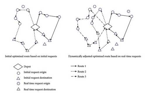
The customized bus route optimization can be defined by a graph G = (V, A), where V is the set of all nodes. The node set V = {0, 1, 2, …, 2n, 2n + 1} consist of depots {0, 2n + 1} and stations N = {1, …, 2n}. Nodes 0 and 2n + 1 represent the same depot, meaning each vehicle departs from depot 0 and returns to depot 2n + 1. N consists of a set of pick-up stations denoted as N⁺ and a set of drop-off stations denoted as N⁻. Each pair of node (i, n + i) is associated with the o_p and d_p of passenger p.

A is a set of arcs, A = {(i, j) : i ∈ V, j ∈ V, i ≠ j}, that connects each pair of nodes. Each arc (i, j) is associated with a travel distance len(i, j) and a travel time t(i, j), where len(i, j) is symmetrical, i.e., len(i, j) = len(j, i). Considering the dynamic effects of actual road conditions, the travel time t(i, j) is modeled as a normally distributed random variable [34]. Moreover, travel times on different arcs are assumed to be independent, i.e., , where μ_ij and represent the mean and standard deviation of the travel time, respectively.

To simplify the problem, we make the following hypothetical assumptions:

1.
Passenger travel demands are known. If a demand falls within the service range of a specific route, the corresponding passenger will choose that route for travel.
2.
The service area is divided into origin and destination areas. Stops in the origin area serve only boarding passengers, while stops in the destination area serve only alighting passengers.
3.
Depots are treated as virtual nodes. To simplify the model, the travel cost between the departure depot and the first boarding stop, as well as between the last alighting stop and the arrival depot, is assumed to be zero.
4.
Only one type of vehicle is used for customized buses, meaning all vehicles have the same maximum passenger capacity.
5.
Vehicle travel times follow a known probability distribution.

3.2. Model Construction

3.2.1. Initial Optimization Phase

Both passengers and operators have distinct objectives to optimize. Passengers hope to minimize their travel time and costs, while operators seek to reduce the operational costs of bus routes. To balance these conflicting objectives, our model is formulated as a multiobjective optimization problem, simultaneously minimizing the total costs and passenger travel time. By considering both perspectives, the model ensures an optimal trade-off between efficiency and service quality.

For the convenience of the reader, we provide Table 1 listing the notation used in the model during the initial optimization phase.

Table 1. Notation definitions.

Notation		Definition
Set	V	Set of customized bus stations
	A	Set of links
	K	Set of initial vehicles
	P	Set of initial passenger requests

Parameter	f1	Ticket price per kilometer
	f2	Operational cost per kilometer of a vehicle
	Q(k)	Number of seats in the vehicle k
	α_k	Lowest load factor of the vehicle k
	v	Average speed of private cars
	t_p(i, j)	Travel time of the passenger p from the stop i to j
	len(i, j)	Travel distance from the stop i to j
		Time window of the vehicle k to the stop i that the passenger p can endure
	(o_p, d_p)	Origin and destination of the passenger p
	ω	Weight factor balance between losing a candidate passenger and operating cost
	s(i)	Service time for boarding and alighting at the station i
	λ₁, λ₂	Penalty factor of early and late arrival
	E[·]	The expected value of a random variable

Variable		If the passenger p is transported by the vehicle k, ;otherwise,
		If arc (i, j) is selected by the vehicle k, ;otherwise,
		Arrival time of the vehicle k at the stop i

3.2.1.1. Objective Function

()

Equation (1) indicates that the total of the operating costs and passenger ticket costs is minimized. A larger ω implies that the operator prioritizes minimizing operational costs, possibly at the expense of passenger service quality. Conversely, a smaller ω indicates that the operator is willing to bear higher costs to provide better service and retain more passengers. Equation (2) represents the minimization of passengers’ travel time, which consists of two components. The first component is the difference between the actual travel time on the customized bus and the “shortest-path time.” Here, the “shortest path” refers to the travel time under a direct taxi service, i.e., the minimum time required to travel directly between two stops. The second component is the penalty for violating the time windows at stops, including penalties for both early arrivals (arriving before the lower bound of the time window) and late arrivals (arriving after the upper bound).

3.2.1.2. Constraints

Allocation constraints: Each passenger can only be served by a customized bus.

()

Vehicle capacity constraints: To ensure the “one-person-one-seat” service level, the total number of served passengers cannot exceed the capacity of the vehicle.

()

Operator profitability constraints: To guarantee the operator’s profitability, each bus line must reach minimum capacity.

()

Service area constraints: Each vehicle departs from the depot and must return to it upon completing its route. And the vehicle is required to first serve the boarding area and then the alighting area.

()

Flow balance constraints: To make sure that each vehicle k can find a feasible route,

should satisfy the flow balance constraint.

()

Binary constraints: Impose the binary constraints for the variables

and

()

3.2.2. Dynamic Adjustment Phase

The main difference between the dynamic adjustment phase and the initial optimization phase lies in the demand points. In the initial phase, demand points include only prebooked requests P. In the dynamic stage, demand points consist of two parts at time t, real-time requests P_t that have already been received, and unvisited requests P_t,2. Table 2 lists the notation used to the dynamic phase modeling.

Table 2. Notation for the dynamic adjustment phase.

Notation		Definition
Set	P_t	Set of real-time passenger requests at time t
	P_t,1	Set of visited passenger requests at time t
	P_t,2	Set of unvisited passenger requests at time t
	K_t	Set of newly dispatched vehicles for real-time demands at time t
	K_t,1	Set of dispatched vehicles that have returned to the depot at time t
	K_t,2	Set of dispatched vehicles that have not yet returned to the depot at time t

Parameter	Q_t(k)	Remaining capacity of the vehicle k at time t, for newly dispatched vehicles, Q_n(k) = Q(k)

Variable		If the passenger p is transported by the vehicle k, ; otherwise,
Variable		If arc (i, j) is selected by the vehicle k, ; otherwise,

The objective function can then be stated as expression (12) and (13), subject to constraints (14)–(22).

()

Equations (12) and (13) define the objective functions for dynamic route adjustment based on real-time demand statistics at time t, where equation (12) represents the passenger-operator cost and equation (13) represents the passenger travel time. The constraints for the dynamic adjustment phase are given in equations (14)–(22), with their interpretations provided in equations (3)–(11).

3.2.3. Analysis of the Objective Function

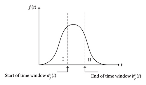
The objective function of the modified stochastic programming model proposed in this paper consists of three components. The latter two parts represent penalties for vehicle arrivals at stations earlier or later than their time windows, respectively. The expected values of early arrival and late arrival at the stop i for the vehicle k can be calculated using the probability density function of vehicle arrival times [30].

Assuming that the travel time follows a normal distribution, the arrival time is also normally distributed. Figure 2 shows a probability density. In Area I, the bus arrives early; in Area II, the bus arrives late.

The probability density function and distribution function of vehicle arrival time are as follows:

()

The expected value

of the vehicle’s early arrival time at the station can be calculated using the following process:

()

Similarly, the expected value

of the vehicle’s delayed arrival time at the station is as follows:

()

where

denotes the expectation of the passenger p for the arrival time of the vehicle k at the station i;

denotes the standard deviation of the passenger p for the time of the vehicle k arriving at the station i; and Φ(x) denotes the standard normal distribution function.

4. Solution Algorithm

The NSGA-II is commonly used for the multiobjective optimization problem but often struggles with search ability and convergence. Therefore, we propose a heuristic approach based on the NSGA-II algorithm.

We introduced a greedy strategy for population initialization and an evolutionary strategy using a VNS operator to enhance convergence speed. The initial route is optimized based on reservation requests, and real-time requests are dynamically adjusted using a local search based on the insertion method.

4.1. Initial Route Optimization Phase

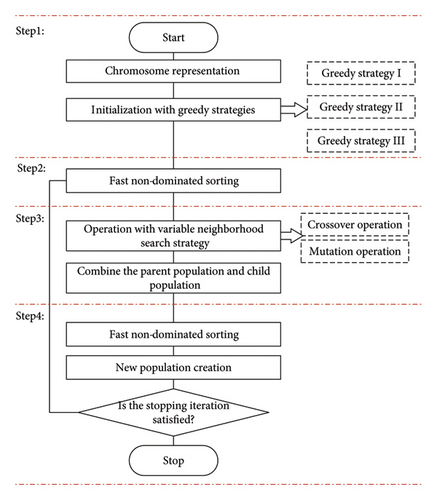
In the initial optimization phase, we propose an improved NSGA-II algorithm, which addresses the problem through four steps, as shown in Figure 3.

4.1.1. Chromosome Encoding

In this paper, the chromosome is encoded by a two-stage coding method. The first segment of the chromosome consists of the number of each boarding station, and the length is the total number of boarding stops. The second segment of the chromosome consists of the number of each bus alighting station, and the length of the chromosome is the total number of alighting stops.

Suppose that a road network contains a customized bus depot (numbered 0). Five passengers have boarding stations numbered one to five and corresponding alighting stations numbered 6–10. A two-stage chromosome is randomly generated as 1-4-5-2-3-9-6-7-10-8, which decodes into three vehicle routes, 0-1-4-9-6-0, 0-5-2-7-10-0 and 0-3-8-0.

4.1.2. Population Initialization With Greedy Strategies

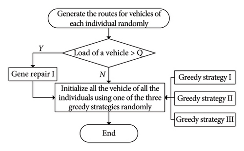
The initial population was constructed using a greedy strategy and a random method. Figure 4 presents the flowchart of the initialization. If the vehicle violates the maximum passenger capacity constraint, gene repair strategy I is adopted by randomly removing or swapping a stop with another route until the constraint is satisfied. Subsequently, one of the three greedy strategies is used to initialize the vehicle path randomly. Greedy strategy I prioritizes serving passengers closest to the bus depot; greedy strategy II serves the site with the highest demand first; and greedy Strategy III prioritizes passengers with the earliest departure time. Therefore, greedy strategies I and II increase the operator profit, while strategy III reduces passengers’ travel costs.

4.1.3. Operation With the VNS Strategy

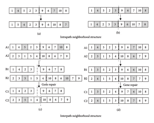
We integrate the VNS operator into the crossover and mutation operations in the NSGA-II to change the order of vehicles serving passengers and find better solutions. Four neighborhood operators were designed for a VNS between and within routes, as shown in Figure 5.

Since we employ a two-stage chromosome encoding scheme, crossover and mutation operators are applied separately to each segment. The detailed description is as follows:

In the intrapath neighborhood structure, we assume five boarding stations (numbered 1–5) and five corresponding alighting stations (numbered 6–10), and a chromosome is randomly generated as 1-4-5-2-3-9-6-7-10-8.

1.
Relocation. Within each segment (boarding and alighting stations), randomly select one gene, remove it, and then reinsert that gene at another randomly chosen position within the same segment, as shown in Figure 5(a).
2.
2-Opt. Within each segment, randomly choose two distinct gene positions, reverse the subsequence between these positions, and reconnect the segment ends, as shown in Figure 5(b).

In the interpath neighborhood structure, two chromosomes are randomly generated as A1: 1-4-5-2-3-9-6-7-10-8 and A2: 2-3-1-5-4-10-8-6-7-9.

1.
Insert: For each chromosome, randomly select one gene from its boarding segment and one from its alighting segment and then insert each into a random position in the corresponding segment of the other chromosome. If a duplicate gene results, delete its second occurrence to restore feasibility, as shown in Figure 5(c).
2.
Swap: For each chromosome pair, randomly pick one gene from the boarding segment of each chromosome, swap these two genes, and repeat the same process for the alighting segments. If this exchange produces duplicates outside the swapped positions, resolve them by exchanging the redundant nodes according to the original gene-mapping relationship established within the matched region, as shown in Figure 5(d).

The interpath neighborhood structure is used to select stations from two lines randomly for exchange operations. The intrapath neighborhood structure is used to select stations from the line for operation. The pseudo code of the crossover operation is given in Algorithm 1.

Algorithm 1: Crossover operation

Input: Parent population Pop
Crossover operators (Relocation, 2-Opt, Insert, Swap)
Crossover probability P_c
Output: Child population Pop^′
1.
Fori = 1 : 4
2.
Select an operator from the four crossover operators randomly (Relocation, 2-Opt, Insert, Swap)
3.
Select the optimal individual with non-dominated sorting
4.
Implement crossover operation, and generate offspring individuals
5.
If The new individual is better than the current optimal individual
6.
This operator is used as a contemporary crossover operator to generate new individuals
7.
Break
8.
Else
9.
Select an operator from the four crossover operators randomly to implement crossover operation (Relocation, 2-Opt, Insert, Swap)
10.
End If One of the four operators is randomly selected as the crossover operator
11.
End For
12.
End

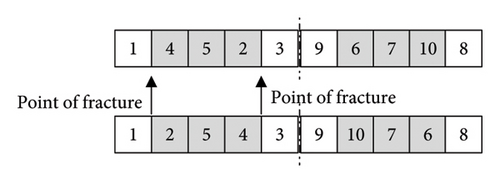
To improve the algorithm’s individual and local search capabilities, we introduce a reversal operator, where the chromosome is split at two random points and the segment is reversed, as shown in Figure 6. The pseudo code for the mutation operation is shown in Algorithm 2.

Algorithm 2: Mutation operation

Input: Parent population Pop
Mutation operators (Insert, Reverse)
Mutation probability P_m
Output: New individual Pop_i
1.
IfP_m ≥ random[0, 1]
2.
Select a parent individual randomly
3.
Select an operator from the two mutation operators randomly (Insert, Reverse)
4.
Implement mutation operation, and generate offspring individuals
5.
End If
6.
End

4.1.4. Fast Nondominated Sorting and Elitism Preservation Strategy

We used fast nondominated sorting and elitism preservation strategies to ensure the diversity and quality of solutions. Fast nondominated sorting ranks the population, assigning a rank and crowding distance to each individual. The rank is based on the number of individuals dominated by the individual i and the number of individuals that can dominate the individual i, while the crowding distance is the distance between the objective functions of the two individuals neighboring a specified individual.

All individuals, including parents and offspring produced through crossover and mutation, are mixed to create a new population. This new population is then subjected to nondominated sorting for graded selection, forming a new population with different levels of noninferior solutions. If the noninferior solution front Z1 meets the population size requirements, the sorting by crowding distance is stopped. If Z1 does not fulfill the requirements, individuals from Z2 with larger crowding distances are selected until the population size is satisfied [35].

4.2. The Dynamic Optimization Phase

When a passenger has a dynamic request, the operator must decide whether to respond. In the initial stage, the bus route was planned based on the reservation request. During the dynamic adjustment phase, the route is updated in real time to accommodate new requests. Referring to the proposed heuristic algorithm [12, 27] and considering interactive decision-making between passengers and operators, this study proposes a dynamic optimization adjustment method based on local search with the following specific steps:

Step 1. Initialization parameter.
Input:
- 1.
  The route J_k generated in the initial optimization stage includes the actual arrival time and actual departure time of each vehicle.
- 2.
  Newly received passenger p requests for information [o_p, t^o(p), d_p, t^d(p)]
- 3.
  Time to start responding to the dynamic request t
- 4.
  Number of vehicles k;
Step 2. Determine the vehicle status.
- 2.1. Determine which nodes each vehicle k has served and which nodes have not been served at time t;
- 2.2. Determine whether there is a demand point that the vehicle k is not serving. If it exists, the first unserved demand point for the vehicle k is taken as the starting point of the vehicle in the dynamic phase, and the actual departure time from the first unserved point and the remaining capacity of the vehicle are calculated.
Step 3. Dynamic optimization adjustment.
- 3.1. Select the vehicle k that does not have a service demand point to continue to complete the subsequent service.
- 3.2. Remove the station that has not been served at time t from the route J_k, and only retain the path of the service node at time t;
- 3.3. The deleted requirement points and real-time requests are merged into a new set of unserved requirement points
- 3.4. The initial population of the dynamic optimization adjustment phase is randomly generated, and the unserved demand is randomly assigned to each vehicle without violating the vehicle capacity limit. If the dispatched vehicle cannot serve all the demand points, a new vehicle is dispatched, and the corresponding demand points are assigned.
- 3.5. The improved NSGA-II is used for optimization
Step 4. Produce the optimal vehicle route after dynamic optimization adjustment.

5. Experiment

This section implements a standard data test of the proposed model and algorithm and then uses a real taxi trajectory dataset to study the route planning for the study area.

5.1. Benchmark Results

We used the standard data test of the bus route problem provided by Park et al. [36], which is a similar situation to the customized bus network. The original benchmark instances are available in the following URL: https://logistics.postech.ac.kr/Mixed_SBRP_Benchmark.html.These examples were modified to adapt to the problems in this study. We selected ten examples from a standard dataset to verify the effectiveness of the improved NSGA-II. R and C represent random and dense distributions of stations, respectively, and n represents the number of stations. The ticket price per kilometer and operational cost per kilometer were held constant, but the passenger demand distribution varied.

5.1.1. Pareto Solutions

The proposed heuristic algorithm was tested on a personal laptop (Intel Core i7, 8G, 2.0 GHz) through MATLAB R2019a, and each example was run 10 times. The parameters used in the model and algorithm are listed in Table 3.

Table 3. Algorithm and model parameters.

Algorithm parameter	Value	Model parameter	Value
Popsize	100	Q(k)	30
Maxiteration	500	α(k)	50%
p_c	0.9	f1	3 $/km
p_m	0.1	f2	9 $/km
		v	45 km/h

The Pareto solutions generated by the proposed and original NSGA-II algorithms for the four examples are presented in Figure 7. Each point in the graph represents a customized bus route plan. The graph shows that the nondominated solutions we obtained were closer to the Pareto-optimal frontier than the original NSGA-II, indicating that the proposed algorithm outperformed the original NSGA-II. The Pareto frontier distribution was relatively uniform, and the population diversity was good.

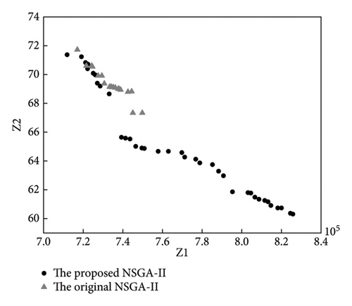
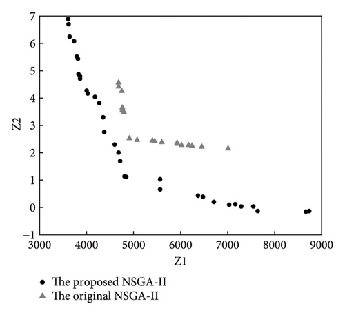
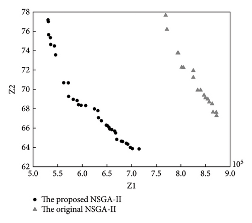
To compare the performance of the two algorithms, we used metrics from Rabiee et al. [37], diversity DM, average ideal distance MID, and a quality index QM. Among them, DM determines the diversity of nondominated solutions obtained by the algorithm, with higher values indicating better performance. MID represents the average distance between the Pareto solution and the ideal point, and it is inversely proportional to the algorithm performance. QM is the percentage of the original solution in the new nondominated solution set; the larger its value, the better the performance of the algorithm. The experimental comparison results are shown in Table 4.

Table 4. Comparative analysis of the algorithm.

Instance ID	n	DM		MID		QM
Instance ID	n	Improved NSGA-II	NSGA-II	Improved NSGA-II	NSGA-II	Improved NSGA-II	NSGA-II
R1	20	3934.88	2331.55	5200.19	5467.32	64.71	35.29
C2	50	184,792.1	155,464.5	617,839.4	842,831.3	57.14	42.86
C3	50	113,651.1	41,309.5	728,498.5	766,076	64.91	35.09
R4	50	224,693.6	28,101.35	2,034,559	3,753,721	82.61	17.39
C5	80	162,470.5	97,597.2	4,931,336	9,867,566	73.33	26.67
R6	80	1,255,931	130,439.1	4,874,166	7,845,604	84.00	16.00
R7	100	199,135.9	58,006.1	4,314,059	5,680,894	76.9	23.1
C8	100	257,343.9	52,802.03	4,245,963	7,025,822	80.00	20.00
R9	100	1,192,649	120,169.2	6,586,447	8,303,946.3	70.13	29.87
C10	100	63,264.7	56,791.1	7,671,628	14,583,646	85.00	15.00

The improved NSGA-II demonstrated faster convergence and better local search capabilities compared to the original. As shown in Table 4, the improved NSGA-II obtained a smaller MID, which indicates a more evenly distributed Pareto solution set. It also produced a higher DM, reflecting a broader search across solution spaces. Overall, the Pareto solution set from the improved NSGA-II had clear advantages.

5.1.2. Dynamic Optimization Adjustment Analysis

To verify the proposed dynamic optimization method, an R1 example was selected. Ten passenger reservation requests were randomly generated at t. The improved NSGA-II and dynamic adjustment strategy were used to update the route in real time. The solution with the lowest passenger travel cost in the Pareto solution set was selected for analysis. The final scheme is presented in Table 5.

Table 5. Comparison of two scenarios.

Vehicle number	Initial optimization route	Dynamic optimization route
1	0-1-(2)-(3)-4-(5)-6-7-0	0-1-(2)-(3)-4-(5)-6-7-0
2	0-8-14-13-9-(10)-(11)-0	0-8-14-13-23-0
3	0-12-17-(18)-(19)-15-(16)-0	0-12-17-(18)-(19)-22-(21)-(20)-0
4		0-25-15-(16)-9-(10)-(11)-0

Note: Numbers in parentheses represent sites with different numbers but the same geographical location.

In Table 5, since all the stations of vehicle 1 were served at time t, the path plan was not changed. Vehicle 2 and vehicle 3 responded to the dynamic requests of some passengers at t, resulting in midway route changes. Some passengers’ needs could not be inserted into the existing routes. To address unserved passenger requests and unanswered passenger requests, the operator assigned vehicle 4 a route. The initial optimization scheme and the dynamic optimization scheme in Example R1 are shown in Figures 8 and 9, respectively. Geographic coordinates (latitude and longitude) have been converted into a planar coordinate system for clearer visualization and analysis.

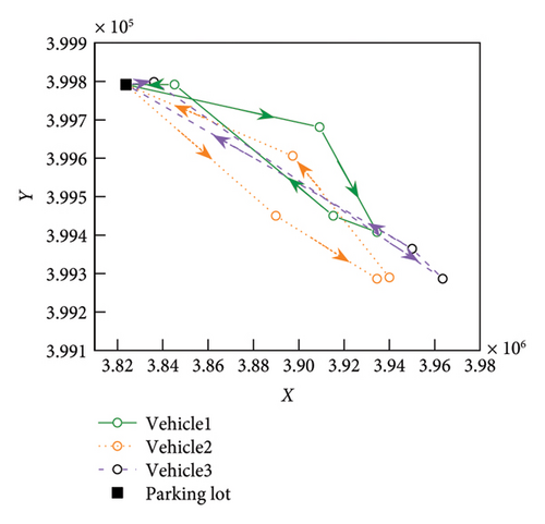
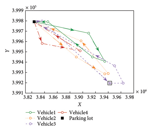
The results show that the improved NSGA-II algorithm not only planned a reasonable initial route based on the initial request but also updated the route for real-time requests, meeting the needs of most passengers. In other words, the proposed algorithm and the update mechanism can solve the dynamic route optimization problem for customized bus services.

5.1.3. Random Variable Analysis

We assume that the travel time of a vehicle is a normally distributed random variable. To test the addition of random variables to the objective function, we set the variance of the vehicle travel time to 0.1, 0.2, 0.3, and 0.4 of the mean value. Repeating each group of variance levels ten times, we selected the solutions with minimum passenger travel cost in the Pareto set and analyzed the influence of the addition of random variables. The results are presented in Figure 10.

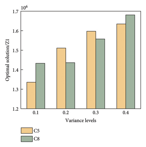
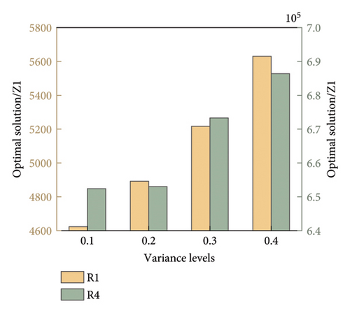
Figure 10 shows that increasing the variance level increased the randomness of the vehicle travel time, leading to suboptimal results. In most examples, setting the variance at 0.1 produced significantly better results than at 0.2, 0.3, or 0.4. Therefore, we set the variance to 0.1 for all subsequent experiments.

5.2. Case Study

Taxi trajectory data are reliable sources for estimating travel demand for customized bus services, as it provides comprehensive and detailed information about passenger travel and reveals the actual demand throughout a city. Some taxi passengers choose this mode of transport due to their preference for direct, fast, and comfortable travel. However, customized buses can offer similar service quality with the added advantage of lower fares, making these passengers potential users. Therefore, this study utilizes a taxi trajectory dataset to design customized bus routes that meet urban travel demand efficiently and affordably.

We used GPS data from 4316 taxis in Shanghai, China, on a given day; the average frequency of GPS records is about 32 s. The records relevant to our study include taxi ID, timestamp, latitude and longitude, and the vehicle’s occupancy status. By detecting passengers’ boarding and alighting activities, we extract passengers’ travel trajectories. Then, each taxi passenger’s trajectory was considered as a travel demand, meaning the boarding and alighting locations and times in the taxi trajectory data serve as the origin, destination, and departure time for the customized bus passenger demand. Based on the method described in the paper of Lyu et al. [12], we selected 24 customized bus stations, where there are twelve boarding stops (numbered 1-12) and twelve alighting stops (numbered 13–24). The parameters used in the model and algorithm are the same as those in Table 2.

5.2.1. Result Analysis

We used the improved NSGA-II algorithm to solve stochastic and deterministic models of customized bus routes. The iterative process of the algorithm is illustrated in Figure 11.

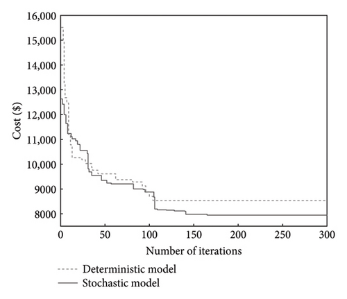
Figure 11 shows that adding random variables increased the model’s complexity, resulting in more iterations. The lowest cost was achieved when the number of iterations reached around 175. As seen in Figure 12, the Pareto-optimal solution set shows that the stochastic model had a lower total system and passenger travel time costs compared to the deterministic model. Therefore, considering random factors not only reduced total system costs but also improved passenger travel efficiency.

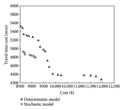
Using the results of several operations, we selected the best route optimization scheme. We compared the Pareto solutions with the lowest passenger travel time cost and the lowest total cost (Schemes 1 and 2 in Table 6). Table 6 lists the optimal bus routes and the average passenger travel times under the stochastic and deterministic models, respectively.

Table 6. Optimal routing and average passenger travel times.

Scenarios	Scheme	Vehicle ID	Vehicle route	Number of passengers	Average travel time of passengers (min/pass)
Deterministic model	1	1	0-11-4-1-2-8-41-35-34-37-44-0	30	62.1
		2	0-10-6-3-9-42-39-43-36-0	23	54.3
		3	0-5-7-12-40-38-45-0	15	55.2
	2	1	0-11-2-44-35-0	18	35.2
		2	0-4-12-6-1-8-10-37-41-39-43-45-34-0	22	56.8
		3	0-5-7-3-9-42-38-40-36-0	28	60.5

Stochastic model	1	1	0-9-12-45-42-0	16	38.2
		2	0-6-8-11-10-43-39-44-41-0	19	46.9
		3	0-4-1-7-5-37-34-38-40-0	18	49.2
		4	0-2-3-35-36-0	15	36.1
	2	1	0-7-2-40-35-0	15	25.4
		2	0-12-5-1-34-38-45-0	15	37.8
		3	0-10-4-3-8-41-37-36-43-0	15	43.5
		4	0-9-6-11-44-39-42-0	23	50.3

Note: 34∼45 represent station number 13∼24, respectively.

According to the deterministic model in Table 6, the average full load rates for Schemes 1 and 2 exceeded 75%, indicating better bus resource utilization from the operator’s perspective. However, from the passengers’ perspective, the average travel time in Scheme 1 was 12.6% higher than in Scheme 2. In the stochastic model, most vehicle load rates in both schemes were approximately 60%. While both schemes showed similarly good load rates, the average passenger travel time was slightly lower in Scheme 2. We used Scheme 2 with better passenger travel time to compare the stochastic and deterministic models, repeating each experiment group ten times. The results are shown in Table 7.

Table 7. Results for the deterministic and stochastic models.

Results	Deterministic model	Stochastic model
Passenger travel time cost (min)	5509.1	5094.3
Total cost ($)	10,158.7	9530.6
Operator cost ($)	5030.9	5462.3
Early and late arrival penalties (min)	3685.6	1877.6
Average travel time of passengers (min/pass)	61.8	42.6
Number of vehicles	3	4

Table 7 shows that the stochastic model reduced early/late arrival penalties by 49.1% compared to the deterministic model. It also lowered the total cost for passengers and operators by 6.2% and reduced passenger travel time by 7.5%. However, the stochastic models required one additional vehicle, increasing costs by 8.6%. In summary, modeling random variation in vehicle travel times is more in line with reality, reduces early/late arrival penalties, and enhances passenger travel efficiency, ultimately improving the service of customized buses.

5.2.2. Dynamic Optimization Results

The dynamic optimization adjustment phase responds to passengers’ real-time requests by updating the route in real time. We tested the dynamic requests generated after the vehicle had been running for 5 min. We assumed that after the operator processes the real-time request provided by the passenger, six new boarding stations and six new drop-off stations were added.

Table 8 shows the optimal Pareto solution set after the dynamic optimization adjustment. Pareto solution 1 minimizes total cost, while Pareto solution 2 minimizes passenger travel time cost.

Table 8. Dynamic optimization adjustment results.

Vehicle ID	Initial optimization route	Number of passengers	Pareto solution	Vehicle ID	Dynamic adjustment route
1	0-9-12-45-42-0	16	1	1	0-9-12-18-3-42-45-51-36-0
1	0-9-12-45-42-0	16		2	0-6-8-11-10-17-16-49-44-41-43-50-39-0
2	0-6-8-11-10-43-39-44-41-0	19		3	0-4-1-13-7-15-46-40-37-34-48-0
2	0-6-8-11-10-43-39-44-41-0	19		4	0-2-14-5-38-35-47-0

3	0-4-1-7-5-37-34-38-40-0	18	2	1	0-9-12-11-10-43-42-45-44-0
3	0-4-1-7-5-37-34-38-40-0	18		2	0-6-8-17-18-16-5-14-51-38-50-41-40-39-35-0
4	0-2-3-35-36-0	15		3	0-4-1-13-7-15-46-40-48-37-34-0
4	0-2-3-35-36-0	15		4	0-2-3-35-36-0

Table 8 shows that dynamically responding to passenger needs did not increase the number of vehicles used. In both solutions, while the passenger load rate of some vehicles fell below 70%, most vehicles had a load rate above 80%, indicating better resource utilization compared to the initial scheme. Figure 13 compares the vehicle load rates across different schemes.

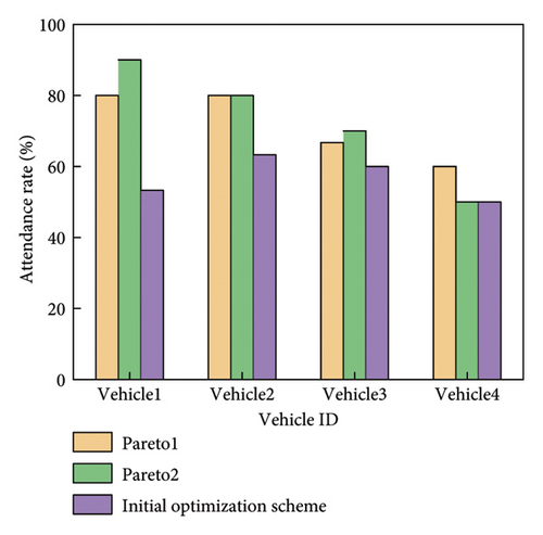
We compared the proposed dynamic optimization adjustment scheme with two alternatives: adding vehicles to serve real-time requests and rejecting real-time requests. The results are shown in Table 9.

Table 9. Comparison results of different optimization scenarios.

Scenario	Operator cost ($)	Number of rejections	Number of vehicles	Average attendance rate (%)	Average travel time of passengers (min/pass)
Dynamic optimization adjustment	6650.9	0	4	70	47.9
Increase vehicles	7520.3	0	5	55.3	44.1
Reject the request	5462.3	7	4	56.7	42.6

As shown in Table 9, rejecting passenger requests directly reduces operator costs, as the penalty for doing so is not considered. However, it also leads to a loss of passenger flow, lowering satisfaction and operational quality. Rearranging vehicles for real-time requests raises costs and lowers load rates, resulting in underutilization of resources. In contrast, the dynamic optimization adjustment scheme reduces operator costs and improves vehicle load rates. Although average passenger travel time increases slightly, it remains within acceptable limits. Overall, the proposed method offers timely responses and reduces operating costs.

6. Conclusions

We proposed a customized bus route optimization model that accounts for random travel times and real-time responses to dynamic demand, aiming to minimize passenger travel time and total costs for both passengers and operators. Based on a stochastic model, we used an improved NSGA-II to solve this problem.

The improved NSGA-II algorithm showed higher computational efficiency due to adaptive, greedy, and evolutionary strategies combined with a VNS operator. It has strong local search abilities and can obtain a more evenly distributed Pareto solution set.

Our case study demonstrated that the travel plan obtained by considering random travel times more accurately captures reality. This reduces the total cost and early/late arrival penalties and improves passenger travel efficiency, thus promoting the operational quality of the customized bus. The dynamic optimization and adjustment strategy provides immediate responses to dynamic passenger requests, reducing operational costs without compromising passenger satisfaction and improving overall service quality.

Future studies should focus on three issues. First is exploring different probability distributions, such as lognormal and gamma distributions. Second, the cost-sharing mechanisms that allow operators to reject infeasible or unprofitable requests implicitly should be considered. The final one is developing more efficient algorithms to balance quality and efficiency in large-scale dynamic scenarios.

Conflicts of Interest

The authors declare no conflicts of interest.

Author Contributions

The authors confirm contribution to the paper as follows. Study conception and design: Fangyuan Gong; data collection and processing: Chuanjun Jia; analysis and interpretation of results: Fangyuan Gong and Xu Wu; draft manuscript preparation: Fangyuan Gong. All authors reviewed the results and approved the final version of the manuscript.

Funding

This research did not receive any specific grant from funding agencies in the public, commercial, or not-for-profit sectors.

Open Research

Data Availability Statement

The data that support the findings of this study are available from the corresponding author upon reasonable request.

References

1 Liu T. and Ceder A., Analysis of a New Public-Transport-Service Concept: Customized Bus in China, Transport Policy. (2015) 39, 63–76.
10.1016/j.tranpol.2015.02.004
Web of Science® Google Scholar
2 Shuai F., Requirement and Prospect of Sustainable Transport for Public Transport: Speech by Lu Huapu Director of Institute of Transport, Tsinghua University, 1, 2021 China (Beijing) International Public Transport Conference, 2022, People’s Public Transport, 54–59.
Google Scholar
3 Zhao Y., Feng Z., and Li X., Transfer-Based Customized Bus Network Design with Holding Control and Heterogeneous Fleet, IEEE Transactions on Evolutionary Computation. (2024) .
10.1109/TEVC.2024.3498315
Google Scholar
4 Liu T., You H., Gkiotsalitis K., and Cats O., Human-Machine Collaborative Decision-Making Approach to Scheduling Customized Buses with Flexible Departure Times, Transportation Research Part A. (2024) 187.
Google Scholar
5 Guo H., Wang Y., Shang P., Yan X., and Guan Y., Customized Bus Route Design with Passenger-To-Station Assignment Optimization, Transportmetrica: Transportation Science. (2024) 20, no. 3.
Google Scholar
6 Chen X., Wang Y., Wang Y., Qu X., and Ma X., Customized Bus Route Design with Pickup and Delivery and Time Windows: Model, Case Study and Comparative Analysis, Expert Systems with Applications. (2020) 168.
Google Scholar
7 Shen C., Sun Y., Bai Z., and Cui H., Real-Time Customized Bus Routes Design with Optimal Passenger and Vehicle Matching Based on Column Generation Algorithm, Physica A: Statistical Mechanics and Its Applications. (2021) 571.
10.1016/j.physa.2021.125836
Web of Science® Google Scholar
8 Zhang B., Zhong Z., Sang Z., Zhang M., and Xue Y., Two-level Planning of Customized Bus Routes Based on Uncertainty Theory, Sustainability (Basel). (2021) 13, no. 20.
Web of Science® Google Scholar
9 Lyu Y., Chow C. Y., Lee V. C., Li Y., and Zeng J., T2CBS: Mining Taxi Trajectories for Customized Bus Systems, IEEE Conference on Computer Communications Workshops, 2016, IEEE, 441–446.
Google Scholar
10 Tong L. C., Zhou L., Liu J., and Zhou X., Customized Bus Service Design for Jointly Optimizing Passenger-To-Vehicle Assignment and Vehicle Routing, Transportation Research Part C: Emerging Technologies. (2017) 85, 451–475.
10.1016/j.trc.2017.09.022
Web of Science® Google Scholar
11 He D., Guan W., Liu T., and Zhang W., Coordinated Operation of Fixed-Route and Demand-Responsive Feeder Transit Services in a Travel Corridor, Journal of Transportation Engineering, Part A: Systems. (2023) 149, no. 2.
10.1061/JTEPBS.TEENG-7505
PubMed Web of Science® Google Scholar
12 Lyu Y., Chow C. Y., Lee V. C., Ng J. K., Li Y., and Zeng J., CB-planner: A Bus Line Planning Framework for Customized Bus Systems, Transportation Research Part C. (2019) 101, 233–253.
10.1016/j.trc.2019.02.006
Web of Science® Google Scholar
13 Guan Y., Wang Y., Guo H., Liu X., and Yan X., Optimizing Customized Bus Services for Multi-Trip Urban Passengers: A Bi-objective Approach, IET Intelligent Transport Systems. (2024) 18, no. 11, 2224–2241.
10.1049/itr2.12569
Web of Science® Google Scholar
14 Wu Y., Yuan Z., Xiao Q., and Yang D., Customized Bus Scheme Design of Large Transport Terminals with Jointly Optimization of Departure Time, Vehicle Allocation and Routing, IET Intelligent Transport Systems. (2022) 17, 85–101.
10.1049/itr2.12240
Web of Science® Google Scholar
15 Asghari M., Al-E S. S. M. J. M., and Rekik Y., Environmental and Social Implications of Incorporating Carpooling Service on a Customized Bus System, Computers & Operations Research. (2022) 142.
10.1016/j.cor.2022.105724
Web of Science® Google Scholar
16 Zhou X., Xi J., Guan Z., and Ji X., Dispatching Design for Customized Bus of Hybrid Vehicles Based on Reservation Data, Journal of Advanced Transportation. (2021) 1.
Google Scholar
17 He X., Yang Z., Fan T., Gao J., Zhen L., and Lyu J., Branch and Price Algorithm for Route Optimization on Customized Bus Service, Annals of Operations Research. (2024) 335, no. 1, 205–236.
10.1007/s10479-023-05474-4
Web of Science® Google Scholar
18 Guo R., Guan W., and Zhang W., Route Design Problem of Customized Buses: Mixed Integer Programming Model and Case Study, Journal of Transportation Engineering, Part A: Systems. (2018) 144, no. 11.
10.1061/JTEPBS.0000185
Web of Science® Google Scholar
19 Huang A., Dou Z., Qi L., and Wang L., Flexible Route Optimization for Demand-Responsive Public Transit Service, Journal of Transportation Engineering, Part A: Systems. (2020) 146, no. 12.
10.1061/JTEPBS.0000448
PubMed Web of Science® Google Scholar
20 Wang B. and Qi X., Optimizing Customized Bus Lines Considering Users’ Transfer Willingness under Cooperative and Competitive Relationship between Metro and Online Car-Hailing, Travel Behaviour and Society. (2025) 38.
10.1016/j.tbs.2024.100878
PubMed Web of Science® Google Scholar
21 Xue S., Song R., He S., An J., and Wang Y., An Improved Adaptive Large Neighborhood Search Algorithm for the Heterogeneous Customized Bus Service with Multiple Pickup and Delivery Candidate Locations, Journal of Advanced Transportation. (2022) 1.
Google Scholar
22 Ma C., Wang C., and Xu X., A Multi-Objective Robust Optimization Model for Customized Bus Routes, IEEE Transactions on Intelligent Transportation Systems. (2021) 22, no. 4, 2359–2370.
10.1109/TITS.2020.3012144
Web of Science® Google Scholar
23 Huang K., Xu L., Chen Y., Cheng Q., and An K., Customized Bus Route Optimization with the Real-Time Data, Journal of Advanced Transportation. (2020) 1.
Google Scholar
24 Wang C., Ma C., and Xu X. D., Multi-Objective Optimization of Real-Time Customized Bus Routes Based on Two-Stage Method, Physica A: Statistical Mechanics and Its Applications. (2020) 537.
10.1016/j.physa.2019.122774
Web of Science® Google Scholar
25 Guo R., Guan W., Vallati M., and Zhang W., Modular Autonomous Electric Vehicle Scheduling for Customized On-Demand Bus Services, IEEE Transactions on Intelligent Transportation Systems. (2023) 24, no. 9, 10055–10066.
10.1109/TITS.2023.3271690
Web of Science® Google Scholar
26 Han S., Fu H., Zhao J., Lin J., and Zeng W., Modelling and Simulation of Hierarchical Scheduling of Real-Time Responsive Customised Bus, IET Intelligent Transport Systems. (2020) 14, no. 12, 1615–1625.
10.1049/iet-its.2020.0138
Web of Science® Google Scholar
27 Huang D., Gu Y., Wang S., Liu Z., and Zhang W., A Two-phase Optimization Model for the Demand-Responsive Customized Bus Network Design, Transportation Research Part C. (2020) 111, 1–21.
10.1016/j.trc.2019.12.004
Web of Science® Google Scholar
28 Dou X., Meng Q., and Liu K., Customized Bus Service Design for Uncertain Commuting Travel Demand, Transportmetrica: Transportation Science. (2021) 17, no. 4, 1405–1430.
10.1080/23249935.2020.1864509
Google Scholar
29 Jiao Y., Zhao Y., and Ma C., Robust Optimization of Customized Electric Bus Routes in Village-Town Areas, Engineering Letters. (2023) 31, no. 2.
Web of Science® Google Scholar
30 Chen J., Liu Z., Zhu S., and Wang W., Design of Limited-Stop Bus Service with Capacity Constraint and Stochastic Travel Time, Transportation Research Part E: Logistics and Transportation Review. (2015) 83, 1–15.
10.1016/j.tre.2015.08.007
Web of Science® Google Scholar
31 Fachini R. F., Armentano V. A., and Toledo F. M. B., A Granular Local Search Matheuristic for a Heterogeneous Fleet Vehicle Routing Problem with Stochastic Travel Times, Networks and Spatial Economics. (2022) 22, no. 1, 1–32.
10.1007/s11067-021-09553-6
Web of Science® Google Scholar
32 Guo R., Zhang W., Guan W., and Ran B., Time-Dependent Urban Customized Bus Routing with Path Flexibility, IEEE Transactions on Intelligent Transportation Systems. (2021) 22, no. 4, 2381–2390.
10.1109/TITS.2020.3019373
Web of Science® Google Scholar
33 Wang Y., Wei Z., Luo S., Zhou J., and Zhen L., Collaboration and Resource Sharing in the Multidepot Time-dependent Vehicle Routing Problem with Time Windows, Transportation Research Part E. (2024) 192.
10.1016/j.tre.2024.103798
Google Scholar
34 Li G. and Li J., An Improved Tabu Search Algorithm for the Stochastic Vehicle Routing Problem with Soft Time Windows, IEEE Access. (2020) 8, 158115–158124.
10.1109/ACCESS.2020.3020093
Web of Science® Google Scholar
35 Deb K., Pratap A., Agarwal S., and Meyarivan T. A. M. T., A Fast and Elitist Multi Objective Genetic Algorithm: NSGA-II, IEEE Transactions on Evolutionary Computation. (2002) 6, no. 2, 182–197.
10.1109/4235.996017
Web of Science® Google Scholar
36 Park J., Tae H., and Kim B. I., A Post-Improvement Procedure for the Mixed Load School Bus Routing Problem, European Journal of Operational Research. (2011) 217, no. 1, 204–213.
10.1016/j.ejor.2011.08.022
Google Scholar
37 Rabiee M., Zandieh M., and Ramezani P., Bi-Objective Partial Flexible Job Shop Scheduling Problem: NSGA-II, NRGA, MOGA and PAES Approaches, International Journal of Production Research. (2012) 50, no. 24, 7327–7342.
10.1080/00207543.2011.648280
Web of Science® Google Scholar

All articles

Optimization Methods for Customized Bus Routes in Random Environments

Abstract

1. Introduction

2. Literature Review

2.1. Customized Bus Route Optimization

2.2. Customized Bus Route Optimization in a Random Environment

3. Model Formulation

3.1. Problem Statement

3.2. Model Construction

3.2.1. Initial Optimization Phase

3.2.1.1. Objective Function

3.2.1.2. Constraints

3.2.2. Dynamic Adjustment Phase

3.2.3. Analysis of the Objective Function

4. Solution Algorithm

4.1. Initial Route Optimization Phase

4.1.1. Chromosome Encoding

4.1.2. Population Initialization With Greedy Strategies

4.1.3. Operation With the VNS Strategy

4.1.4. Fast Nondominated Sorting and Elitism Preservation Strategy

4.2. The Dynamic Optimization Phase

5. Experiment

5.1. Benchmark Results

5.1.1. Pareto Solutions

5.1.2. Dynamic Optimization Adjustment Analysis

5.1.3. Random Variable Analysis

5.2. Case Study

5.2.1. Result Analysis

5.2.2. Dynamic Optimization Results

6. Conclusions

Conflicts of Interest

Author Contributions

Funding

Open Research

Data Availability Statement

References

Figures

References

Related

Information