Induced Traffic Volume Prediction of a New Highway Based on the ESE Gravity Model
Abstract
Induced traffic volume is an important indicator for evaluating the feasibility of traffic project construction and predicting traffic demand. However, among the many models used in engineering to predict induced traffic volume, the economic spillover effects of new projects are not considered. To enhance the rationality of induced traffic volume prediction and to refine the prediction model, this study takes into account the economic spillover effects based on an analysis of the factors influencing induced traffic volume. Based on models of accessibility and regional economic potential, an economic spillover effect gravity model is proposed that considers the impact of the economy on induced traffic volume. The prediction results are more sensitive to economic factors and can reflect the driving role of the economy in regional traffic.
1. Introduction
Induced traffic volume, as an important indicator for traffic demand forecasting and transportation project construction, has undergone extensive development in its research and predictive modelling over time. Initially, induced traffic volume prediction models were primarily based on the basic characteristics of traffic flow. For instance, Wood [1] analysed the mechanism of induced traffic using the supply and demand theory, observing that value and price are decisive factors affecting people’s travel behaviour. Lee, Klein and Camus [2] defined induced demand utilising the concept of elasticity and analysed cases of long-term and short-term demand; this model was able to explain satisfactorily the actual situation of the induced demand mechanism. The Japanese Transportation Survey Bureau proposed a mode demand (MD) model to analyse potential traffic volume and applied it to predict induced traffic volume [3]. Accessibility and MD models have been used to predict induced traffic volume and have achieved specific results [4]. The Ministry of Transport of China adopted the concept of the gravity model in traffic volume assessment methods for highway construction projects, considering interregional travel time as a primary factor [5].
With the development of big data and machine learning technologies, traffic volume prediction models have begun to incorporate more complex factors, such as the spatiotemporal dependence and network characteristics of traffic flow. Huang et al. [6] proposed a multimodal attention neural network that focuses on the continuity and correlation of time, predicting traffic flow by capturing long short-term sequence correlation (LSTSC). Khan et al. [7] proposed a new intelligent transportation framework of distributed machine learning graph convolutional neural network. Bao et al. [8] proposed a Type 2 fuzzy long short-term memory (T2F-LSTM) method for long-term traffic volume prediction. However, these models mainly focus on the spatial and temporal dependence of traffic flow, neglecting the impact of economic spillover effects (ESEs) on traffic volume.
The importance of ESEs in traffic volume prediction has been extensively recognised. Yin et al. [9] studied the impact of ESEs on interregional economic development in the Pearl River Delta. In the context of highway construction, ESEs are manifested as highway investments promoting local economic growth and the economic development of related regions. This positive ESE implies that highway construction promotes the flow of production factors and the spatial scope of resource allocation by improving the transportation network, thereby driving regional economic interaction and development [10]. This conclusion is further confirmed in the studies of ESEs by Wang and Yang [11] and Cheng and Li [12]. However, many existing models fail to fully consider this effect, leading to potential underestimation of the role of transportation infrastructure in regional traffic growth.
In light of these shortcomings in existing models, this study uses accessibility models and regional economic potential models to consider the strength of economic connections and accessibility between regions based on the analysis of factors affecting induced traffic volume and proposes a gravity model based on the ESEs of new highways. This model not only focuses on the spatial and temporal dependence of traffic flow but also emphasises the role of economic factors in traffic volume prediction. By introducing ESEs, this model aims to predict traffic volume more accurately and provide stronger support for transportation planning and policymaking. The introduction of this method aims to compensate for the deficiencies in existing models and further deepen our understanding of the interaction between traffic volume and economic factors.
2. Analysis of the Factors Influencing the Induced Traffic Volume on an Expressway
Considering that the induced traffic volume of an expressway is part of the expressway traffic volume, this study analyses the factors influencing the expressway traffic volume and proposes factors affecting the induced traffic volume. In this study, the grey relational analysis method was used to analyse the factors influencing traffic volume from two perspectives: regional traffic and economic conditions.
2.1. Analysis Model
In the formula, Ri,0 represents the degree of association between the ith subsequence and the mother sequence.
3. Data Analysis
To study the impact of regional transportation and economic conditions on expressway traffic volumes, we selected regional accessibility, interregional impedance, regional economy (GDP) and interregional economic connections as subsequences and conducted a grey relational analysis with the traffic volumes generated by regional expressways and the origin–destination (OD) traffic volumes on expressways as the primary sequences. The data on traffic volumes generated by regional expressways and OD traffic volumes on expressways were directly obtained from the gantry and toll station passage records of expressways in Shandong Province, accessed through the highway server system. The regional economic (GDP) data were calibrated based on statistical yearbook data from various county-level cities in Shandong Province. The data on regional accessibility and interregional impedance were calculated based on geographical information such as road network distribution in different areas, using geographic information system (GIS) technology. The results of this analysis are presented in Tables 1 and 2.
| Label | Grey relational degree | Ranking |
|---|---|---|
| Regional economy (GDP) | 0.861 | 1 |
| Regional accessibility | 0.738 | 2 |
- Note: The mother sequence is ‘regional highway generates traffic volume’, and the higher the grey relational degree is to one, the stronger the correlation.
| Label | Grey relational degree | Ranking |
|---|---|---|
| Interregional economic association | 0.968 | 1 |
| Interregional impedance | 0.885 | 2 |
- Note: The mother sequence is ‘highway origin–destination traffic volume’, and the closer the grey relational degree is to one, the stronger the correlation.
Tables 1 and 2 show that the impact of regional economic conditions on changes in traffic volume is (to some extent) greater than the influence caused by regional traffic conditions. However, most models do not use any variables representing economic conditions, which is a limitation of these models.
4. Model Construction
Based on the analysis in the previous section, it can be concluded that the traffic conditions and the economy of a region affect the induced traffic volume of expressways. The influence of regional economic conditions is stronger than that of regional traffic conditions. The reason for this phenomenon is attributed to the fact that the investment and construction of expressways can promote regional economic growth to generate spillover economies, and the spillover economies further promote traffic volume increases. This theory is also extensively used to analyse the relationship between transportation infrastructure construction and economic development. [13–28]. Therefore, this study utilised the theories of ESEs and spatial econometrics to construct an ESE gravity model that can quantify spillover economy and consider the relationship between transportation and economy to predict induced traffic volume.
4.1. Expressway ESE Model
This study uses the economic potential model to define the ESE model and to quantify the spillover economy generated by highway investment and construction to promote regional economic development.
4.2. ESE Gravity Model
- 1.
When the OD traffic volume is not zero,
() - 2.
When the OD traffic volume is zero,
() -
where is the induced traffic volume from region i to region j; Qij is the trend traffic volume from region i to region j; Dij is the travel impedance from region i to region j without this project; and is the travel impedance from region i to region j when this project is present (the travel impedance can be expressed by the generalised travel time and cost). Pi is the future traffic volume of region i; Aj is the future attraction of traffic volume for region j, and k, α, β and γ are the regression parameters of the gravity model; the meanings of the remaining parameters are identical to those in equations (3)–(8).
5. Model Parameter Calibration
In the model parameter calibration process of this study, we utilised a multisource dataset to ensure the precision and reliability of parameter estimation. Specifically, historical traffic volume data were directly sourced from the gantry and toll station passage records of Shandong Province’s expressways, obtained through the highway server system, providing us with comprehensive vehicle passage information. Economic and demographic parameters were calibrated based on data from the statistical yearbooks of various county-level cities in the Shandong Province, offering us authoritative local economic and demographic statistics. Regarding the parameters measuring interregional proximity, we calculated them based on geographical information such as road network distribution in different areas using GIS technology. By integrating these datasets, our model can capture the dynamic relationship between traffic flow and the regional economy more accurately, providing robust data support for the feasibility analysis of transportation projects.
5.1. Calibration of Accessibility Model Parameters
When calibrating the parameters listed above, they can be transformed into a linear model, and the parameters to be calibrated can be obtained by regression fitting based on the base-year OD and cost matrices.
The calibration result of parameter θ is θ = 0.027.
5.2. Economic Potential Model Calibration
Based on the calculation results of the accessibility model and economic and population data of the project area, the parameters were calibrated using the least-squares method. The calibration results were as follows: λ = −2.955, μ = 0.004 and ν = 0.149.
5.3. Calibration of Gravity Model Parameters
According to the current travel and impedance matrices, Equation (14) is calibrated using the least-squares method and yields K = 0.51376, α = 0.65, β = 0.6 and γ = 1.43.
5.4. Model Parameter Test
The parameters obtained from the previous chapter were substituted into Equations (4), (5), (8) and (9) and combined with the basic data; thereafter, the calibration values for each model were recalculated. The errors between the calculated and initial values are shown in Figures 1, 2, 3.


The average absolute error method was used to determine the accuracy of each model. The average error of the accessibility and economic potential models was < 15%, and the average error of the gravity model was < 25%; these outcomes satisfy the calculation accuracy requirements.
6. Example Analysis
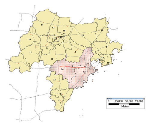
Using the Jinan–Qingdao South Expressway Project in Shandong Province, China, as an example in this study, the area was divided into 24 regions to study the economic driving and induced traffic volume along the regional economy 10 years after project completion. Population, economic and other data were obtained from the Shandong Provincial Bureau of Statistics. The road network and impedance data were derived from a GIS. The traffic volume of the expressway OD and the traffic volume generated by the expressway in each region were derived from the expressway toll station and gantry passing data.
The Jinan–Qingdao South Expressway was fully completed in 2014; it passes through Zhucheng City, Jiaozhou City and the Huangdao District. The study section and area are shown in Figure 4.
6.1. Data Analysis
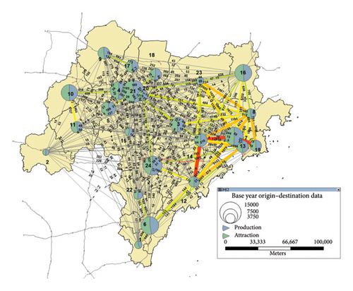
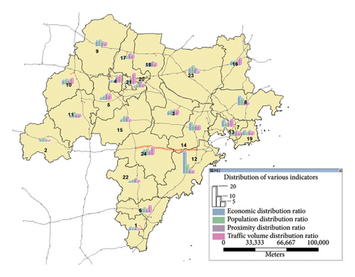
When predicting the induced traffic volume, the ESE gravity model requires the spillover economy to be quantified and the economic connection parameters to be calculated, based on the economic population, base-year distribution of the traffic volume and trend distribution of the traffic volume.
Figures 5 and 6 show the distributions of the parameters in each region when there is no project. According to the preliminary settlement results, the new roads in all 24 regions mainly affected regions 12, 14, 15, 22 and 24 (subsequently replaced by the symbols A, B, C, D and E, respectively). The cost matrices for the main affected areas are presented in Table 3 and 4.
| Region i/j | A | B | C | D | E |
|---|---|---|---|---|---|
| A | 30.71 | 57.48 | 58.18 | 70.81 | |
| B | 30.71 | 59.8 | 62.92 | 64.64 | |
| C | 57.48 | 59.8 | 34.13 | 22.27 | |
| D | 58.18 | 62.92 | 34.13 | 25.38 | |
| E | 70.81 | 64.64 | 22.27 | 25.38 |
| Region i/j | A | B | C | D | E |
|---|---|---|---|---|---|
| A | 20.41 | 55.5 | 58.18 | 35.21 | |
| B | 20.41 | 38.34 | 62.92 | 37.54 | |
| C | 55.5 | 38.34 | 34.13 | 22.27 | |
| D | 58.18 | 62.92 | 34.13 | 25.38 | |
| E | 35.21 | 37.54 | 22.27 | 25.38 |
6.2. Analysis of Prediction Results
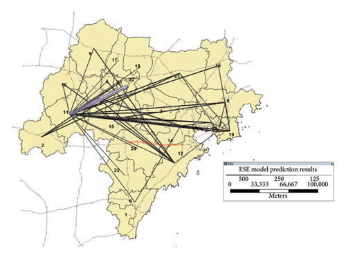
The basic data were substituted into the ESE gravity, LSTSC [6] and the T2F-LSTM models [8]. The induced traffic volume predicted by the ESE gravity model is shown in Figure 7, and the predictions for the total traffic generation by each model in conjunction with actual historical data are displayed in Figure 8.
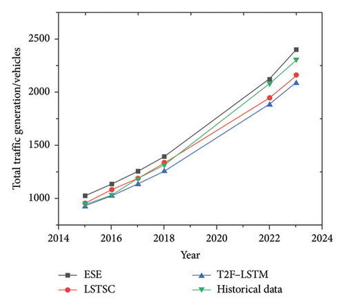
According to the results shown in Figure 8, the predictions obtained by the ESE gravity model are slightly larger than the actual historical data. This is mainly because, when there are projects, the ESE gravity model recalculates the economic connections and occurrences between regions based on the improvement in accessibility. When the cost between two regions is reduced, the economic connections and occurrences are revised upward and substituted into the model calculation to simulate the impact of the new highway on the regional economy and the driving of traffic volume. Conversely, the LSTSC and T2F-LSTM models predict by identifying the phased changes in historical trends without considering the driving effect of the economy on traffic, resulting in predictions slightly lower than the actual historical data. The mean absolute error (MAE) predictions of the ESE gravity model and LSTSC fluctuate within 10%, while the MAE predictions of the T2F-LSTM model fluctuate within 15%.
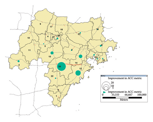
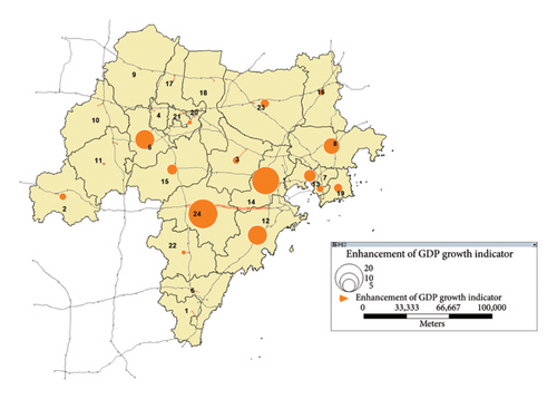
The parameters affecting the results of the ESE model are shown in Figures 9 and 10, and the main parameters of the affected areas are listed in Tables 5 and 6.
| Accessibility/region | A | B | C | D | E |
|---|---|---|---|---|---|
| Accessibility improvement (%) | 3.97 | 23.67 | 4.78 | 9.33 | 1.71 |
| Area | A | B | C | D | E |
|---|---|---|---|---|---|
| Economic drive (RMB 100 mn) | 4.02 | 22.15 | 19.86 | 11.41 | 1.12 |
The economic sensitivity calculation results for the main affected areas are listed in Table 7.
| Label | A | B | C | D | E |
|---|---|---|---|---|---|
| ESE gravity model | 15.93 | 13.97 | 1.63 | 17.95 | 73.96 |
| LSTSC model | 5.1 | 5.91 | 0.84 | 7.57 | 22.35 |
| T2F-LSTM model | 8.1 | 7.91 | 0.65 | 4.57 | 20.35 |
Table 7 shows that the sensitivity of the ESE gravity model’s economic prediction results is significantly higher than those of the LSTSC and the T2F-LSTM models. The prediction results of the ESE gravity model indicate that when the economic ties between two regions increase, more traffic links are generated between the two locations. This result is consistent with the role of highway projects in promoting regional economic development.
7. Conclusions
This study refers to the relevant theories of spatial econometrics based on which an ESE gravity model was developed aimed at assessing the potential ESEs of a new expressway on the regions along its route. The model takes into account the development patterns of induced traffic volume and the actual economic development of adjacent areas and introduces the intensity of interregional economic ties and the level of regional economic development aiming to the provision of a reference for the feasibility of engineering projects in the early stages. Related to this, the ESE gravity model was applied to predict the economic impact of engineering projects.
In analysing the potential economic effects on interregional traffic after the completion of the project, the gravity model that was based on economic spillover benefits offered a new perspective. Compared with other models, this model shows higher computational results and sensitivity to economic changes in certain cases, with the MAE value of the prediction results varying within 10%.
Analyses showed that we also recognise the challenges and limitations of the ESE gravity model. For instance, regional economies are influenced by various factors, such as economic structure, industrial structure and the state of industrial development, leading to varying degrees of economic driving on traffic across different regions, which directly affects the accuracy of model predictions. Moreover, the division of research areas is constrained by the ability to obtain data; divisions that are too detailed may result in the absence of key data, while divisions that are too broad may lead to imprecise prediction results. Therefore, the findings of this study should be interpreted in the context of these limitations and further refined in future research.
Conflicts of Interest
The authors declare no conflicts of interest.
Funding
This work was supported by the National Natural Science Foundation of China (Identification of Driver Safety for Hazardous Material Vehicles based on Visual Characteristics, grant number 52102412), 2021 Shandong Provincial Natural Science Foundation (Project/Research on Urban Traffic Control in a Hybrid Environment of Intelligent Connected Vehicles, grant number ZR2021MF019), 2021 Shandong Provincial Natural Science Foundation Project (Youth Fund) (Research on Dynamic Activation Determination Mechanism and Rapid Diversion Control Method of Urban Traffic Network Bottleneck Areas, project number: ZR2021QF110), Shandong Provincial Department of Science and Technology (New Generation Information Technology) (Research on New Architecture and Key Technologies of Hybrid Enhanced Intelligent ‘Transportation Brain’, project number: 2021TSGC1011), Shandong Provincial Department of Science and Technology (New Generation Information Technology) (Key Technology Research and Application of Smart Tunnel Integrated Safety Supervision Platform, project number 2022TSGC20962022-11 to 2024-11), Shandong Province Social Science Planning and Research Project (Study on the Coupling Mechanism and Implementation Path of Carbon Peak Driving Factors in the Transportation Sector of Shandong Province, grant number 22CJJJ31) Shandong Province Key R&D Programme (Soft Science) Key Project (grant number 2023RZB06052), Jinan City’s Self Developed Innovative Team Project for Higher Educational Institutions (grant number 20233040), Shandong Provincial Department of Science and Technology (New Generation Information Technology) (Research and Development of an Intelligent Urban Public Transportation Dispatch System based on Multisource Data Fusion, project number: 2023TSGC0158) and Shandong Provincial Department of Industry and Information Technology (New Generation Information Technology Project), project name: Research on New Architecture and Key Technologies of Hybrid Enhanced Artificial Intelligence ‘Traffic Brain’, project number: 202160101683.
Acknowledgements
The author acknowledges that the Department of Transportation and Logistics Engineering at Shandong Jiaotong University and the Shandong Key Laboratory of Smart Transportation (Preparation) provided the materials and resources necessary to achieve the set goals.
Supporting Information
Supporting information contains model predictions for all regions.
Open Research
Data Availability Statement
The data that support the findings of this study are available from the corresponding author upon reasonable request.


