Accurate modelling of gastric evacuation (GE) is a prerequisite for optimising feeding strategies in aquaculture and improving predator–prey interaction models in ecological studies. However, GE analysis is challenging because of the interdependencies of the variables influencing the evacuation process. To overcome this, a general power function was developed in 1992 and refined in 1998 using non-linear regression techniques. The proposed method is robust for identifying the best-fit evacuation function while simultaneously assessing the effects of potential predictor variables. This study demonstrated the application of R statistical software for parameter estimation of the general power function to characterise the influence of fish size, meal size and temperature on GE rate (GER) in brown trout (Salmo trutta Linnaeus, 1758) and rainbow trout (Oncorhynchus mykiss Walbaum, 1792). The statistical methods presented are remarkably adaptable and applicable to a wide range of GE datasets. Furthermore, they can be extended to incorporate additional variables influencing GE, making them integral tools for advancing research in fisheries management, ecological modelling and aquaculture.

1. Introduction

Accurate estimation of gastric evacuation rates (GERs) is a prerequisite for understanding fish digestion and feeding dynamics, with significant implications for aquaculture, ecological studies and physiological research [1–3]. In aquaculture, precise gastric evacuation (GE) data can be used to enhance feeding efficiency, ensuring optimal nutrient utilisation while minimising waste [4–6]. The integration of automatic feeder systems represents a promising technological advancement, as it allows for the refinement of feeding strategies based on accurate GER estimations [7–9]. Such optimisation can reduce operational costs and mitigate the environmental impacts associated with uneaten food and overfeeding, such as water pollution [10, 11]. The effectiveness of these systems strongly depends on the accurate incorporation of GER into the design of feeding frequencies that achieve optimal outcomes [7–9]. Conversely, reliance on inaccurate GER data can lead to underfeeding or overfeeding, resulting in suboptimal growth, compromised fish health and environmental degradation due to excessive nutrient discharge [12–15]. In ecological contexts, inaccurate GER data can distort estimates of predator food consumption rates, leading to misinterpretations of predator feeding behaviour and its impact on prey populations [16–19]. Such inaccuracies may have broader implications, potentially affecting assessments of food web interactions, trophic relationships and overall ecosystem stability [20, 21]. Consequently, obtaining precise GER data from controlled experiments and accurately modelling these data are essential for supporting reliable predictions and informed management decisions in both aquaculture and ecological studies [3, 22, 23].

The first critical step in accurately determining GER for a fish involves selecting an appropriate function that adequately describes the relationship between the stomach contents and postprandial time [24–27]. However, the selection of an appropriate function remains a topic of debate, with various functions, such as linear, square root, surface area-dependent and exponential, being employed to describe GE in fish [3, 16, 28, 29]. The GER and total evacuation times predicted by these functions often differ considerably. For instance, the linear function tends to underestimate GER for larger meals and overestimate it for smaller ones, whereas the surface area-dependent and exponential functions exhibit opposite trends [22]. In contrast, the square root function consistently reflects the GER patterns across datasets with varying meal sizes. This consistency was supported by the mechanistic cylinder model, which attributes it to anatomical factors such as constant stomach length and proportional expansion of the mucosal surface area with increasing stomach content [30]. This model conceptualises stomach content as a cylinder that gradually reduces in its mass through successive peeling of its sides, while the ends remain largely unaffected [30, 31]. This geometric interpretation further substantiates the square root function’s suitability for accurately modelling GE in fish.

The general power function, developed by Temming and Andersen [32] based on the suggestions of Tyler [33] and Jones [34], was fully established in non-linear regression by Temming and Andersen [35]. Andersen [36] later refined the function to ensure its applicability in describing GE independently of meal size. The power function is expressed in a form where the power exponent α determines the evacuation pattern. Notably, when α ≈ , the function simplifies to a square root function, which has been widely applied to describe GER independently of meal size [30, 35]. Furthermore, experimental evidence suggests that deviations of α from may indicate prey heterogeneity, with values below pointing to digestion delays due to structurally resistant prey like crustaceans with robust exoskeletons and values above reflecting an initially high GER due to rapid evacuation of less resistant materials (e.g., fish fins, head regions and entrails), while more structurally intact components (e.g., the trunk) persist longer in the stomach [37]. The flexibility of the general power function allows it to accommodate prey characteristics (e.g., dietary energy density and disintegration stability), while also accounting for key variables such as body size and temperature [4, 37, 38]. Given its adaptability, the general power function is the most suitable approach for modelling GE because it allows for identifying the best-fit function while simultaneously parameterising the effects of multiple variables on GER.

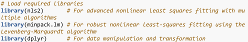
The general power function is implemented using the nls and nlsLM functions in R statistical software, available through the stats and minpack.lm packages [39, 40], which estimate parameters for non-linear models. These functions employ iterative optimisation methods, with nls relying on the Gauss–Newton algorithm and nlsLM utilising the more robust Levenberg–Marquardt algorithm. Their flexibility allows for the accurate estimation of complex non-linear relationships, making them valuable tools for analysing GE processes [41, 42]. Given R’s widespread use in academic research, these statistical approaches can be broadly applied to GE modelling [43].

The present study aimed to present and demonstrate the use of R scripts for the general power function using GE data from brown trout (Salmo trutta Linnaeus, 1758) [5] and rainbow trout (Oncorhynchus mykiss Walbaum, 1792) [6] as sample datasets. This study provided a comprehensive guide on: (1) selecting the best-fit function for GE data, (2) examining the effects of body size and temperature as potential variables influencing GER and (3) modelling the optimum and upper thermal limits for rainbow trout. Additionally, this study used the parametrised GER model to generate GE curves for brown and rainbow trout, depicting the relationship between stomach contents (S_t, in grammes) and postprandial time (t, in h). The statistical procedures outlined in this study can be applied to various GE datasets and readily expanded to incorporate other variables influencing the GE process across different fish species.

2. Materials and Methods

2.1. Selection of the Best-Fit Function

The general power function was used to determine the best-fit function for describing the GE pattern, independently of meal size. The function is expressed as follows:

(1)

This equation is integrated over time from meal ingestion at t = 0 to t as follows:

where S_t represents the stomach content mass (g) at postprandial time t following the ingestion of a meal of mass S₀ (g). The parameter ε is a normally distributed variable, ρ denotes the rate parameter (g^1−α h⁻¹), and α is the power parameter that characterises the pattern of food evacuation from the stomach. The selected function depends on the value of α:

•
If α = 0, the function becomes linear, indicating a steady GER.
•
For α = , the function is the square root with GER slowing down over time.
•
When α = , the function is surface area-dependent, suggesting that the evacuation depends on the surface area of the food and that the food items decrease isometrically.
•
If α = 1, the function becomes exponential, indicating that the GER depends solely on the prey mass.

The standard deviation of the random error term ε increases linearly with meal size S₀; thus, the GER data relative to meal size standardises the variance so that each observation is equally weighted. In the general power model, a weighting factor of is used to adjust for variability solely due to differences in meal sizes. However, this adjustment remedies only the heterogeneity stemming from different meal sizes; it does not necessarily account for the additional variance that develops over time during evacuation [44]. In R, this weighting factor can be applied in the nls() function by specifying , ensuring variance adjustment for differences in meal sizes. It should be noted that, in this paper, such a weighting factor was not applied.

2.2. Temperature and Fish Size Effects on GER

The rate parameter ρ in the general power function can be extended to account for the effects of various variables on GER. Here, as an example, the effects of two variables, that is, fish size and temperature, on GER are examined.

A simple power function was employed to parameterise the influence of fish size L [29] as follows:

(2)

To explore the influence of temperature T, an exponential function was employed:

(3)

where λ, δ and α are the parameters to be estimated.

2.3. Optimum and Upper Thermal Limit Modelling

The parameterisation of the effects of temperature on GER is typically determined by a simple exponential function. While this approach is suitable for lower-temperature ranges, it is inadequate for higher-temperature ranges. Several species, including Atlantic cod (Gadus morhua Linnaeus, 1758) [33, 38], Atlantic herring (Clupea harengus Linnaeus, 1758) [45], European sprat (Sprattus sprattus Linnaeus, 1758) [46], brook trout (Salvelinus fontinalis Mitchill, 1814) [4] and rainbow trout [6], exhibit optimal temperatures for their GER within the upper temperature range. Beyond this range, the GER decreases significantly and eventually reaches zero. The application of the optimum temperature function proposed by Andersen [38] allows for the determination of both the optimum and upper temperature limits for GER in fish. Consequently, Equation (3) has alternatively been described as follows:

(4)

where δ₁ and δ₂ are temperature coefficients and T_u is the upper temperature limit at which the GER is zero.

The GE data for brown trout [5] and rainbow trout [6] were used as sample datasets to apply the general power function in R statistical software. These studies found that the estimated power parameter α for both fish species was close to

, suggesting that the square root function effectively describes the GE process in these species. As a result, the square root function was used in the subsequent data analysis to model the GE as follows:

(5)

This equation is integrated over time from meal ingestion (t = 0) into t:

Normality and variance homogeneity, which are critical for model validity, were thoroughly discussed by Andersen [3], who derived and validated the variance structure for the square root function. Remedies for heteroscedasticity, such as applying a weighting factor of in non-linear regression on the square root function, are also detailed in Andersen [3], particularly when multiple predictor variables are involved complicating use of the maximum likelihood (ML) approach. In R statistical software, this remedy can be incorporated by specifying a weighting factor in the nls() function using weights = (ρ × time)⁽⁻²⁾. Statistical tests such as the Shapiro–Wilk, Breusch–Pagan or White’s test can be used to assess these assumptions, while residual pattern analysis remains essential for verifying independence [47]. Again, note that, in this paper, such a weighting factor was not applied.

2.4. Effects of Temperature and Fish Size on GER

The rate parameter in Equation (5) can be further extended to account for the influences of body size and temperature, as demonstrated in Equations (2–4):

(6)

(7)

(8)

The parameter values for the aforementioned equations were estimated using R statistical software (v. 4.3.3; 39) within the RStudio interface (v. 2024.12.0; [48]). Non-linear regression analyses were performed using the nls function [39] or nlsLM function [40] to ensure robust parameter estimation. Data manipulation and preprocessing were performed using the dplyr package [49]. The parameters used in the equations and their corresponding notations in the R script for the computational implementation are given in Table 1.

Table 1. Symbols for variables and parameters and their corresponding notations in the R script.

Symbol	Explanation	Representation in R script
	Experiment number	expno
T	Temperature in °C	temp
L	Fish total length (cm)	predlcm
W	Fish total weight (g)	predw
S₀	Meal size consumed by the fish	sow
S_t	Stomach content weight (g) at time t	stw
t	Postprandial time (in h)	time
α	Shape exponent	B
λ	Length exponent	C
δ	Temperature coefficient; Equations (3) and (5)	A
δ₁	Temperature coefficient; Equations (4) and (8)	A1
δ₂	Temperature coefficient; Equations (4) and (89)	A2
ρ	Rate parameter constant; Equations (1) and (5)	R
ρ_L	Rate constant; extended to account for the effect of L; Equations (2) and (6)	RL
ρ_T	Rate constant; extended to account for the effect of T	RT
ρ_LT	Rate constant; extended to account for the effects of L and T; Equations (3), (4), (7) and (8)	RLT

2.5. Sample Dataset

The GE data for brown trout from Dürrani and Seyhan [5] (expno 1–5) and rainbow trout (expno 6–14) from Dürrani [6], which was saved in a comma-separated values (csv) file, was used in R statistical software. The sample dataset “GER_data.csv” can be retrieved from GitHub repository (see the “Data Availability Statement” section).

Install these packages and run the following steps:

To load the dataset “GER_data.csv” in R statistical software, the following code was used:

3. Results

3.1. Example 1: Selection of Best-Fit Function

In R statistical software, Equation (1) was applied to the first two GE experiments on brown trout by Dürrani and Seyhan [5] at 17.5°C to identify the best-fit function for describing their GE pattern.

The R script for Equation (1) is structured as follows:

The complete R script for Equation (1) of the general power function is integrated and executed as follows:

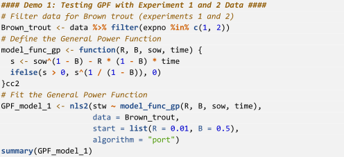
The output from the R statistical software for the general power function (Equation (1)) is summarised in Figure 1.

Details are in the caption following the image — **Figure 1**
Open in figure viewer PowerPoint

Summary statistics for the parameter estimation of the general power function , as provided by R statistical software. Table 1 lists the parameters used in the function and their corresponding symbols in the R script.

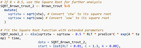
3.2. Example 2: Square Root Function

The estimated value of the power parameter α (B = 0.498) was close to , indicating that the square root function adequately describes the GE process in brown trout. As a result, the GE data of brown trout were reanalysed using the square root function, Equation (5), as follows:

In R statistical software, Equation (5) can be expressed as follows:

Prior to running the square root function, the initial stomach content (S₀) and stomach contents at time t (S_t), labelled as sow and stw in the “GER_data.csv” file, need to be square-rooted as follows:

The complete R script for Equation (5) of the square root function is then integrated and executed as follows:

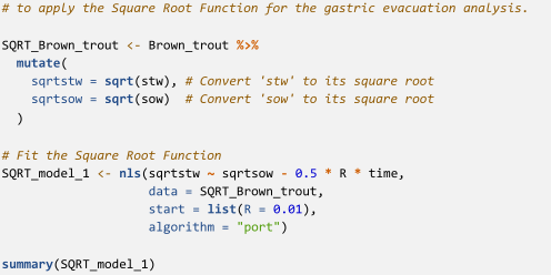
The output from the R statistical software for the square root function (Equation (5)) is summarised in Figure 2.

3.3. Example 3: Effects of Body Size and Temperature on GER Using General Power Function

Equation (3) of the general power function was applied to the GE experiments of brown trout [5] to identify the best-fit function for describing the pattern of GE in brown trout and to parameterise the effects of body size and temperature on GER. The parameters of Equation (3) were determined using the GE dataset of brown trout, which included both large and small fish fed on various meal sizes at water temperatures ranging from 13.0 to 19.2°C.

In R statistical software, Equation (3) of the general power function is expressed as follows:

The complete R script for Equation (3) of the general power function was integrated and executed as follows:

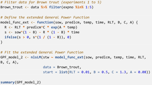
The output produced by R statistical software based on the code representing the general power function (Equation (3)) is shown in Figure 3.

3.4. Example 4: Effects of Body Size and Temperature on GER Using the Square Root Function

The estimated value of the power parameter α (B = 0.462) in Equation (3) of the general power function reaffirmed the suitability of the square root function for GE data from brown trout. Subsequently, the effects of temperature and body size on the GER of brown trout were reanalysed using Equation (7) of the square root function.

In R statistical software, Equation (7) of the square root function is expressed as follows:

The complete R script for Equation (7) of the square root function was integrated and executed as follows:

The output generated by R statistical software for the square root function (Equation (7)) is summarised in Figure 4.

The parametrised GER model for brown trout, including the estimated values of ρ_LT, λ and δ is provided in Equation (7):

(9)

In Equations (3) and (7), the effects of water temperature on the GER of brown trout were modelled using a simple exponential function, as Dürrani and Seyhan [5] did not observe an optimum temperature for this fish within the tested range of 13.0 to 19.2°C. Consequently, the dataset for rainbow trout [6] was used to execute Equations (4) and (8), as an optimum temperature for this species has been reported.

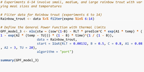
3.5. Example 5: Optimum and Upper Thermal Limits Modelling With a General Power Function

The GE data for rainbow trout [6], which included fish of various sizes fed different meal sizes composed of commercial pellets at water temperatures ranging from 7.8 to 19.2°C, were used to determine the parameters of the general power function. This analysis incorporated the temperature function proposed by Andersen [38].

In R statistical software, Equation (4) of the general power function is expressed as follows:

Complete R script for Equation (4) of the general power function, incorporating Andersen’s [38] temperature function, was integrated and executed.

The output generated by R statistical software for the general power function (Equation (4)) is summarised in Figure 5.

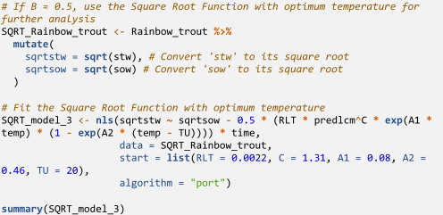
3.6. Example 6: Optimum and Upper Thermal Limits Modelling With the Square Root Function

The estimated value of the power parameter α (B = 0.509) was close to , which suggests that the square root function also best describes the GE process in rainbow trout. Consequently, the GE data for rainbow trout were reanalysed using Equation (8) of the square root function, incorporating Andersen’s [38] temperature function.

In R statistical software, Equation (8) of the square root function, incorporating Andersen’s [38] temperature function, is represented as follows:

The complete R script for Equation (8) representing the square root function was integrated and executed as follows:

The output generated by R statistical software for the square root function (Equation (8)) is summarised in Figure 6.

Using the estimated values of ρ_LT, λ and δ, the parameterised form of Equation (8) can be obtained as follows:

(10)

Dürrani [6] fixed the value of the first temperature coefficient, δ₁ (denoted as A1 in the R script), at 0.08. The corresponding results generated by R statistical software are presented in Figure 7. For further details on fixing the temperature coefficient at 0.08, refer to Andersen [38].

Consequently, the parameterised form of Equation (8) proposed by Dürrani [6] is as follows:

(11)

This parametrised GER model was used to determine the optimum and upper thermal limits for the GER of rainbow trout. The model demonstrates an exponential increase in GER with rising temperature, peaking at 18.6°C, with an evacuation rate parameter of 6.285 × 10⁻³. However, as the temperature exceeded 18.6°C, the GER declined sharply, eventually reaching zero at 20.9°C, indicating the complete cessation of GE.

3.7. Example 7: Constructing XY Plots Indicating the Optimum and Upper Thermal Limits

In this example, the length exponent λ is fixed at 0.75 in Equation (6) of the square root function, which is expressed as .

This equation was used to estimate the rate parameter constant ρ_L for each individual GE experiment conducted on the rainbow trout, as summarised in Figure 8.

In R statistical software, Equation (6) of the square root function is expressed as follows:

The rate parameter constant ρ_L for each individual experiment indicates an increase in the GER from 3.13 × 10⁻³ at 7.8°C to 5.28 × 10⁻³ at 15°C (Figure 8). Subsequently, Equation (7), , is applied to determine the effects of temperature within the lower range, covering experiments 6–11 (Figure 9). It should be noted that this step is optional and is not necessary to determine the optimum and upper temperature limits; it serves only as an illustration. The exponential function predicts a continuous increase in GER with increasing temperature, which is physiologically implausible.

The rate parameter constant ρ_L for each individual experiment was plotted against the temperature and two curves were provided: the exponential curve (- - - - -) is provided by the use of ρ_L = 0.00171e^0.072T, while the optimum temperature curves (—) are provided by the use of ρ_LT = 0.00152e^0.08T(1 − e^{1.18(T − 20.90)}) (Figure 10).

3.8. Example 8: Constructing XY Plots With GE Curves Using a Parametrised GER Model

In this example, the parameterised GER models for brown trout (Equation (9)) and rainbow trout (Equation (11)) are used to generate GE curves for individual GE experiments, demonstrating the procedure in an Excel sheet.

Equation (9) was used to generate the GE curve for brown trout, with fish averaging 30 cm in total length fed a 6 g meal of commercial pellets at 17.5°C (Figure 11a). Similarly, Equation (11) was applied to rainbow trout, in which fish of the same length received 7 g of meal at 19.2°C (Figure 11b).

To illustrate the GE process, the weight of stomach contents (g) recovered at various postprandial times t is plotted on the Y-axis, while the corresponding recovery time t is plotted on the X-axis. The parametrised GER model is then used to generate the GE curve, depicting the relationship between stomach contents (g) and the elapsed time t. This visualisation effectively demonstrates how stomach contents decrease over time as the fish digests its meal. The GE curve, which was derived from the parametrised GER model, provides valuable insights into the digestion process by clarifying the rate at which the stomach evacuates its contents.

4. Discussion

This study presents the first comprehensive guide for analysing GE data using the general power function in R statistical software. A key advantage of the R statistical software’s nls function lies in its flexibility for accommodating diverse models, enhancing its applicability across datasets [41, 42]. Reanalysis of GE data from brown trout [5] and rainbow trout [6] using this software reaffirmed the superior fit of the square root function, which accurately describes the course of GE independently of meal size. The square root model’s utility has been validated for multiple wild fish species, including saithe (Pollachius virens Linnaeus, 1758), whiting (Merlangius merlangus Linnaeus, 1758) and Atlantic cod, which were fed a variety of prey species [3, 22, 36, 50, 51]. Similarly, this function has proven effective in describing GE in farmed fish species such as brook trout, brown trout, rainbow trout and European seabass (Dicentrarchus labrax Linnaeus, 1758) [5, 6, 52, 53]. Furthermore, the square root function is supported by the mechanistic cylinder model, which considers surface area digestion, although meal characteristics—discussed in the Introduction section—can cause deviations that should be considered when modelling GE in predatory fish. Thus, various studies have provided strong empirical support for the application of the square root function to model GER in both farmed and wild fish.

Notably, the temperature coefficient, particularly in the optimum temperature function (δ₂) was not statistically significant (Figures 5–7). This lack of significance likely arises from two interrelated factors. First, the dataset is imbalanced with respect to body size and temperature, which increases variability in specific subgroups and diminishes the function’s capacity to detect a true temperature effect. Second, the narrow gap between the two highest temperature groups may mask subtle changes in GER, as the physiological response appears to plateau near the upper temperature limit. These findings are consistent with Andersen [38], who observed similar issues even with balanced data when the upper temperature range was limited. Future research should consider expanding the temperature range and addressing data imbalances to more accurately capture the temperature-dependent behaviour of GE.

The general power function offers a promising approach for modelling GE and may have potential applications beyond fish, extending to other animal species. Future studies should explore this possibility to evaluate its broader relevance in digestive physiology. If empirical data from non-fish species indicate functions other than the square root, researchers should readily adjust parameters in the R script to transition between the functions (Figure 12). Consequently, the ability to transition between functions and integrate additional predictors should enable researchers to model diverse GE processes. For example, Equation (8) can be extended to parameterise the effect of dietary energy on GER:

In R statistical software, this equation can be expressed as follows:

Although the general power function provides a robust statistical framework, stage-dependent mechanistic approaches rooted in the basic square root function, such as the method applied by Andersen, Chabot, and Couturier [50] to model crustacean prey evacuation, are strongly recommended over transitioning between functions. This approach can address inherent limitations of purely statistical methods, that is, Couturier et al. [37], which may oversimplify physiological processes, particularly in prey species with distinct digestion phases. Although a full exploration of mechanistic models falls outside the scope of this study, their utility for capturing biological realism in complex systems is emphasised.

Additionally, established statistical software conversion tools (e.g., CodeConvert AI: www.codeconvert.ai) enable efficient translation of R scripts into formats compatible with other widely used statistical platforms, such as SAS or Python. This capability ensures that methodologies developed in R can be readily adapted and implemented across alternative software environments, thereby, enhancing the accessibility and applicability of this study.

5. Conclusions

This study offers a practical guide to modelling GER in fish using the general power function, with a particular emphasis on parameter estimation and analysis using R statistical software. This approach should simplify and enhance the efficiency of the GER modelling process. The results suggest that the general power function provides a robust and versatile framework for GER modelling, with applications across diverse statistical environments. This methodology can advance research on GE while also deepening our understanding of digestive efficiency and metabolic responses in fish. Furthermore, these findings are expected to provide a solid foundation for future research, enabling the exploration of GER across various species and environmental conditions, which could drive further progress in the field.

Conflicts of Interest

The author declares no conflicts of interest.

Funding

The author declare that no funds, grants or other support were received for this study.

Open Research

Data Availability Statement

The R script and sample dataset (gastric evacuation data) used in this study are available in the GitHub repository: https://github.com/OmerhanDurrani/Modelling_GER. This repository also includes a detailed procedure for constructing Figures 10 and 11, provided in Microsoft Excel format.

References

1 Bajkov A. D., How to Estimate the Daily Food Consumption of Fish under Natural Conditions, Transactions of the American Fisheries Society. (1935) 65, no. 1, 288–289, https://doi.org/10.1577/1548-8659(1935)65%5b288:HTETDF%5d2.0.CO;2, 2-s2.0-84946643986.
10.1577/1548-8659(1935)65[288:HTETDF]2.0.CO;2
Google Scholar
2 Jobling M., Aspects of Food Consumption and Energy Metabolism of Farmed Plaice, Pleuronected Platessa L, 1978, University of Glasgow (United Kingdom), ProQuest Dissertations & Theses.
Google Scholar
3 Andersen N. G., The Dynamics of Gastric Evacuation in Predatory Fish: A Mechanistic Model of Gastric Evacuation – Development and Applications in Fish and Fishery Biology, DTU Orbit, Lyngby, Denmark, 39–41, 2022, (Doctoral Thesis).
Google Scholar
4 Dürrani Ö. and Seyhan K., Gastric Evacuation Rates in Farmed Brook Trout Subjected to a Range of Feeding Conditions Fed Commercial Pellets, Aquaculture. (2019) 513, https://doi.org/10.1016/j.aquaculture.2019.734390, 2-s2.0-85070617343, 734390.
10.1016/j.aquaculture.2019.734390
Web of Science® Google Scholar
5 Dürrani Ö. and Seyhan K., Parameterizing an Expanded Square Root Model to Account for the Effects of Temperature, Meal Size, and Body Size on Gastric Evacuation Rate in Farmed Brown Trout, Aquaculture Research. (2021) 52, no. 10, 4849–4857, https://doi.org/10.1111/are.15318.
10.1111/are.15318
Web of Science® Google Scholar
6 Dürrani Ö., Temperature, Meal Size and Body Size Effects on the Gastric Evacuation of Rainbow Trout: Modelling Optimum and Upper Thermal Limits, Journal of Fish Biology. (2022) 100, no. 6, 1388–1398, https://doi.org/10.1111/jfb.15049.
10.1111/jfb.15049
PubMed Web of Science® Google Scholar
7 Handeland S. O., Imsland A. K., and Stefansson S. O., The Effect of Temperature and Fish Size on Growth, Feed Intake, Food Conversion Efficiency and Stomach Evacuation Rate of Atlantic Salmon Post-Smolts, Aquaculture. (2008) 283, no. 1–4, 36–42, https://doi.org/10.1016/j.aquaculture.2008.06.042, 2-s2.0-51049122129.
10.1016/j.aquaculture.2008.06.042
Web of Science® Google Scholar
8 Jia Y., Gao Y., Jing Q., Huang B., Zhai J., and Guan C., Gastric Evacuation and Changes in Postprandial Blood Biochemistry, Digestive Enzymes, and Appetite-Related Genes in Juvenile Hybrid Grouper (Epinephelus moara ♀ × E. lanceolatus ♂), Aquaculture. (2021) 530, https://doi.org/10.1016/j.aquaculture.2020.735721, 735721.
10.1016/j.aquaculture.2020.735721
CAS Web of Science® Google Scholar
9 Gilannejad N., Silva T., Martínez-Rodríguez G., and Yúfera M., Effect of Feeding Time and Frequency on Gut Transit and Feed Digestibility in Two Fish Species With Different Feeding Behaviours, Gilthead Seabream and Senegalese Sole, Aquaculture. (2019) 513, https://doi.org/10.1016/j.aquaculture.2019.734438, 2-s2.0-85072087604, 734438.
10.1016/j.aquaculture.2019.734438
CAS Web of Science® Google Scholar
10 Zhou C., Xu D., Lin K., Sun C., and Yang X., Intelligent Feeding Control Methods in Aquaculture With an Emphasis on Fish, Reviews in Aquaculture. (2018) 10, no. 4, 975–993, https://doi.org/10.1111/raq.12218, 2-s2.0-85056309199.
10.1111/raq.12218
Web of Science® Google Scholar
11 Li D., Wang Z., Wu S., Miao Z., Du L., and Duan Y., Automatic Recognition Methods of Fish Feeding Behavior in Aquaculture: A Review, Aquaculture. (2020) 528, https://doi.org/10.1016/j.aquaculture.2020.735508, 735508.
10.1016/j.aquaculture.2020.735508
Web of Science® Google Scholar
12 Riche M., Haley D. I., Oetker M., Garbrecht S., and Garling D. L., Effect of Feeding Frequency on Gastric Evacuation and the Return of Appetite in Tilapia Oreochromis Niloticus (L.), Aquaculture. (2004) 234, no. 1–4, 657–673, https://doi.org/10.1016/j.aquaculture.2003.12.012, 2-s2.0-1842866907.
10.1016/j.aquaculture.2003.12.012
Web of Science® Google Scholar
13 Lee S.-M., Hwang U.-G., and Cho S. H., Effects of Feeding Frequency and Dietary Moisture Content on Growth, Body Composition and Gastric Evacuation of Juvenile Korean Rockfish (Sebastes Schlegeli), Aquaculture. (2000) 187, no. 3-4, 399–409, https://doi.org/10.1016/S0044-8486(00)00318-5, 2-s2.0-0034691956.
10.1016/S0044-8486(00)00318-5
Web of Science® Google Scholar
14 Oliveira F. A., Argentim D., Novelli P. K., Agostinho S. M. M., Agostinho L. M., and Agostinho C. A., Automatic Feeders for Nile Tilapia Raised in Cages: Productive Performance at High Feeding Frequencies and Different Rates, Arquivo Brasileiro de Medicina Veterinária e Zootecnia. (2016) 68, no. 3, 702–708, https://doi.org/10.1590/1678-4162-7882, 2-s2.0-84977538854.
10.1590/1678-4162-7882
CAS Web of Science® Google Scholar
15 Føre M., Alver M. O., Frank K., and Alfredsen J. A., I. Kyriazakis, Advanced Technology in Aquaculture—Smart Feeding in Marine Fish Farms, Chapter 9 In Smart Livestock Nutrition, 2023, Springer International Publishing, Cham, 227–268, Smart Animal Production.
Google Scholar
16 Bromley P. J., The Role of Gastric Evacuation Experiments in Quantifying the Feeding Rates of Predatory Fish, Reviews in Fish Biology and Fisheries. (1994) 4, no. 1, 36–66, https://doi.org/10.1007/BF00043260, 2-s2.0-0028585225.
10.1007/BF00043260
Web of Science® Google Scholar
17 He E. and Wurtsbaugh W. A., An Empirical-Model of Gastric Evacuation Rates for Fish and an Analysis of Digestion in Piscivorous Brown Trout, Transactions of the American Fisheries Society. (1993) 122, no. 5, 717–730, https://doi.org/10.1577/1548-8659(1993)122%3C0717:AEMOGE%3E2.3.CO;2.
10.1577/1548-8659(1993)122<0717:AEMOGE>2.3.CO;2
Web of Science® Google Scholar
18 Andersen N. G. and Riis-Vestergaard J., The Effects of Food Consumption Rate, Body Size and Temperature on Net Food Conversion Efficiency in Saithe and Whiting, Journal of Fish Biology. (2003) 62, no. 2, 395–412, https://doi.org/10.1046/j.1095-8649.2003.00030.x, 2-s2.0-2342627271.
10.1046/j.1095-8649.2003.00030.x
Web of Science® Google Scholar
19 Elliott J. M. and Persson L., The Estimation of Daily Rates of Food Consumption for Fish, The Journal of Animal Ecology. (1978) 47, no. 3, 977–991, https://doi.org/10.2307/3682.
10.2307/3682
Web of Science® Google Scholar
20 da Silveira E. L., Semmar N., and Cartes J. E., et al.Methods for Trophic Ecology Assessment in Fishes: A Critical Review of Stomach Analyses, Reviews in Fisheries Science & Aquaculture. (2019) 28, no. 1, 71–106.
Web of Science® Google Scholar
21 Andersen N. G., Neuenfeldt S., Bogstad B., Andersen K. H., Beyer J. E., and Travers-Trolet M., Nutritional Status Determines Apparent Assimilative Capacity and Functional Response of Marine Predatory Fish, ICES Journal of Marine Science. (2021) 78, no. 10, 3615–3624, https://doi.org/10.1093/icesjms/fsab197.
10.1093/icesjms/fsab197
Web of Science® Google Scholar
22 Andersen N. G., A Gastric Evacuation Model for Three Predatory Gadoids and Implications of Using Pooled Field Data of Stomach Contents to Estimate Food Rations, Journal of Fish Biology. (2001) 59, no. 5, 1198–1217, https://doi.org/10.1111/j.1095-8649.2001.tb00186.x.
10.1111/j.1095-8649.2001.tb00186.x
Web of Science® Google Scholar
23 Jobling M., Arnesen A. M., Baardvik B. M., Christiansen J. S., and Jørgensen E. H., Monitoring Feeding Behaviour and Food Intake: Methods and Applications, Aquaculture Nutrition. (1995) 1, no. 3, 131–143, https://doi.org/10.1111/j.1365-2095.1995.tb00037.x, 2-s2.0-84990519202.
10.1111/j.1365-2095.1995.tb00037.x
Web of Science® Google Scholar
24 dos Santos J. and Jobling M., Factors Affecting Gastric Evacuation in Cod, Gadus Morhua, L., Fed Single-Meals of Natural Prey, Journal of Fish Biology. (1991) 38, no. 5, 697–713, https://doi.org/10.1111/j.1095-8649.1991.tb03159.x, 2-s2.0-0026305326.
10.1111/j.1095-8649.1991.tb03159.x
Web of Science® Google Scholar
25 Gao X. Q., Wang X., and Wang X. Y., et al.Effects of Different Feeding Frequencies on the Growth, Plasma Biochemical Parameters, Stress Status, and Gastric Evacuation of Juvenile Tiger Puffer Fish (Takifugu Rubripes), Aquaculture. (2022) 548, https://doi.org/10.1016/j.aquaculture.2021.737718, 737718.
10.1016/j.aquaculture.2021.737718
CAS Web of Science® Google Scholar
26 Paakkonen J. P. J. and Marjomaki T. J., Gastric Evacuation Rate of Burbot Fed Single-Fish Meals at Different Temperatures, Journal of Fish Biology. (1997) 50, no. 3, 555–563, https://doi.org/10.1006/jfbi.1996.0317, 2-s2.0-0031104706.
10.1006/jfbi.1996.0317
Web of Science® Google Scholar
27 Bascinar N. S., Bascinar N., Khan U., and Seyhan K., Effects of Meal and Body Sizes on Gastric Evacuation Rate in Brook Trout Salvelinus Fontinalis (Mitchill, 1814) Fed Commercial Pellets in Group Feeding, Indian Journal of Fisheries. (2017) 64, no. 3, 50–54.
10.21077/ijf.2017.64.3.59243-08
Web of Science® Google Scholar
28 Jobling M., C. A. Simenstad and G. M. Cailliet, Mythical Models of Gastric Emptying and Implications for Food Consumption Studies, Contemporary Studies on Fish Feeding: The Proceedings of GUTSHOP ’84, 1986, 7, Springer, Dordrecht, 35–50, Developments in Environmental Biology of Fishes.
Google Scholar
29 Jobling M., Mathematical-Models of Gastric-Emptying and the Estimation of Daily Rates of Food-Consumption for Fish, Journal of Fish Biology. (1981) 19, no. 3, 245–257, https://doi.org/10.1111/j.1095-8649.1981.tb05829.x, 2-s2.0-0019745257.
10.1111/j.1095-8649.1981.tb05829.x
Web of Science® Google Scholar
30 Andersen N. G. and Beyer J. E., Mechanistic Modelling of Gastric Evacuation in Predatory Gadoids Applying the Square Root Model to Describe Surface-Dependent Evacuation, Journal of Fish Biology. (2005) 67, no. 5, 1392–1412, https://doi.org/10.1111/j.0022-1112.2005.00834.x, 2-s2.0-33845521832.
10.1111/j.0022-1112.2005.00834.x
Web of Science® Google Scholar
31 Andersen N. G. and Beyer J. E., Gastric Evacuation of Mixed Stomach Contents in Predatory Gadoids: An Expanded Application of the Square Root Model to Estimate Food Rations, Journal of Fish Biology. (2005) 67, no. 5, 1413–1433, https://doi.org/10.1111/j.0022-1112.2005.00835.x, 2-s2.0-33845517410.
10.1111/j.0022-1112.2005.00835.x
Web of Science® Google Scholar
32 Temming A. and Andersen N. G., Modelling Gastric Evacuation in Cod, 1992, 2–4, ICES CM.
Google Scholar
33 Tyler A. V., Rates of Gastric Emptying in Young Cod, Journal of the Fisheries Research Board of Canada. (1970) 27, no. 7, 1177–1189, https://doi.org/10.1139/f70-140.
10.1139/f70-140
Web of Science® Google Scholar
34 Jones R., The Rate of Elimination of Food From the Stomachs of Haddock Melanogrammus Aeglefinus, Cod Gadus Morhua and Whiting Merlangius Merlangus, ICES Journal of Marine Science. (1974) 35, no. 3, 225–243, https://doi.org/10.1093/icesjms/35.3.225, 2-s2.0-84959739997.
10.1093/icesjms/35.3.225
Google Scholar
35 Temming A. and Andersen N. G., Modeling Gastric Evacuation Without Meal Size as a Variable—A Model Applicable for the Estimation of Daily Ration of Cod (Gadus Morhua L.) in the Field, ICES Journal of Marine Science. (1994) 51, no. 4, 429–438, https://doi.org/10.1006/jmsc.1994.1044, 2-s2.0-0028162222.
10.1006/jmsc.1994.1044
Web of Science® Google Scholar
36 Andersen N. G., The Effect of Meal Size on Gastric Evacuation in Whiting, Journal of Fish Biology. (1998) 52, no. 4, 743–755, https://doi.org/10.1111/j.1095-8649.1998.tb00817.x.
10.1111/j.1095-8649.1998.tb00817.x
Web of Science® Google Scholar
37 Couturier C. S., Andersen N. G., Audet C., and Chabot D., Prey Exoskeletons Influence the Course of Gastric Evacuation in Atlantic Cod Gadus Morhua, Journal of Fish Biology. (2013) 82, no. 3, 789–805, https://doi.org/10.1111/jfb.12005, 2-s2.0-84874791974.
10.1111/jfb.12005
CAS PubMed Web of Science® Google Scholar
38 Andersen N. G., Influences of Potential Predictor Variables on Gastric Evacuation in Atlantic Cod, Gadus Morhua, Feeding on Fish Prey: Parameterization of a Generic Model, Journal of Fish Biology. (2012) 80, no. 3, 595–612, https://doi.org/10.1111/j.1095-8649.2011.03195.x, 2-s2.0-84857690014.
10.1111/j.1095-8649.2011.03195.x
CAS PubMed Web of Science® Google Scholar
39 R Core Team, A Language and Environment for Statistical Computing, 2024, Vienna, Austria, R Foundation for Statistical Computing.
Google Scholar
40 Elzhov T. V., Mullen K. M., Spiess A.-N., and Bolker B., Minpack. Lm: R Interface to the Levenberg-Marquardt Nonlinear Least-Squares Algorithm Found in Minpack, Plus Support for Bounds, 2023, R Package Version 1.2-4" https://cran.r-project.org/web/packages/minpack.lm/minpack.lm.pdf.
Google Scholar
41 Baty F., Ritz C., Charles S., Brutsche M., Flandrois J.-P., and Delignette-Muller M.-L., A Toolbox for Nonlinear Regression in R: The Package Nlstools, Journal of Statistical Software. (2015) 66, no. 5, 1–21.
10.18637/jss.v066.i05
Web of Science® Google Scholar
42 Nash J. C. and Bhattacharjee A., A Comparison of R Tools for Nonlinear Least Squares Modeling, R Journal. (2023) 15, no. 4, 198–215.
Web of Science® Google Scholar
43 Ozgur C., Kleckner M., and Li Y., Selection of Statistical Software for Solving Big Data Problems: A Guide for Businesses, Students, and Universities, Sage Open. (2015) 5, no. 2, 1–12, https://doi.org/10.1177/2158244015584379.
10.1177/2158244015584379
Web of Science® Google Scholar
44 Krog C. and Andersen N. G., Are the Dynamics of Gastric Evacuation of Natural Prey in a Piscivorous Flatfish Different From What Is Going on in a Gadoid?, Journal of Fish Biology. (2009) 75, no. 7, 1831–1844, https://doi.org/10.1111/j.1095-8649.2009.02436.x, 2-s2.0-72249116700.
10.1111/j.1095-8649.2009.02436.x
CAS PubMed Web of Science® Google Scholar
45 Temming A., Die Quantitative Bestimmung Der Konsumtion Von Fischen. Experimentelle, Methodische Und Theoretische Aspekte (in German), 1995, Universität Hamburg Habilitationsschrift.
Google Scholar
46 Bernreuther M., Temming A., and Herrmann J.-P., Effect of Temperature on the Gastric Evacuation in Sprat Sprattus Sprattus, Journal of Fish Biology. (2009) 75, no. 7, 1525–1541, https://doi.org/10.1111/j.1095-8649.2009.02353.x, 2-s2.0-72249114019.
10.1111/j.1095-8649.2009.02353.x
CAS PubMed Web of Science® Google Scholar
47 Kutner M. H., Nachtsheim C. J., Neter J., and Li W., Applied Linear Statistical Models, 2005, 5th edition, Mcgraw-Hill/Irwin, New York..
Google Scholar
48 R Studio Team, Rstudio: Integrated Development Environment for R. Rstudio, 2020, Pbc, Boston, Ma http://www.rstudio.com/.
Google Scholar
49 Wickham H., Francois R., Henry L., Müller K., and Vaughan D., Dplyr” Dplyr: A Grammar of Data Manipulation-Rproject, 2023, R package version 1.1.4: Rproject.
Google Scholar
50 Andersen N. G., Chabot D., and Couturier C. S., Modelling Gastric Evacuation in Gadoids Feeding on Crustaceans, Journal of Fish Biology. (2016) 88, no. 5, 1886–1903, https://doi.org/10.1111/jfb.12976, 2-s2.0-84966533875.
10.1111/jfb.12976
CAS PubMed Web of Science® Google Scholar
51 Temming A. and Herrmann J.-P., Gastric Evacuation in Horse Mackerel. I. The Effects of Meal Size, Temperature and Predator Weight, Journal of Fish Biology. (2001) 58, no. 5, 1230–1245, https://doi.org/10.1111/j.1095-8649.2001.tb02282.x.
10.1111/j.1095-8649.2001.tb02282.x
Web of Science® Google Scholar
52 Dürrani Ö, Seyhan K., Başçinar N., and Başçinar N. S., Satiation Meal and the Effects of Meal and Body Sizes on Gastric Evacuation Rate in Brook Trout, Salvelinus Fontinalis, Fed Commercial Pellets, Journal of Fish Biology. (2016) 89, no. 2, 1227–1238, https://doi.org/10.1111/jfb.13021, 2-s2.0-84982994478.
10.1111/jfb.13021
PubMed Web of Science® Google Scholar
53 Bal H., Durrani U., and Seyhan K., Gastric Evacuation in European Seabass Dicentrarchus Labrax (Linnaeus, 1758), Forced-Fed on Commercial Pellets, Indian Journal of Fisheries. (2023) 70, no. 1, 25–30, https://doi.org/10.21077/ijf.2023.70.1.100596-04.
10.21077/ijf.2023.70.1.100596-04
Web of Science® Google Scholar

All articles

Modelling Gastric Evacuation Rates in Fish With a General Power Function: A Step-by-Step Guide to Parameter Estimation and Analysis Using R Statistical Software

Abstract

1. Introduction