Accurate identification of photovoltaic (PV) model parameters is crucial for the study of factors affecting PV power generation efficiency. This study addresses this challenge by introducing the enhanced RIME algorithm (ERIME). ERIME achieves a fine balance between exploration and exploitation by combining a modified soft-rime search strategy and a shared information mutation mechanism, thus ensuring population diversity. To assess the efficacy of ERIME, the recognized CEC2022 test function suite is adopted to evaluate its search performance. Furthermore, to validate the versatility of ERIME in parameter identification of PV model, we tested the proposed method on several PV models, including single diode model (SDM), double diode model (DDM), triple diode model (TDM), and multiple PV module models (PVM). An in-depth statistical analysis of the results and a comparative study with the popular existing research methods highlight the superiority of ERIME. Specifically, ERIME improves the best value metrics of SDM, DDM, and TDM by 6.63E−06, 2.28E−05, and 1.36E−04, respectively, compared to RIME and reduces the standard deviation by 2.02E−03,1.75E−03, and 1.54E−03, respectively, compared to MVO. Comprehensive results show that the proposed method has better robustness and convergence accuracy than the state-of-the-art algorithm.

1. Introduction

With the increasing concern of global mankind for environmental protection and sustainable development, the development and utilization of renewable energy have gradually become the mainstream direction of global energy transition [1]. As an important renewable energy technology, solar power has been widely recognized and promoted in recent years because of its high environmental cleanliness [2]. Photovoltaic (PV) cells [3, 4, 5] convert solar energy into electricity with the help of light and get a constant supply of energy through the power generation controller [6], which makes PV power generation a long-term usable energy source for power supply.

To ensure the optimal functioning of PV cells, precise mathematical models are imperative for elucidating the intricate behaviors exhibited by these cells in distinct scenarios and for assessing the unknown parameters inherent in their models [7, 8]. Through the meticulous evaluation of acquired PV cell parameters, it becomes feasible to discern the power generation characteristics of the PV cell, along with the identification of potential faults and manifestations of aging [9].

Evaluation of parameters in PV cells is a nonlinear optimization problem [10]. A lot of work has been done by research scholars to be able to extract the parameters of PV cells efficiently. There are two main categories [11]: mathematical optimization methods and intelligent algorithms inspired by nature. Mathematical optimization methods usually require specific problems and scenarios to be effective. They may not be applicable to some PV parameter estimation problems or may not yield optimal solutions in some cases. For example, gradient-based mathematical optimization methods require the objective to be a convex function in order to obtain a globally optimal solution [12]. Nonconvex optimization problems usually need to be transformed into convex optimization form, which will undoubtedly result in a significant loss of solution accuracy [13]. Intelligent algorithms [14] do not require cumbersome problem-specific computation and reasoning, simplify the modeling process, and are well adapted to nonlinear problems. An improved elephant herding optimization algorithm (IEHOA) [15] was proposed to extract PV cell model, which employs a fast-moving operator and an elite strategy to effectively improve the convergence speed of the algorithm and shorten the optimization time of the algorithm. An improved lion swarm optimization (ILSO) [16] was employed to solve parameter identification of PV cells; the experimental results verify the superiority and effectiveness of the method. A diversification-enhanced Harris hawks optimization (DEHHO) [17] with chaotic drifts and an opposition-based exploratory strategy to be employed for identify unknown parameters of PV model modules; the experimental results show that the proposed method is capable of providing high-quality solutions. A multiple learning backtracking search algorithm (MLBSA) [18] is adopted, which effectively solves the parameter identification problem of different PV models by introducing different learning approaches and elite chaotic local search strategies. A new adaptive teaching–learning-based optimization with experience learning referred as adaptive TLBO algorithm (ELATLBO) [19] was developed to extract single diode models (SDM), dual diode models, and single diode PV modules. An efficient sine-cosine differential gradient-based optimization method (BSDGB) [20] is proposed for the identification of unknown parameters of PV models. A chaotic improved artificial bee colony (CIABC) [21] is proposed with tent chaotic map to identify solar cell models. Additionally, there are several other popular techniques proven to be accurate for PV parameter estimation, including improved tunicate swarm optimization (ITSA) [22], modified salp swarm optimization (MSSA) [23], improved Lozi map based chaotic optimization algorithm (ILCOA) [24, 25], whippy Harris hawks optimization (WHHO) [26], springy whale optimization algorithm (SWOA) [27], termed Modified RIME (TMRIME) [28], and variant of butterfly optimization algorithm (EABOA) [29]. The contributions of the above series of algorithms are listed in Table 1. As can be seen from Table 1, all the related researches have been conducted to extract the unknown parameters of the PV model by improving the original algorithm so as to enhance the efficiency of the light energy conversion [30, 31, 32, 33, 34, 35]. The above family of algorithms provides a tractable approach to the improvement of parameter identification performance of PV models. However, there still exists a varying degree of imbalance in the exploration and exploitation phases during the search process of these algorithms, as well as the possibility of falling into local minima. In addition, unreasonable parameter settings can affect convergence speed and robustness as the algorithmic search process proceeds [36].

Table 1. A literature review on parameter extraction of different PV models.

Reference	Proposed algorithm	Models	Contribution
[15]	IEHOA	SDM, DDM, and PV Module	Employ a fast-moving operator and an elite strategy
[16]	ILSO	SDM and DDM	Combine the tent chaotic map and chaotic search strategy
[17]	DEHHO	SDM, DDM, and PV Module	Embed chaotic drifts t and an opposition-based exploratory strategy
[18]	MLBSA	SDM, DDM, and PV Module	Propose historical population information and chaotic local search strategy
[19]	ELATLBO	SDM, DDM, and PV Module	Propose experience learning strategy
[20]	BSDGB	SDM, DDM, and TDM	Propose a strategy adaptive combination of three algorithms
[21]	CIABC	SDM and DDM	Improved artificial bee colony by chaotic maps
[22]	ITSA	SDM, DDM, and PV Module	Propose a two-stage improved search strategy
[23]	MSSA	SDM, DDM, and PV Module	Propose a new position update formula
[24, 25]	ILCOA	SDM, DDM, and PV Module	Updated the algorithm with Improved Lozi map strategy
[26]	WHHO	SDM, DDM, TDM, and PV Module	Introduce elimination period to HHO
[27]	SWOA	SDM, DDM, TDM, and PV Module	A novel WOA approach is proposed
[28]	TMRIME	SDM and DDM	Integrating a Polynomial Differential Learning Operator (PDLO)
[29]	EABOA	SDM, DDM, and PV Module	Dynamical position search equation by introducing a guide factor is designed

The RIME algorithm is a newly proposed and more popular intelligent algorithm based on the physical laws of nature in recent years [37]. The RIME algorithm performs well in most optimization tasks by dynamically balancing exploration and small-scale exploitation, ensuring the breadth and depth of the search process. Its mechanism improves the accuracy and efficiency of the solution, effectively preventing performance degradation and maintaining high-quality solutions. Although the RIME algorithm has achieved promising results in some engineering fields [38, 39, 40], it has been found that RIME has fewer applications in the field of PV parameter identification and suffers from unbalanced exploration and exploitation and tendency to fall into local optimal points. In this study, an enhanced RIME algorithm (ERIME) is proposed to solve the PV parameter identification problem by combining the modified soft-rime search strategy and shared information mutation strategy, and the modified soft-rime search strategy can help to ensure the balance between exploration and exploitation and improve the solution accuracy; the shared information mutation strategy can help to increase the information exchange between population agents and guide the population to evolve in a favorable direction. To verify the effectiveness of the methods, four types of PV models are used for simulation experiments, while five methods are introduced as competitors for comparison. Through effective statistical analysis of the experimental results, the results verify that the proposed method can enhance more accurate results than the existing popular methods.

In summary, the contributions of this paper are as follows:

(1)
An ERIME is proposed by combining the modified soft-rime search strategy and shared information mutation mechanism. The search performance and solution accuracy of the proposed method is verified by the state-of-the-art test function suite, and the statistical test results show the significance of the proposed method.
(2)
A careful comparison of the proposed method with five existing state-of-the-art methods in SDM, DDM, TDM, and three PVM modeling products (Photowatt-PWP201, STM6-40/36, and STP6-120/36) is carried out to validate the effectiveness of the proposed method.
(3)
The experimental results show that the proposed method is able to obtain the best results on all PV models with several statistical indicators, such as the optimal value, the mean value, and the worst value, which are obtained through several statistical experiments. In addition, a comparison of the simulated data obtained by the proposed method with the measured data shows that the proposed method is able to identify the parameters of the PV models with a high degree of accuracy.

The rest of the paper is organized. Section 2 establish the PV problem formulation; Section 3 gives the brief description of RIME algorithm; Section 4 presents the ERIME algorithm; Section 5 gives the numeral experimental results; Section 6 presents experimental results and discussions on PV problems, and conclusions are given in Section 7.

2. PV Problem Formulation

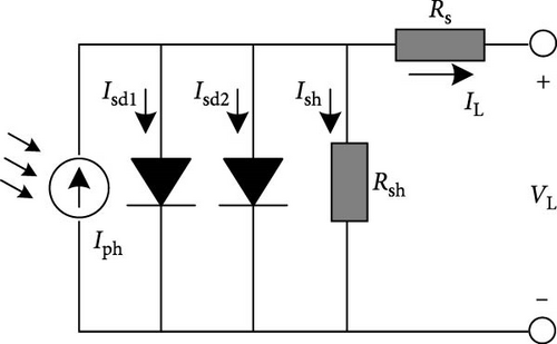
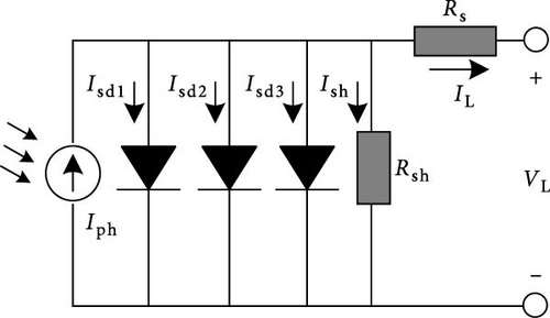
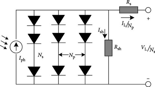
Accurate PV cell models are essential for studying the operation of PV systems. There are four main types of PV parameter identification models: SDM, double diode models (DDM), triple diode models (TDM), and PV module models (PVM). The model and its objective function are described below.

2.1. SDM

The SDM [41] consists mainly of a current source, a diode in parallel with the current source, a series resistor, and a shunt resistor, as shown in Figure 1. The current source depends on its material properties and external environmental factors; the series resistor helps to equalize the current and improve the thermal stability of the PV cell; and the shunt resistor characterizes the shunt leakage current in the semiconductor.

Details are in the caption following the image — **Figure 1**
Open in figure viewer PowerPoint

Equivalent circuit model of SDM.

With the help of Kirchhoff’s current law [42], the relationship between the output current I and diode current I_cd, photocurrent I_ph, and shunt resistance current I_sh can be expressed as follows [43]:

()

According to Shockley’s diode equation, the I_cd and I_sh can be expressed as [43]:

()

where I_sd denotes the saturation current, q stands for the electron charge (q = 1.6021766 × 10⁻¹⁹), n denotes the diode ideality factor, k points to the Boltzmann constant (k = 1.3806503 × 10⁻²³ J/K), T denotes the Kelvin temperature of the cell, V is the output voltage, and R_sh and R_s are the shunt and series resistances, respectively. Combining Equations (2) and (3) into Equation (1), the output current is expressed as [43]:

()

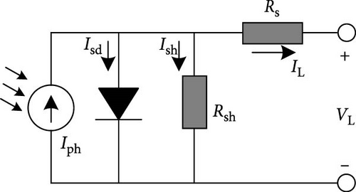
Equation (4) shows that there are {I_ph, I_sd, R_s, R_sh, and n} five unknown parameters that need to be extracted in the SDM.

2.2. DDM

Although the SDM model can be applied to almost all PV cell types, the load current losses in the depletion zone need to be taken into account when in an environment with low irradiation intensity. For this reason, another diode shunt is introduced to simulate the composite currents generated in the circuit, thus forming a DDM, as shown in Figure 2; the output current I is defined as follows [44]:

()

where I_sd1 and I_sd2 stand for the diode’s diffusion and saturation currents and n₁ and n₂ are the ideal factors of the corresponding diodes, respectively. Based on the above analysis, there are seven unknown variables which must be estimated {I_ph, I_sd1, I_sd2, R_S, R_sh, n₁, n₂}.

2.3. TDM

As shown in Figure 3, the three-diode model (TDM) simulates the leakage current in a solar cell by using three diodes; at the same time, the voltage level in the circuit can be adjusted to meet specific requirements or load characteristics. By taking into account more complex factors, it allows the model of TDM to exhibit higher simulation accuracy than SDM and DDM in large-scale industrial silicon cells. The output current I in TDM can be expressed as [45]:

()

where I_sd3 and n₃ denote the saturation current and ideal factor of the newly added diode, and the other variables as well as the parameter definitions are the same as those of the DDM. Nine unknown variables {I_ph, I_sd1, I_sd2, I_sd3, R_s, R_sh, n₁, n₂, n₃} that need to be estimated are required in this model.

2.4. PVM

In production, there is usually a high demand for PV cell output power, and a single PV cell model can no longer meet the actual demand. In order to improve the cell performance and use the cell efficiency, a series of series, parallel, and series-parallel combination of PVM are proposed. A commonly used PVM is shown in Figure 4. The output current I is calculated as follows:

()

where N_s and N_p, respectively, indicate the number of cells connected in series and parallel in the circuit. Since PV component models are usually composed of several identical SDM models connected in series/parallel, there is a need for accurate assessment of five unknown parameters: {I_ph, I_sd, R_s, R_sh, and n}.

2.5. Objective Functions Formulation

Parameter identification in PV cell and module modeling requires the conversion of the established model into a corresponding optimization problem. Typically, in the case of measured current and voltage data, we need to find a set of parameters in the PV model that minimizes the discrepancy between the measured data and the experimentally calculated data. Therefore, the expressions for SDM, DDM, TDM, and PVM are specified as follows:

()

In this study, the root mean square error (RMSE) is used to represent the difference between the simulated and measured current data, and the optimization objective based on the definition of RMSE is expressed as follows:

()

where L expresses the number of the measured data and X expresses the unknown parameter vector to be extracted.

3. RIME Algorithm (RIME)

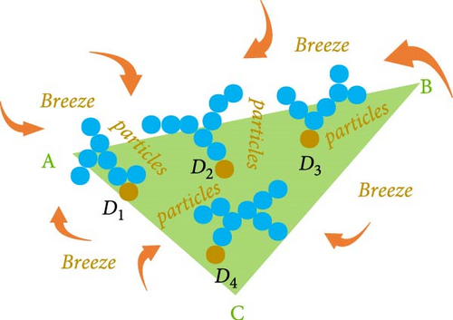
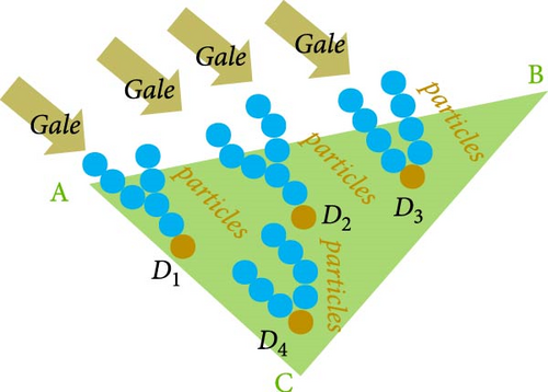
The RIME algorithm mainly completes the search process through the rime initialization phase, soft-rime search phase, hard-rime puncture search phase, and positive greedy selection phase [37]; the soft-rime search phase and hard-rime puncture search phase are shown in Figure 5; and the main principle of RIME is expressed as follows:

3.1. Rime Initialization Phase

The rime population consists of N rime agents, each of which can be represented as a rime particle with D dimensions. Therefore, the rime population x can be represented as follows:

()

where x_ij denotes the position of jth dimension of ith rime agent, N denotes the population size of rime agent, and D represents the dimension of a specific problem.

Similar to most population-based algorithms, the rime population is initialized by completing the initialization process through random search in the initial phase, and then x_ij can be expressed as follows:

()

where Ub_j and Lb_j stand for the upper and lower boundary of jth dimension of the rime population, respectively.

3.2. Soft-Rime Search Phase

The soft-rime search phase is mainly through the simulation of freezing rime with the help of wind force and its own randomness characteristics on the surface of the object free coverage, which ensures that the algorithm has a large search space in the early stage of the iteration. The process of updating the position of rime agent can be expressed as follows:

()

where

stands for the new position of jth dimension of ith rime agent;

stands for the position of jth dimension of the best rime agent at tth iteration in the population; r₁ and cosθ together control the search direction of the rime agent, r₁∈[−1, 1]; θ is defined in the equation; β stands for the environmental factor that models the external environment and ensures the convergence of the rime population, as expressed in the equation; h is the degree of adhesion, which is used to characterize the distance between the best rime agent and a random rime agent, h ∈ [0,1]; r₂ is the random number in [0,1]; and E stands for the attachment coefficient, which affects the coalescence probability of the rime agent and increases gradually as the search proceeds, which is defined as follows:

()

where t stands for the iteration count index and T stands for the number of iterations.

()

where round represents the rounding function, w is used to control the number of segments of the step function, and the default value of w is 5 in the original literature.

3.3. Hard-Rime Puncture Search Phase

The hard-rime puncture search phase mainly considers the mechanism of rime puncture, which produces more crossings between different rime agents in strong wind conditions. Through the principle of rime puncture, the rime agent can exchange more information between agents to ensure that the rime agent can converge to a better position; the formula can be expressed as follows:

()

where

denotes normalized fitness value of

at the tth iteration in the rime population, which is defined as follows:

()

where

denotes origin fitness value of

at the tth iteration.

3.4. Positive Greedy Selection Phase

The greedy selection strategy involves comparing the positions of agents in the population before and after the update. This guarantees that inactive agent positions are replaced with favorable ones, leading to beneficial changes for all agents with respect to their parents each time they are updated. Thus, the utilization of greedy selection guarantees a more favorable evolution of the population with each iteration, as expressed by the following formula:

()

3.5. Flowchart of RIME

The Pseudo-code of the RIME algorithm is given in Algorithm 1.

Algorithm 1: Pseudo-code of RIME.

1. Random initialization of swarm the search space by Equation (14)
2. Evaluate the fitness value of each agent and get the best rime agent in the swarm
3. Whilet < T
4. Calculate the attachment coefficient E by Equation (16)
// Soft-rime search phase
5. Ifr₂ < E
6. Update the agent position of by Equation (15) and Equations (17)–(18)
7. End If
// Hard-rime search phase
8. Calculate the normalized fitness value F^normr () by Equation (20)
9. Ifr₃ < F^normr ()
10. Update the agent position of via Equation (19)
11. End If
// Positive greedy selection phase
12. Comparing the fitness of agents and by Equation (21)
13. t = t + 1
14. End while
15. Output optimal rime agent in the swarm.

4. The ERIME Algorithm

4.1. Motivations

PV model parameter identification is a typical nonlinear optimization problem in the field of optimization, which poses unpredictable challenges to existing methods due to the presence of multiple local minima. In order to solve the PV parameter identification problem, it is usually necessary to propose targeted algorithms or integrate problem-appropriate heuristic strategies into existing methods to satisfy the search requirements at different stages. Therefore, various integration techniques have been developed to effectively solve this problem [10, 46, 47, 47]. However, according to the no free lunch (NFL) theory [48], any one method cannot obtain the optimal solution scheme in all problems; meanwhile, it is found that the RIME method exhibits significant drawbacks in the context of PV parameter identification, particularly manifesting as local stagnation and an imbalance between the exploration and exploitation processes. These deficiencies hinder its ability to efficiently and accurately identify optimal solutions. Local stagnation prevents the algorithm from progressing beyond suboptimal points, while the imbalance between exploration and exploitation limits its capacity to thoroughly search the solution space and effectively refine potential solutions. Consequently, the performance of the RIME method in identifying PV parameters is compromised, necessitating improvements to overcome these limitations. To this end, this paper proposes an ERIME algorithm that combines a modified soft-rime search strategy and a shared information mutation mechanism, which is able to ensure the algorithm’s reasonable balance between exploration and exploitation while avoiding falling into the group local optimum stagnation. The proposed algorithm compensates for the insufficient exploitation of the RIME population by adopting a modified soft-rime search strategy, which effectively improves the solution accuracy. In addition, the shared information mutation mechanism divides the population into two subpopulations for mutation operations; however, unlike the traditional two-population mutation mechanism, there is a common information exchange region in ERIME, which ensures that the algorithm fully utilizes the favorable information in the populations.

4.2. The Modified Soft-Rime Search Strategy

In order to ensure that the algorithm is able to obtain globally optimal solutions in PV parameter identification, it is particularly important to ensure a balanced population exploration and exploitation process. However, in the case of the RIME algorithm, the lack of exploitation capability in the later stages of the search can easily lead to the algorithm not being able to obtain a satisfactory solution for another operator. Therefore, this paper proposes a modified soft-rime search strategy, which introduces a normal distribution function to ensure that RIME is able to search around each agent, and the scope of the search relies on the introduction of the parameter a to ensure the balance between exploration and exploitation, in which in order to ensure that the algorithm is able to ensure the efficiency of the search in the late stage. If β = 0, it indicates that the current agent is stagnant at the current position and cannot perform the performance of the method, while to ensure the randomness of the algorithm, β is randomly searched in a very small range. The modified soft-rime search strategy is expressed as follows:

()

where

stands for the modified position of ith rime agent in jth dimension; the parameter a is defined as follows:

()

where r (0,1) is the random number in the interval [0,1]. G (μ, σ) stands for the normally distributed random number, and its probability density expression is expressed as follows:

()

where X represents a random variable, μ is the position parameter, and σ is the scale parameter.

4.3. The Shared Information Mutation Mechanism

The assurance of diversity during the population search process is beneficial in increasing the chances of the population finding a globally optimal solution. Traditionally, the global population is divided into internal subpopulations according to the rules, and subpopulation evolution can effectively increase the diversity level of the whole population; however, the traditional subpopulation division does not take into account the degree of information exchange of subpopulations in the selection process and cannot make full use of the favorable information of subpopulations. For this reason, this paper designs a shared information variation mechanism to enhance the global search ability of the population, which is easy to fall into the problem of local optimality in the RIME method. Firstly, the current population agents are divided into two subpopulations, A and B, according to their fitness based on their performance; unlike the traditional division, the strategy in this paper makes a common communication space between subpopulations, which ensures that the subpopulations have a full opportunity to communicate with each other. Then, randomly select agents in A and B populations, respectively, for mutation operation, as shown in Figure 6, as follows:

()

where ind1 and ind2 are indexes of rime agent randomly selected from subpopulation A and subpopulation B, respectively. N_sort{1, 2, …, floor(2N/3)} denotes the subpopulation consisting of the first floor(2N/3) individuals after sorting from best to worst according to the fitness of the original population agent. floor denotes the rounding function.

4.4. Framework of Proposed Algorithm

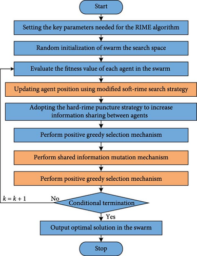
Combining the two proposed effective improvement strategies, this paper proposes an ERIME algorithm, which distinguishes itself from existing optimization algorithms used in power systems by emphasizing balanced exploration and exploitation, achieved through a modified soft-rime search strategy. This approach integrates a normal distribution function to enhance exploration around each agent while preserving the ability to exploit promising areas. Additionally, RIME incorporates a shared information mutation mechanism to facilitate information exchange among agents of different subpopulations, ensuring robust global search capabilities and mitigating the risk of local optima. These features collectively improve the accuracy and efficiency of PV parameter identification. The detailed execution process refers to Algorithm 1, and the flowchart is shown in Figure 7, as follows:

5. Numeral Experimental

5.1. Experiment Settings and Function Details

In order to demonstrate the search performance of the proposed algorithm in numerical optimization problems, in this section, simulation experiments of the method are carried out using the currently popular CEC2022 test suite, as given in Table 2. At the same time, five better-performing control methods are used for comparison to highlight the optimality of the algorithms, including particle swarm algorithm (PSO) [49], multi-verse optimizer (MVO) [50], improved JAYA (IJAYA) [51], whale optimization algorithm (WOA) [52], and RIME [37]. In order to be fair in the comparison of the different algorithms, the search stopping criterion of reaching the maximum number of evaluations of 30,000 is used, with the dimensionality set to 20; the population size is uniformly set to 30; and the algorithms are run independently for 20 runs to statistically analyze the experimental results. Each algorithm was run independently for 20 times to statistically analyze the results. The detailed hyperparameter settings of each algorithm are shown in Table 3.

Table 2. The details of CEC2022 test suite.

Type	No.		Fmin	Range
Unimodal	F₁	Shifted and full rotated Zakharov function	300	[−100, 100]^D

Basic functions	F₂	Shifted and full rotated Rosenbrock’s function	400	[−100, 100]^D
	F₃	Shifted and full rotated expanded Schaffer’s f6 function	600	[−100, 100]^D
	F₄	Shifted and full rotated noncontinuous Rastrigin’s function	800	[−100, 100]^D
	F₅	Shifted and full rotated Levy function	900	[−100, 100]^D

Hybrid functions	F₆	Hybrid Function 1 (N = 3)	1,800	[−100, 100]^D
	F₇	Hybrid Function 2 (N = 6)	2,000	[−100, 100]^D
	F₈	Hybrid Function 3 (N = 5)	2,200	[−100, 100]^D

Composition functions	F₉	Composition Function 1 (N = 5)	2,300	[−100, 100]^D
	F₁₀	Composition Function 2 (N = 4)	2,400	[−100, 100]^D
	F₁₁	Composition Function 3 (N = 5)	2,600	[−100, 100]^D
	F₁₂	Composition Function 4 (N = 6)	2,700	[−100, 100]^D

Table 3. The hyperparameter settings for different methods.

Algorithm	Parameters
PSO	N = 30; personal constant C₁ = 2.0; social constants C₂ = 2.0
MVO	N = 30; probability p = 6.0
WOA	N = 30; constant factor a = 2.0
IJAYA	N = 30
RIME	N = 30; control factor w = 5.0
ERIME	N = 30; control factor w = 5.0, mean μ = 0; standard deviation σ = 1

5.2. Performance Comparison and Analysis of ERIME

Table 4 shows the statistical results of ERIME with the other five methods, mainly consisting of mean and standard deviation. The optimal results of several methods in terms of statistical indicators have been marked in bold. It can be seen that the proposed method excels in overall aspects. In terms of mean values, the proposed method is close to the other popular methods in terms of the F₁, F₃, and F₇ functions, although the results are not optimal. In the other nine test functions, the proposed method achieves the best results in the mean value. This shows that the proposed method is able to maintain a high level of search capability in complex problems. In addition, ERIME is able to achieve the best results in most of the problems, which is a good indication of the stability of the algorithm.

Table 4. The comparison results of ERIME and other methods.

Function	Indictor	ERIME	IJAYA	MVO	PSO	RIME	WOA
F₁	Mean	300.0003	36,129.1195	8,812.176	27,135.84283	7,262.611	15,532.24
F₁	STD	0.000153	8,082.21996	4,773.212	12,579.44259	4,467.763	4,172.2666

F₂	Mean	441.649	474.9469	469.7775	568.3457791	457.8179	533.20058
F₂	STD	18.53256	12.549739	28.31282	92.46921573	32.57485	49.185793

F₃	Mean	618.2604	619.355602	649.6165	616.3373193	624.5321	669.11972
F₃	STD	6.600541	2.29268154	11.572	6.622678286	5.360862	13.988938

F₄	Mean	858.6475	880.79192	915.0768	921.6744587	872.6324	922.8266
F₄	STD	12.57622	20.9927106	35.44931	17.30577899	18.8416	38.572963

F₅	Mean	1,608.96	3,156.01002	3,994.949	2,094.321823	2,166.804	4,213.4535
F₅	STD	769.397	659.159082	1,262.518	738.7364581	502.4909	1,759.4927

F₆	Mean	1,973.927	250,803.076	7,169.645	2,396,482.595	8,350.829	8,4857.413
F₆	STD	82.66188	261,138.554	3,502.739	9,614,460.962	6,599.932	98,492.471

F₇	Mean	2,090.009	2,109.1512	2,227.569	2,082.766193	2,087.344	2,210.3037
F₇	STD	42.25706	16.8285378	115.8984	29.10666718	43.23436	68.54229

F₈	Mean	2,226.06	2,239.96354	2,408.188	2,313.006445	2,301.956	2,273.7696
F₈	STD	5.043835	6.74776693	134.7116	73.55556677	73.51321	61.473868

F₉	Mean	2,480.781	2,483.80188	2,496.115	2,581.323589	2,483.254	2,533.657
F₉	STD	0.000108	1.00645029	26.41138	90.66332607	3.194421	34.362823

F₁₀	Mean	3,095.272	3,906.58809	4,471.547	3,867.797449	3,297.933	4,726.6701
F₁₀	STD	343.5699	1,321.47608	681.421	776.2521077	528.7197	1,302.3993

F₁₁	Mean	2,900.047	3,324.50269	3,016.182	4,719.745011	3,237.2	3,164.8922
F₁₁	STD	79.46173	132.700665	209.2697	771.6220033	1,244.424	190.11188

F₁₂	Mean	2,964.387	2,948.41323	3,236.341	3,030.06564	3,035.993	3,082.7276
F₁₂	STD	21.12499	4.23928791	100.9231	60.85677211	39.94388	96.028653

Friedman rank		1.33	3.67	4.25	4.08	2.83	4.83
Rank		1	3	5	4	2	6

The bold values indicate the best result.

The last two rows of Table 4 give the Friedman test [53] to check whether the proposed method is statistically significant. It can be seen that the proposed method has the best average ranking, with RIME and IJAYA ranking second and third, respectively. Table 5 further gives the results of the Wilcoxon signed-rank test [54] at α = 5%, and the experimental results show that the proposed method is able to continue to outperform its rivals.

Table 5. The Wilcoxon signed-rank results of ERIME with other methods (α = 5%).

Indicator	ERIME vs. IJAYA	ERIME vs. MVO	ERIME vs. PSO	ERIME vs. RIME	ERIME vs. WOA
Win	11	12	10	11	12
Tie	0	0	0	0	0
Lose	1	0	2	1	0
R+	74	78	75	76	78
R-	4	0	3	2	0
P-value	6.04 × 10⁻⁰³	2.22 × 10⁻⁰³	4.74 × 10⁻⁰³	3.70 × 10⁻⁰³	2.22 × 10⁻⁰³
Hypothesis	1	1	1	1	1

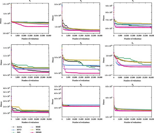
Figure 8 shows the convergence curves of RIME with other methods on the test suite. In F₁, the RIME method converges at a similar speed and accuracy to the control method up to 3,000 times, after which it searches for results with higher accuracy at a faster rate, while the other methods have fallen into local optima. In the convergence graphs of functions F₂–F₆, the proposed method is able to find a more satisfactory solution at the beginning of the search and develop it further. In addition, although the problems of functions F₇–F₉ are more complicated, the proposed method can still maintain high accuracy and search efficiency. In conclusion, it can be shown that the proposed method is an efficient optimization problem-solving tool.

6. Experimental Results and Discussions on PV Problem

To verify the performance of the proposed method on SDM, DDM, TDM, and PVM models. Firstly, the current and voltage datasets of 26 pairs of commercial RTC France PV cell measured under the irradiance of 1,000 W/m² and the temperature of 33°C are selected as the measurement data of SDM, DDM, and TDM to evaluate the unknown parameters of the model [55]. Further, under the irradiance of 1,000 W/m², the current and voltage data collected by Photowatt-PWP 201, single crystal STM6-40/36, and polycrystalline STP6-120/36 module cells at 45, 51, and 55°C were adopted as measurement data to be evaluated with unknown parameters of PVM [56]. In order to be more convincing, the four most popular methods so far, such as PSO, MVO, IJAYA, RIME, and WOA; repairable grey wolf optimization (RGWO) [57]; flexible particle swarm optimization algorithm (FPSO) [36]; and adaptive rat swarm optimization (ARSO) [58], are introduced as control methods for comparison. In order to ensure fair comparison between algorithms, the hyperparameters of each algorithm are consistent with the original literature settings. The maximum number of function evaluations for all methods was set to 40,000, and 20 independent running experiments were performed. The key parameters of different algorithms are set as in the above experiment, and the problem boundary settings of different models are given in Table 6. The performance evaluation index is given by the equation.

Table 6. The lower bound (Lb) and upper bound (Ub) of different parameters for various models.

Parameter	SDM/DDM/TDM		Photowatt-PWP201		STM6-40/36		STP6-120/36
Parameter	Lb	Ub	Lb	Ub	Lb	Ub	Lb	Ub
I_ph (A)	0	1	0	2	0	2	0	8
R_S (Ω)	0	0.5	0	2	0	0.36	0	0.36
R_sh (Ω)	0	100	0	2,000	0	1,000	0	1,500
I_sd, I_sd1, I_sd2, and I_sd3 (μA)	0	1	0	50	0	50	0	50
n, n₁, n₂, and n₃	1	2	1	50	1	60	1	50

()

where IAE and IRE stand for the absolute error and related error of current and PAE stands for the power absolute error.

6.1. Results on SDM, DDM, and TDM

6.1.1. Results on SDM

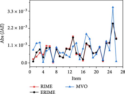
Table 7 shows the optimal parameter results extracted by ERIME with the control methods (PSO, MVO, IJAYA, WOA, and RIME), where the optimal results have been shown in bold. Table 8 further gives the statistical results of the error values of the simulation data and measured data obtained by the proposed method through the optimal parameter results. From the above two tables, it can be seen that the results obtained by the proposed method are the best as compared to the control method, and the proposed method is able to obtain very small absolute error values with respect to most of the measured values.

Table 7. The optimal parameter identification results on SDM.

Algorithm	RMSE	I_ph (A)	I_sd (μA)	R_S (Ω)	R_sh (Ω)	n
PSO	0.001068181	0.760666874	0.398676401	0.03553906	61.52614977	1.502649717
MVO	0.001132318	0.761139577	0.339954315	0.035972223	48.3226622	1.486415638
IJAYA	0.000986586	0.760769337	0.320332355	0.036410397	53.32473299	1.480344347
WOA	0.001453948	0.759885813	0.424449194	0.035188799	86.33212159	1.508908902
RIME	0.000992647	0.760573283	0.322478172	0.036407889	55.70615572	1.48098448
ERIME	0.000986022	0.76077553	0.323020799	0.036377093	53.71852311	1.481183587

The bold values indicate the best result.

Table 8. The comparative results between measured and simulated data on SDM.

Item	Measured data		Simulated current data			Simulated power data
Item	V (V)	I (A)	I (A)	IAE (A)	IRE (%)	P (W)	PAE (W)
1	−0.2057	0.7640	7.64087704E−01	8.77039372E−05	1.14795729E−02	−1.57172841E−01	−1.80406999E−05
2	−0.1291	0.7620	7.62663086E−01	6.63086234E−04	8.70191908E−02	−9.84598044E−02	−8.56044328E−05
3	−0.0588	0.7605	7.61355307E−01	8.55307161E−04	1.12466425E−01	−4.47676921E−02	−5.02920611E−05
4	0.0057	0.7605	7.60153991E−01	−3.46009034E−04	−4.54975719E−02	4.33287775E−03	−1.97225150E−06
5	0.0646	0.7600	7.59055209E−01	−9.44791209E−04	−1.24314633E−01	4.90349665E−02	−6.10335121E−05
6	0.1185	0.7590	7.58042345E−01	−9.57654900E−04	−1.26173241E−01	8.98280179E−02	−1.13482106E−04
7	0.1678	0.7570	7.57091654E−01	9.16538033E−05	1.21075037E−02	1.27039980E−01	1.53795082E−05
8	0.2132	0.7570	7.56141365E−01	−8.58635376E−04	−1.13426073E−01	1.61209339E−01	−1.83061062E−04
9	0.2545	0.7555	7.55086873E−01	−4.13127445E−04	−5.46826533E−02	1.92169609E−01	−1.05140935E−04
10	0.2924	0.7540	7.53663878E−01	−3.36121923E−04	−4.45785044E−02	2.20371318E−01	−9.82820503E−05
11	0.3269	0.7505	7.51390966E−01	8.90966402E−04	1.18716376E−01	2.45629707E−01	2.91256917E−04
12	0.3585	0.7465	7.47353851E−01	8.53851350E−04	1.14380623E−01	2.67926356E−01	3.06105709E−04
13	0.3873	0.7385	7.40117222E−01	1.61722196E−03	2.18987402E−01	2.86647400E−01	6.26350066E−04
14	0.4137	0.7280	7.27382225E−01	−6.17774906E−04	−8.48591905E−02	3.00918027E−01	−2.55573479E−04
15	0.4373	0.7065	7.06972652E−01	4.72651504E−04	6.69004252E−02	3.09159141E−01	2.06690503E−04
16	0.4590	0.6755	6.75280152E−01	−2.19848396E−04	−3.25460246E−02	3.09953590E−01	−1.00910414E−04
17	0.4784	0.6320	6.30758272E−01	−1.24172750E−03	−1.96475871E−01	3.01754758E−01	−5.94042438E−04
18	0.4960	0.5730	5.71928358E−01	−1.07164167E−03	−1.87022980E−01	2.83676466E−01	−5.31534270E−04
19	0.5119	0.4990	4.99607019E−01	6.07018567E−04	1.21647007E−01	2.55748833E−01	3.10732805E−04
20	0.5265	0.4130	4.13648792E−01	6.48791945E−04	1.57092481E−01	2.17786089E−01	3.41588959E−04
21	0.5398	0.3165	3.17510109E−01	1.01010921E−03	3.19149828E−01	1.71391957E−01	5.45256950E−04
22	0.5521	0.2120	2.12154939E−01	1.54938670E−04	7.30842783E−02	1.17130742E−01	8.55416397E−05
23	0.5633	0.1035	1.02251311E−01	−1.24868865E−03	−1.20646247E + 00	5.75981637E−02	−7.03386318E−04
24	0.5736	−0.0100	−8.71754195E−03	1.28245805E−03	−1.28245805E + 01	−5.00038206E−03	7.35617936E−04
25	0.5833	−0.1230	−1.25507413E−01	−2.50741273E−03	2.03854693E + 00	−7.32084738E−02	−1.46257384E−03
26	0.5900	−0.2100	−2.08472326E−01	1.52767392E−03	−7.27463771E−01	−1.22998672E−01	9.01327613E−04

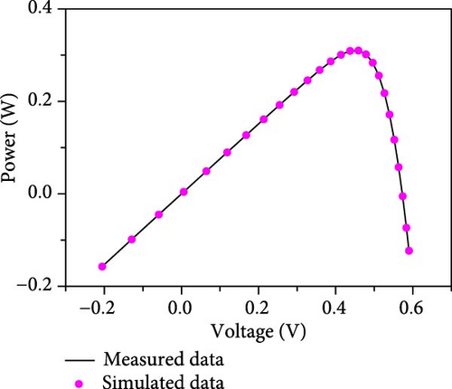
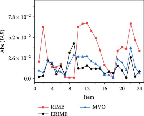
The results of the current–voltage (I–V), power–voltage (P–V) and current error value (IAE) fits are further given in Figures 9(a), 9(b), and 9(c) in conjunction with the measured data. From the figure, it can be seen that the proposed method is able to obtain reliable parameter identification results in the SDM problem.

6.1.2. Results on DDM

The parameter results of the DDM model extracted by ERIME are shown in Table 9. Also, the optimal parameter results of the control methods (PSO, MVO, IJAYA, WOA, and RIME) are listed in the table. It can be seen that the proposed method gives the best RMSE values even if the number of parameters to be determined increases. The simulated current and power data obtained through ERIME results are given in Table 10. By comparing with the real current and power results, it can be seen that the proposed method has very low error values.

Table 9. The optimal parameter identification results on DDM.

Algorithm	RMSE	I_ph (A)	I_sd1 (μA)	R_S (Ω)	R_sh (Ω)	n₁	I_{sd2 (μA)}	n₂
PSO	0.000990127	0.76075025	0.32843973	0.036200774	55.11305065	1.483698232	0.025510287	1.749030543
MVO	0.001697627	0.760805833	0.528696471	0.033735429	67.24729401	1.537531561	0.207947585	1.811797321
IJAYA	0.000986874	0.760820578	0.241969453	0.036581817	55.14230812	1.458574158	0.31125081	1.826206022
WOA	0.00118447	0.759965069	0.071462985	0.035675563	75.72135471	1.687534217	0.359550315	1.495665929
RIME	0.001005833	0.760601256	0.254812457	0.03634022	60.58674374	1.462588269	0.735193716	2
ERIME	0.000983051	0.760780431	0.484418375	0.036585433	54.95105908	1.998129861	0.25901387	1.462542472

The bold values indicate the best result.

Table 10. The comparative results between measured and simulated data on DDM.

Item	Measured data		Simulated current data			Simulated power data
Item	V (V)	I (A)	I (A)	IAE (A)	IRE (%)	P (W)	PAE (W)
1	−0.2057	0.7640	7.64015829E−01	1.58288634E−05	2.07184077E−03	−1.57158056E−01	−3.25599721E−06
2	−0.1291	0.7620	7.62623122E−01	6.23122168E−04	8.17745627E−02	−9.84546451E−02	−8.04450718E−05
3	−0.0588	0.7605	7.61344505E−01	8.44505221E−04	1.11046051E−01	−4.47670569E−02	−4.96569070E−05
4	0.0057	0.7605	7.60169586E−01	−3.30413777E−04	−4.34469134E−02	4.33296664E−03	−1.88335853E−06
5	0.0646	0.7600	7.59093952E−01	−9.06047586E−04	−1.19216788E−01	4.90374693E−02	−5.85306740E−05
6	0.1185	0.7590	7.58100142E−01	−8.99858068E−04	−1.18558375E−01	8.98348668E−02	−1.06633181E−04
7	0.1678	0.7570	7.57162700E−01	1.62699520E−04	2.14926710E−02	1.27051901E−01	2.73009794E−05
8	0.2132	0.7570	7.56217331E−01	−7.82668948E−04	−1.03390878E−01	1.61225535E−01	−1.66865020E−04
9	0.2545	0.7555	7.55156402E−01	−3.43597525E−04	−4.54794871E−02	1.92187304E−01	−8.74455701E−05
10	0.2924	0.7540	7.53713432E−01	−2.86568356E−04	−3.80064133E−02	2.20385807E−01	−8.37925873E−05
11	0.3269	0.7505	7.51407747E−01	9.07747317E−04	1.20952341E−01	2.45635193E−01	2.96742598E−04
12	0.3585	0.7465	7.47329729E−01	8.29729236E−04	1.11149261E−01	2.67917708E−01	2.97457931E−04
13	0.3873	0.7385	7.40054290E−01	1.55428987E−03	2.10465791E−01	2.86623026E−01	6.01976466E−04
14	0.4137	0.7280	7.27294626E−01	−7.05373508E−04	−9.68919654E−02	3.00881787E−01	−2.91813020E−04
15	0.4373	0.7065	7.06885724E−01	3.85723646E−04	5.45964114E−02	3.09121127E−01	1.68676950E−04
16	0.4590	0.6755	6.75219544E−01	−2.80456041E−04	−4.15182889E−02	3.09925771E−01	−1.28729323E−04
17	0.4784	0.6320	6.30738979E−01	−1.26102101E−03	−1.99528640E−01	3.01745528E−01	−6.03272449E−04
18	0.4960	0.5730	5.71949456E−01	−1.05054397E−03	−1.83341007E−01	2.83686930E−01	−5.21069810E−04
19	0.5119	0.4990	4.99653382E−01	6.53381754E−04	1.30938227E−01	2.55772566E−01	3.34466120E−04
20	0.5265	0.4130	4.13694842E−01	6.94842395E−04	1.68242711E−01	2.17810335E−01	3.65834521E−04
21	0.5398	0.3165	3.17535671E−01	1.03567104E−03	3.27226236E−01	1.71405755E−01	5.59055226E−04
22	0.5521	0.2120	2.12147337E−01	1.47336526E−04	6.94983612E−02	1.17126544E−01	8.13444958E−05
23	0.5633	0.1035	1.02214664E−01	−1.28533597E−03	−1.24187050E + 00	5.75775202E−02	−7.24029753E−04
24	0.5736	−0.0100	−8.74637807E−03	1.25362193E−03	−1.25362193E + 01	−5.01692246E−03	7.19077542E−04
25	0.5833	−0.1230	−1.25517899E−01	−2.51789851E−03	2.04707196E + 00	−7.32145902E−02	−1.46869020E−03
26	0.5900	−0.2100	−2.08409158E−01	1.59084188E−03	−7.57543750E−01	−1.22961403E−01	9.38596707E−04

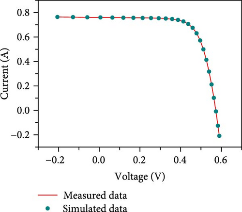
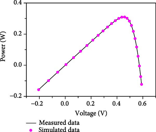
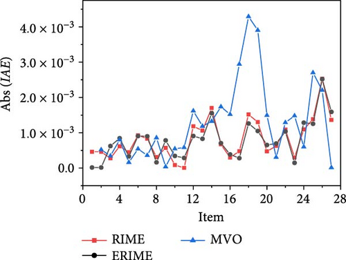
The characteristic curves of I–V,P–V and current error value (IAE) further obtained through ERIME parameter extraction results are given in Figures 10(a), 10(b), and 10(c). It can be noticed that the proposed method is effective in assessing the quality of the cell for the DDM model structure.

6.1.3. Results on TDM

Similarly, the proposed method with the control method is used to extract the TDM model with nine unknown parameters. Table 11 gives the optimal parameter extraction results of different methods for the TDM problem. The error values between the simulated data and the real data obtained by the proposed method are given in Table 12. It is clear to see that the IAE as well as PAE obtained by the proposed method is very low even when more unknown parameters are to be extracted, which proves the robustness of the method.

Table 11. The optimal parameter identification results on TDM.

Algorithm	RMSE	I_ph (A)	I_sd1 (μA)	R_S (Ω)	R_sh (Ω)	n₁	I_{sd2 (μA)}	n₂	I_{sd3 (μA)}	n₃
PSO	0.000994332	0.760760023	0	0.036097921	55.28322567	1	0.344935424	1.487827882	0	2
MVO	0.001887555	0.763125962	0.855898465	0.036765656	35.03862067	1.97118878	0.248176626	1.953639942	0.159859083	1.422754282
IJAYA	0.000992341	0.760784876	0.426237886	0.037061683	58.3033387	1.964276044	0.550783207	1.799127303	0.126555353	1.408181542
WOA	0.001347989	0.75950189	0	0.036869057	74.30746136	1.155647828	0	1.083939433	0.319084001	1.479686995
RIME	0.001118644	0.760074662	0.226941018	0.036756397	72.20923886	1.727060862	0.361026843	1.571126538	0.030996839	1.343175481
ERIME	0.000982601	0.760781489	0.624216927	0.036684854	55.2087035	1.99948144	0.009226936	1.928946253	0.239033778	1.4557175

The bold values indicate the best result.

Table 12. The comparative results between measured and simulated data on TDM.

Item	Measured data		Simulated current data			Simulated power data
Item	V (V)	I (A)	I (A)	IAE (A)	IRE (%)	P (W)	PAE (W)
1	−0.2057	0.7640	7.64000540E−01	5.39715444E−07	7.06433827E−05	−1.57154911E−01	−1.11019467E−07
2	−0.1291	0.7620	7.62614320E−01	6.14320221E−04	8.06194515E−02	−9.84535087E−02	−7.93087405E−05
3	−0.0588	0.7605	7.61341618E−01	8.41617746E−04	1.10666370E−01	−4.47668871E−02	−4.94871235E−05
4	0.0057	0.7605	7.60172012E−01	−3.27988283E−04	−4.31279793E−02	4.33298047E−03	−1.86953321E−06
5	0.0646	0.7600	7.59100938E−01	−8.99061968E−04	−1.18297627E−01	4.90379206E−02	−5.80794032E−05
6	0.1185	0.7590	7.58110657E−01	−8.89342882E−04	−1.17172975E−01	8.98361129E−02	−1.05387131E−04
7	0.1678	0.7570	7.57175201E−01	1.75201495E−04	2.31441869E−02	1.27053999E−01	2.93988109E−05
8	0.2132	0.7570	7.56229547E−01	−7.70453014E−04	−1.01777149E−01	1.61228139E−01	−1.64260583E−04
9	0.2545	0.7555	7.55165329E−01	−3.34671056E−04	−4.42979558E−02	1.92189576E−01	−8.51737838E−05
10	0.2924	0.7540	7.53715721E−01	−2.84278646E−04	−3.77027382E−02	2.20386477E−01	−8.31230760E−05
11	0.3269	0.7505	7.51400840E−01	9.00840186E−04	1.20032004E−01	2.45632935E−01	2.94484657E−04
12	0.3585	0.7465	7.47313207E−01	8.13206707E−04	1.08935929E−01	2.67911785E−01	2.91534604E−04
13	0.3873	0.7385	7.40031485E−01	1.53148470E−03	2.07377752E−01	2.86614194E−01	5.93144024E−04
14	0.4137	0.7280	7.27272658E−01	−7.27341748E−04	−9.99095808E−02	3.00872699E−01	−3.00901281E−04
15	0.4373	0.7065	7.06873890E−01	3.73889820E−04	5.29214183E−02	3.09115952E−01	1.63502018E−04
16	0.4590	0.6755	6.75225050E−01	−2.74950401E−04	−4.07032422E−02	3.09928298E−01	−1.26202234E−04
17	0.4784	0.6320	6.30762346E−01	−1.23765448E−03	−1.95831405E−01	3.01756706E−01	−5.92093902E−04
18	0.4960	0.5730	5.71984046E−01	−1.01595443E−03	−1.77304437E−01	2.83704087E−01	−5.03913395E−04
19	0.5119	0.4990	4.99687815E−01	6.87814959E−04	1.37838669E−01	2.55790192E−01	3.52092478E−04
20	0.5265	0.4130	4.13715243E−01	7.15242761E−04	1.73182267E−01	2.17821075E−01	3.76575314E−04
21	0.5398	0.3165	3.17533746E−01	1.03374613E−03	3.26618049E−01	1.71404716E−01	5.58016158E−04
22	0.5521	0.2120	2.12120499E−01	1.20498587E−04	5.68389561E−02	1.17111727E−01	6.65272699E−05
23	0.5633	0.1035	1.02170071E−01	−1.32992900E−03	−1.28495556E + 00	5.75524010E−02	−7.49149007E−04
24	0.5736	−0.0100	−8.78531060E−03	1.21468940E−03	−1.21468940E + 01	−5.03925416E−03	6.96745838E−04
25	0.5833	−0.1230	−1.25539930E−01	−2.53993048E−03	2.06498413E + 00	−7.32274414E−02	−1.48154145E−03
26	0.5900	−0.2100	−2.08386436E−01	1.61356449E−03	−7.68364042E−01	−1.22947997E−01	9.52003048E−04

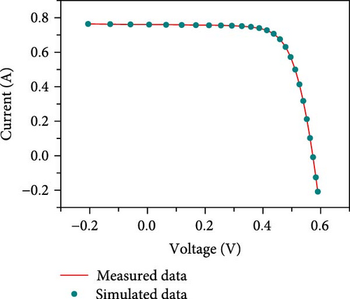
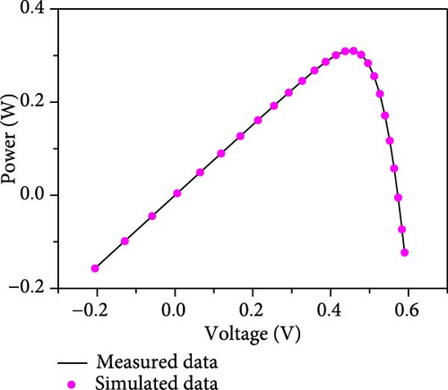
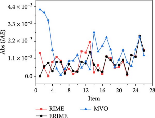
The characteristic curves of current, power versus voltage and current error value (IAE) plotted in conjunction with Table 12 are given in Figures 11(a), 11(b), and 11(c). The high accuracy of the proposed method for parameter extraction for the TDM model is further illustrated.

6.2. Experiments on Different PVM

To demonstrate the practicality of the proposed method, this study evaluates the proposed method in three different PVM model products.

6.2.1. Results on Photowatt-PWP201

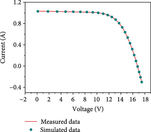
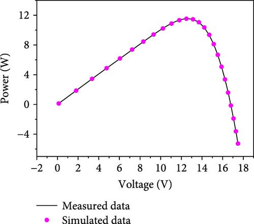
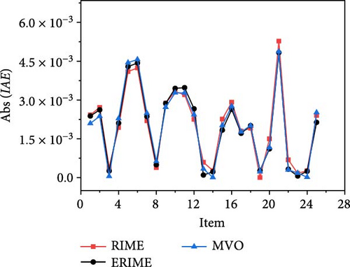
Table 13 presents the optimal parameter statistics for multiple methods in the Photowatt-PWP201 model. Building on the results from Table 13, Table 14 further provides a comparison of the proposed method with other methods using measured data. It is evident that the proposed method outperforms all other methods. Additionally, the statistics of error values show that the current error varies between −4.83282782E−03 and 4.43068116E−03, while the voltage error varies between −7.98581302E−02 and 3.87772777E−02. These small errors indicate that the proposed method achieves the highest accuracy in unknown parameter extraction within PVM models. The robustness of the proposed method is further illustrated by the characteristic curves of I–V and P–V, and IAE, which are plotted in Figures 12(a), 12(b), and 12(c).

Table 13. The optimal parameter identification results on Photowatt-PWP201.

Algorithm	RMSE	I_ph (A)	I_sd (μA)	R_S (Ω)	R_sh (Ω)	n
PSO	0.002445336	1.029847098	3.898829489	1.189410271	1122.847617	49.07897292
MVO	0.002431777	1.030834508	3.395411267	1.204679263	959.6998811	48.5457469
IJAYA	0.002426502	1.030440845	3.493455099	1.200710015	982.4075136	48.65518758
WOA	0.002708903	1.028738172	2.985086984	1.229504732	1189.286689	48.04671727
RIME	0.002440897	1.030520594	3.216021917	1.210457426	954.0354524	48.33772907
ERIME	0.002425075	1.030514298	3.482263117	1.201271005	981.9823871	48.64283508

The bold values indicate the best result.

Table 14. The comparative results between measured and simulated data on Photowatt-PWP201.

Item	Measured data		Simulated current data		Simulated power data
Item	V (V)	I (A)	I (A)	IAE (A)	P (W)	PAE (W)
1	0.1248	1.0315	1.02911916E + 00	−2.38083926E−03	1.28434071E−01	−2.97128740E−04
2	1.8093	1.03	1.02738107E + 00	−2.61892720E−03	1.85884058E + 00	−4.73842499E−03
3	3.3511	1.026	1.02574180E + 00	−2.58203239E−04	3.43736334E + 00	−8.65264875E−04
4	4.7622	1.022	1.02410715E + 00	2.10715480E−03	4.87700309E + 00	1.00346926E−02
5	6.0538	1.018	1.02229180E + 00	4.29180473E−03	6.18875013E + 00	2.59817275E−02
6	7.2364	1.0155	1.01993068E + 00	4.43068116E−03	7.38062638E + 00	3.20621812E−02
7	8.3189	1.014	1.01636311E + 00	2.36310604E−03	8.45502304E + 00	1.96584428E−02
8	9.3097	1.01	1.01049615E + 00	4.96151707E−04	9.40741602E + 00	4.61902355E−03
9	10.2163	1.0035	1.00062897E + 00	−2.87102993E−03	1.02227257E + 01	−2.93313030E−02
10	11.0449	0.988	9.84548379E−01	−3.45162126E−03	1.08742384E + 01	−3.81228116E−02
11	11.8018	0.963	9.59521676E−01	−3.47832379E−03	1.13240829E + 01	−4.10504817E−02
12	12.4929	0.9255	9.22838818E−01	−2.66118202E−03	1.15289331E + 01	−3.32458809E−02
13	13.1231	0.8725	8.72599663E−01	9.96626005E−05	1.14512126E + 01	1.30788227E−03
14	13.6983	0.8075	8.07274263E−01	−2.25736625E−04	1.10582850E + 01	−3.09220801E−03
15	14.2221	0.7265	7.28336478E−01	1.83647769E−03	1.03584742E + 01	2.61185693E−02
16	14.6995	0.6345	6.37138000E−01	2.63799978E−03	9.36561003E + 00	3.87772777E−02
17	15.1346	0.5345	5.36213063E−01	1.71306303E−03	8.11537022E + 00	2.59265238E−02
18	15.5311	0.4275	4.29511325E−01	2.01132493E−03	6.67078334E + 00	3.12380886E−02
19	15.8929	0.3185	3.18774483E−01	2.74482949E−04	5.06625098E + 00	4.36233005E−03
20	16.2229	0.2085	2.07389507E−01	−1.11049303E−03	3.36445923E + 00	−1.80154174E−02
21	16.5241	0.101	9.61671722E−02	−4.83282782E−03	1.58907597E + 00	−7.98581302E−02
22	16.7987	−0.008	−8.32538570E−03	−3.25385697E−04	−1.39855657E−01	−5.46605672E−03
23	17.0499	−0.111	−1.10936482E−01	6.35177170E−05	−1.89145593E + 00	1.08297072E−03
24	17.2793	−0.209	−2.09247265E−01	−2.47265493E−04	−3.61564627E + 00	−4.27257463E−03
25	17.4885	−0.303	−3.00863587E−01	2.13641342E−03	−5.26165283E + 00	3.73626660E−02

6.2.2. Result on STM6-40/36

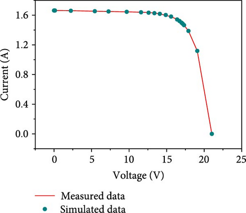
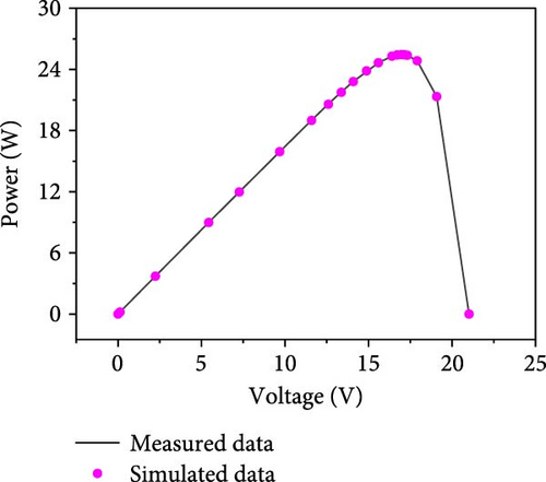
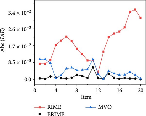
For STM6-40/36 case, the comparison results of the proposed method with the control method are given in Table 15. It can be seen that the proposed method reduces the RMSE values by 0.00160064, 0.003627511, 0.000028539, 0.006867368, and 0.018499327 as compared to PSO, MVO, IJAYA, WOA, and RIME, respectively, which is a good indication of the fact that the proposed method is more efficient than the control method in terms of RMSE values, and it is a good indication of the fact that the proposed method is less expensive than the control method in terms of RMSE value. Table 16 further gives the ratio of the error values of the proposed method for the current and voltage to the measured data, and it can be seen that they are very close to each other for both current and voltage data. Figures 13(a), 13(b), and 13(c) further illustrates the fitting results of the measured and simulated data for the I–V and P–V characteristics (Figures 13(a) and 13(b)), along with the corresponding error statistics shown in Figure 13(c). It is noteworthy that the simulated current and voltage data from the proposed method closely align with the measured data, exhibiting smaller error results. This sufficiently demonstrates that the proposed method effectively enhances the search performance of the algorithm by integrating improved strategies.

Table 15. The optimal parameter identification results on STM6-40/36.

Algorithm	RMSE	I_ph (A)	I_sd (μA)	R_S (Ω)	R_sh (Ω)	n
PSO	0.003330454	1.661447864	5.53805806	0	23.87605311	1.659298281
MVO	0.005357325	1.652871807	7.080456896	0.000329425	710.3947536	1.691191338
IJAYA	0.001758353	1.664420087	1.547190751	0.004666306	15.34698132	1.507564962
WOA	0.008597182	1.646746518	4.757037726	0	886.5880522	1.638288982
RIME	0.020229141	1.67089394	24.405172	0	990.0226787	1.880632472
ERIME	0.001729814	1.663904777	1.738656855	0.004273771	15.92829406	1.520302919

The bold values indicate the best result.

Table 16. The comparative results between measured and simulated data on STM6-40/36.

Item	Measured data		Simulated current data		Simulated power data
Item	V (V)	I (A)	I (A)	IAE (A)	P (W)	PAE (W)
1	0	1.663	1.66345826E + 00	4.58255416E−04	0.00000000E + 00	0.00000000E + 00
2	0.118	1.663	1.66325231E + 00	2.52307134E−04	1.96263772E−01	2.97722418E−05
3	2.237	1.661	1.65955081E + 00	−1.44919403E−03	3.71241515E + 00	−3.24184705E−03
4	5.434	1.653	1.65391470E + 00	9.14696546E−04	8.98737246E + 00	4.97046103E−03
5	7.26	1.65	1.65056591E + 00	5.65911344E−04	1.19831085E + 01	4.10851636E−03
6	9.68	1.645	1.64543060E + 00	4.30602302E−04	1.59277682E + 01	4.16823028E−03
7	11.59	1.64	1.63923353E + 00	−7.66465624E−04	1.89987167E + 01	−8.88333658E−03
8	12.6	1.636	1.63371269E + 00	−2.28730663E−03	2.05847799E + 01	−2.88200635E−02
9	13.37	1.629	1.62728581E + 00	−1.71419453E−03	2.17568112E + 01	−2.29187809E−02
10	14.09	1.619	1.61831357E + 00	−6.86426933E−04	2.28020382E + 01	−9.67175548E−03
11	14.88	1.597	1.60309004E + 00	6.09004222E−03	2.38539798E + 01	9.06198282E−02
12	15.59	1.581	1.58158837E + 00	5.88373650E−04	2.46569627E + 01	9.17274520E−03
13	16.4	1.542	1.54233059E + 00	3.30588167E−04	2.52942216E + 01	5.42164594E−03
14	16.71	1.524	1.52119263E + 00	−2.80736900E−03	2.54191289E + 01	−4.69111359E−02
15	16.98	1.5	1.49919474E + 00	−8.05258487E−04	2.54563267E + 01	−1.36732891E−02
16	17.13	1.485	1.48527527E + 00	2.75267308E−04	2.54427653E + 01	4.71532899E−03
17	17.32	1.465	1.46565424E + 00	6.54239621E−04	2.53851314E + 01	1.13314302E−02
18	17.91	1.388	1.38758937E + 00	−4.10633745E−04	2.48517255E + 01	−7.35445037E−03
19	19.08	1.118	1.11839137E + 00	3.91374448E−04	2.13389074E + 01	7.46742447E−03
20	21.02	0	−2.48104389E−05	−2.48104389E−05	−5.21515426E−04	−5.21515426E−04

6.2.3. Result on STP6-120/36

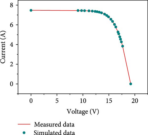
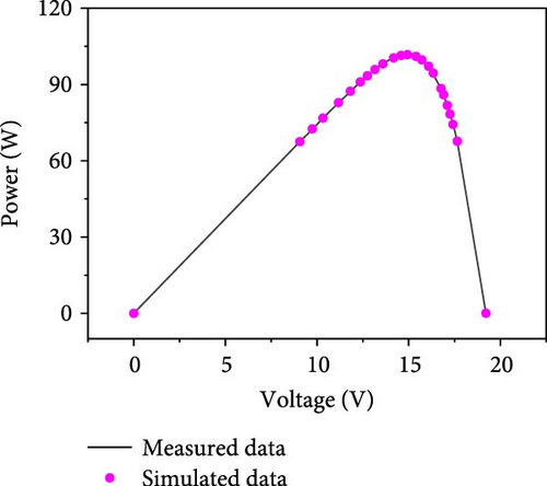
The results of the parameter identification of the proposed method with other control methods in the STP6-120/36 model are shown in Table 17, which mainly consists of five parameters along with the RMSE values. It can be seen from the table that ERIME obtains better RMSE results than other methods. Table 18 further gives the comparison between the simulated test data and the actual measured data obtained by the proposed method, and the results show that the IAE values of the proposed method are between −2.80736900E−03 and 6.09004222E−03, and the PAE values are between −4.69111359E−02 and 9.06198282E−02, and based on the above reported results, it can be concluded that the proposed method is able to identify the PVM model effectively.

Table 17. The optimal parameter identification results on STP6-120/36.

Algorithm	RSME	I_ph (A)	I_sd (μA)	R_S (Ω)	R_sh (Ω)	n
PSO	0.035402678	7.502848591	15.63249687	0.00351853	1,500	1.442259603
MVO	0.019032429	7.473604316	4.128533887	0.004334613	1,129.556374	1.309507916
IJAYA	0.016873239	7.459941061	2.734017349	0.004530463	1,500	1.273353099
WOA	0.043841975	7.495409095	18.73263706	0.003216758	1,440.355312	1.46158395
RIME	0.041089462	7.514991671	22.16233966	0.00329236	1,500	1.481555705
ERIME	0.016600603	7.472529901	2.334995084	0.004594635	22.21993012	1.260103479

The bold values indicate the best result.

Table 18. The comparative results between measured and simulated data on STP6-120/36.

Item	Measured data		Simulated current data		Simulated power data
Item	V (V)	I (A)	I (A)	IAE (A)	P (W)	PAE (W)
1	19.21	0	2.28263097E−03	2.28263097E−03	4.38493409E−02	4.38493409E−02
2	17.65	3.83	3.83334720E + 00	3.34719744E−03	6.76585780E + 01	5.90780349E−02
3	17.41	4.29	4.26733758E + 00	−2.26624167E−02	7.42943473E + 01	−3.94552676E−01
4	17.25	4.56	4.54114855E + 00	−1.88514535E−02	7.83348124E + 01	−3.25187572E−01
5	17.1	4.79	4.78440021E + 00	−5.59978786E−03	8.18132436E + 01	−9.57563724E−02
6	16.9	5.07	5.08557807E + 00	1.55780683E−02	8.59462694E + 01	2.63269355E−01
7	16.76	5.27	5.27482246E + 00	4.82246041E−03	8.84060244E + 01	8.08244364E−02
8	16.34	5.75	5.78259748E + 00	3.25974776E−02	9.44876428E + 01	5.32642784E−01
9	16.08	6	6.04431798E + 00	4.43179788E−02	9.71926331E + 01	7.12633099E−01
10	15.71	6.36	6.34712091E + 00	−1.28790944E−02	9.97132694E + 01	−2.02330573E−01
11	15.39	6.58	6.56654991E + 00	−1.34500908E−02	1.01059203E + 02	−2.06996897E−01
12	14.93	6.83	6.81361105E + 00	−1.63889512E−02	1.01727213E + 02	−2.44687042E−01
13	14.58	6.97	6.95770972E + 00	−1.22902826E−02	1.01443408E + 02	−1.79192321E−01
14	14.17	7.1	7.08757580E + 00	−1.24242037E−02	1.00430949E + 02	−1.76050967E−01
15	13.59	7.23	7.21738487E + 00	−1.26151333E−02	9.80842603E + 01	−1.71439662E−01
16	13.16	7.29	7.28399958E + 00	−6.00042274E−03	9.58574344E + 01	−7.89655633E−02
17	12.74	7.34	7.33134549E + 00	−8.65451049E−03	9.34013415E + 01	−1.10258464E−01
18	12.36	7.37	7.36318321E + 00	−6.81678782E−03	9.10089445E + 01	−8.42554974E−02
19	11.81	7.38	7.39599986E + 00	1.59998557E−02	8.73467583E + 01	1.88958296E−01
20	11.17	7.41	7.42031576E + 00	1.03157604E−02	8.28849270E + 01	1.15227044E−01
21	10.32	7.44	7.43908982E + 00	−9.10179676E−04	7.67714069E + 01	−9.39305426E−03
22	9.74	7.42	7.44676210E + 00	2.67621030E−02	7.25314629E + 01	2.60662884E−01
23	9.06	7.45	7.45254041E + 00	2.54040638E−03	6.75200161E + 01	2.30160818E−02
24	0	7.48	7.47097940E + 00	−9.02060320E−03	0.00000000E + 00	0.00000000E + 00

Figures 14(a), 14(b), and 14(c) presents a detailed comparison of the estimated values of ERIME with the actual measurements. From the simulation results, it can be seen that the simulated current–voltage and simulated power–voltage obtained by the proposed method are in good agreement with the actual characteristic curves, which demonstrates the ability of the proposed RIME method to accurately capture the power generation characteristics of PV cells.

6.3. Statistical Results Analysis

The performance evaluation of the proposed ERIME algorithm needs to be evaluated by multiple computational metrics. Table 19 gives details of the computational metrics, including the optimal value, median, mean, worst value, standard deviation, and (time) average execution time of the algorithms, for each of the algorithms under different PV models for 20 independent runs. Among them, the smaller optimal value indicates the higher accuracy of the algorithm, and the smaller mean and STD (standard deviation) characterize the higher level of the algorithm to avoid premature convergence. From the table, we can see that the proposed method is better than the other eight control methods in terms of optimal value, median, mean, worst value, and standard deviation; specifically, in terms of standard deviation in SDM, the proposed method reduces 1.12E−02, 2.02E−03, 8.84E−05, 1.89E−02, 1.27E−02,1.53E−02,1.17E-02, and 6.72E−04, respectively, compared to PSO, MVO, IJAYA, WOA, RIME, ARSO, FPSO, and RGWO. In terms of average execution time, the proposed method though is similar to the other methods.

Table 19. The statistical results obtained by various methods on different models.

Function	Method	Best	Median	Mean	Worst	STD	Time
SDM	PSO	0.001068181	0.001998167	0.005531128	0.038151316	0.011166373	0.087
	MVO	0.001132318	0.002057314	0.003068542	0.007217234	0.002019791	0.102
	IJAYA	0.000986586	0.000998598	0.001028925	0.001366016	8.84437E−05	0.096
	WOA	0.001453948	0.006687895	0.018043656	0.046856357	0.018912314	0.091
	ARSO	0.01444009	0.023741551	0.028398838	0.054457317	0.012717496	0.039
	FPSO	0.001012725	0.002126272	0.008158853	0.046013568	0.015263371	0.038
	RGWO	0.002939514	0.009149124	0.013172087	0.040511369	0.011740014	0.053
	RIME	0.000992647	0.002079889	0.002101248	0.003551153	0.000671535	0.097
	ERIME	9.86021878E−04	9.86021878E−04	9.86021878E−04	9.86021878E−04	4.00791594E−17	0.104

DDM	PSO	0.000990127	0.002427166	0.009023655	0.03948799	0.014312674	0.103
	MVO	0.001697627	0.003236121	0.003738357	0.008885977	0.001752205	0.109
	IJAYA	0.000986874	0.0010161	0.001062595	0.001338666	0.000101312	0.109
	WOA	0.00118447	0.002122955	0.006957991	0.042112577	0.010158958	0.110
	ARSO	0.004046547	0.021715086	0.021982001	0.042107176	0.011785614	0.051
	FPSO	0.001215071	0.002448049	0.007338198	0.043495207	0.012835419	0.051
	RGWO	0.003966691	0.007197173	0.008835605	0.042122235	0.008189208	0.072
	RIME	0.001005833	0.001823055	0.002010876	0.004040904	0.000985289	0.115
	ERIME	9.83051497E−04	9.84993563E−04	9.85003917E−04	9.87672700E−04	1.25947672E−06	0.117

TDM	PSO	0.000994332	0.002276351	0.017536177	0.191125756	0.042828628	0.137
	MVO	0.001887555	0.002797808	0.003333507	0.00692121	0.001553588	0.137
	IJAYA	0.000992341	0.001013985	0.001096751	0.001398399	0.00013416	0.129
	WOA	0.001347989	0.004153205	0.009189198	0.044536284	0.012012349	0.124
	ARSO	0.007805789	0.024399956	0.025072666	0.034305855	0.005634489	0.058
	FPSO	0.001368654	0.002167688	0.008327167	0.036297802	0.012719265	0.061
	RGWO	0.005409982	0.010472056	0.018219709	0.041970137	0.013738068	0.088
	RIME	0.001118644	0.002441621	0.002494416	0.004491961	0.00094356	0.133
	ERIME	9.82600674E−04	9.85546404E−04	9.88652857E−04	1.03889189E−03	1.20837572E−05	0.142

PV_PWP201	PSO	0.002445336	0.002608134	0.036804184	0.274250778	0.084007926	0.074
	MVO	0.002431777	0.002665561	0.016490241	0.274250823	0.060673253	0.142
	IJAYA	0.002426502	0.002432762	0.00243897	0.002527151	2.16361E-05	0.080
	WOA	0.002708903	0.012038495	0.116728217	0.274352338	0.13314498	0.077
	ARSO	0.013150219	0.027232241	0.02623238	0.040542673	0.008894267	0.038
	FPSO	0.00247552	0.002608134	0.029143791	0.274250778	0.065882268	0.034
	RGWO	0.004488224	0.007757141	0.035192878	0.274292152	0.081860987	0.053
	RIME	0.002440897	0.002606807	0.002953233	0.005063505	0.000665031	0.089
	ERIME	2.42507487E−03	2.42507487E−03	2.42507487E−03	2.42507487E−03	2.34379915E−17	0.082

PV_STM6_40	PSO	0.003330454	0.005360369	0.086701769	0.310757409	0.133212246	0.073
	MVO	0.005357325	0.023471373	0.105507261	0.310757448	0.138048163	0.080
	IJAYA	0.001758353	0.002103419	0.002225532	0.003329793	0.00044539	0.086
	WOA	0.008597182	0.025267461	0.057896963	0.310965197	0.089020092	0.087
	ARSO	0.007265003	0.02259609	0.022655042	0.063728938	0.012868287	0.035
	FPSO	0.003330321	0.004966507	0.111368941	0.310757409	0.150113441	0.032
	RGWO	0.006220049	0.012464276	0.014176619	0.051723576	0.009717092	0.051
	RIME	0.020229141	0.032755934	0.031601786	0.033339326	0.003329882	0.077
	ERIME	1.72981371E−03	1.72981371E−03	1.72981371E−03	1.72981371E−03	3.49060259E−13	0.089

PV_STP6_120	PSO	0.035402678	0.249523985	0.726613588	1.413122041	0.640914017	0.066
	MVO	0.019032429	0.054405107	0.252639044	1.413121505	0.500248446	0.092
	IJAYA	0.016873239	0.017572389	0.01818413	0.024365155	0.002115459	0.076
	WOA	0.043841975	0.430899334	0.621754493	1.715656706	0.530687957	0.077
	ARSO	0.093082339	0.323020844	0.313795587	0.574137574	0.129178508	0.038
	FPSO	0.017315179	0.247968398	0.668896023	1.413122041	0.627840292	0.033
	RGWO	0.058030304	0.094848335	0.306418152	1.413122662	0.480692984	0.053
	RIME	0.041089462	0.055037931	0.053591986	0.055433217	0.003331194	0.080
	ERIME	1.66006031E−02	1.66006031E−02	1.66006037E−02	1.66006100E−02	1.75412134E−09	0.086

The bold values indicate the best result.

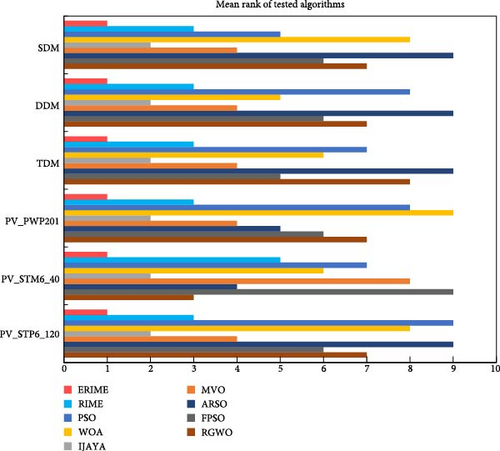
Figure 15 further gives the ranking of the mean values of the different methods on the different tested models; it can be seen that the proposed method has the best ranking among all the six models, followed by the IJAYA method; and the worst overall ranking is the WOA method, which shows the ease with which WOA can fall into a local optimum in solving the PV problem. Therefore, we can conclude that the parameter estimates obtained by the proposed method have a higher accuracy and perform better on average compared to the PV evaluation parameter results obtained by the other eight methods used.

7. Conclusions

In this paper, a boosted RIME algorithm is proposed for extracting the model parameters of SDM, DDM, TDM, and PVM cell models. The effectiveness of the proposed technique is verified by analyzing the proposed method with the control method in terms of results and multiple metrics. The main findings of the work in this paper are as follows:

(1)
Firstly, modified soft-rime search strategy is proposed to enhance the exploitation of the original RIME algorithm, which effectively improves the accuracy of the algorithm; furthermore, a shared information mutation mechanism is proposed to increase the degree of information exchange between different agents of the population throughout the search process, which is conducive to the preservation of the diversity of the population as well as to increase the ability of jumping out of the local optimal point.
(2)
To verify the method search performance, the proposed method is compared with its opponents on the latest test suites. Statistical results show that the proposed method is superior to its peers in terms of convergence speed and solution accuracy and can better balance the exploration and development process. The comparison between the Friedman test and the Wilcoxon signed-rank test also illustrates the advantages of the proposed method.
(3)
The proposed method is employed along with the control method to extract the unknown parameters of different PV cell panels. Simulation results in 20 repetitions of the experiment with RMSE as the optimization objective show that the proposed method is able to produce more accurate results than other methods in SDM, DDM, TDM, and PVM PV cell models. In the statistical analysis of the multiple methods, we can clearly see that the optimal values, mean, and standard deviation obtained by the proposed method are lower than the optimization results obtained by the control method.

Therefore, we finally conclude that the proposed method can effectively improve the level of PV parameter identification and has been proved to be a good method for PV parameter estimation. In future work, we will further consider the modeling of the proposed method under different extreme environmental conditions, such as temperature, light irradiance, and wind speed, and try to improve the adaptability of the proposed method.

Conflicts of Interest

The authors declare no conflict of interest.

Open Research

Data Availability

Data are available on request.

References

1 Yuan X., Su C.-W., Umar M., Shao X., and LOBONŢ O.-R., The race to zero emissions: can renewable energy be the path to carbon neutrality?, Journal of Environmental Management. (2022) 308, https://doi.org/10.1016/j.jenvman.2022.114648, 114648.
10.1016/j.jenvman.2022.114648
CAS PubMed Web of Science® Google Scholar
2 Dinçer F., The analysis on photovoltaic electricity generation status, potential and policies of the leading countries in solar energy, Renewable and Sustainable Energy Reviews. (2011) 15, no. 1, 713–720, https://doi.org/10.1016/j.rser.2010.09.026, 2-s2.0-78149410266.
10.1016/j.rser.2010.09.026
Web of Science® Google Scholar
3 Jordehi A. R., Parameter estimation of solar photovoltaic (PV) cells: a review, Renewable and Sustainable Energy Reviews. (2016) 61, 354–371, https://doi.org/10.1016/j.rser.2016.03.049, 2-s2.0-84964402815.
10.1016/j.rser.2016.03.049
Web of Science® Google Scholar
4 Xiao W., Dunford W. G., and Capel A., A novel modeling method for photovoltaic cells, 2004 IEEE 35th Annual Power Electronics Specialists Conference (IEEE Cat. No.04CH37551), 2004, Aachen, Germany, IEEE, 1950–1956.
Google Scholar
5 Nayak P. K., Mahesh S., Snaith H. J., and Cahen D., Photovoltaic solar cell technologies: analysing the state of the art, Nature Reviews Materials. (2019) 4, no. 4, 269–285, https://doi.org/10.1038/s41578-019-0097-0, 2-s2.0-85063625457.
10.1038/s41578-019-0097-0
CAS Web of Science® Google Scholar
6 Eslami M., Shareef H., Mohamed A., and Khajehzadeh M., A survey on flexible ac transmission systems (facts), Przeglad Elektrotechniczny. (2012) 88, 1–11.
Web of Science® Google Scholar
7 Liu S., Yang Y., Qin H., Liu G., Qu Y., Deng S., Gao Y., Li J., and Guo J., A parameter estimation of photovoltaic models using a boosting flower pollination algorithm, Sensors. (2023) 23, no. 19, https://doi.org/10.3390/s23198324, 8324.
10.3390/s23198324
Web of Science® Google Scholar
8 Yuan S., Ji Y., Chen Y., Liu X., and Zhang W., An improved differential evolution for parameter identification of photovoltaic models, Sustainability. (2023) 15, no. 18, https://doi.org/10.3390/su151813916, 13916.
10.3390/su151813916
CAS Web of Science® Google Scholar
9 Kawamura H., Naka K., Yonekura N., Yamanaka S., Kawamura H., Ohno H., and Naito K., Simulation of I–V characteristics of a PV module with shaded PV cells, Solar Energy Materials and Solar Cells. (2003) 75, no. 3-4, 613–621, https://doi.org/10.1016/S0927-0248(02)00134-4, 2-s2.0-6444245806.
10.1016/S0927-0248(02)00134-4
CAS Web of Science® Google Scholar
10 Oliv D., Aziz M. A. El, and Hassanien A. E., Parameter estimation of photovoltaic cells using an improved chaotic whale optimization algorithm, Applied Energy. (2017) 200, 141–154, https://doi.org/10.1016/j.apenergy.2017.05.029, 2-s2.0-85032814899.
10.1016/j.apenergy.2017.05.029
Web of Science® Google Scholar
11 Xiong G., Zhang J., Shi D., and He Y., Parameter extraction of solar photovoltaic models using an improved whale optimization algorithm, Energy Conversion and Management. (2018) 174, 388–405, https://doi.org/10.1016/j.enconman.2018.08.053, 2-s2.0-85051621834.
10.1016/j.enconman.2018.08.053
Web of Science® Google Scholar
12 Azami H., Malekzadeh M., and Sanei S., A new neural network approach for face recognition based on conjugate gradient algorithms and principal component analysis, Journal of Mathematics and Computer Science. (2013) 6, no. 3, 166–175, https://doi.org/10.22436/jmcs.
10.22436/jmcs.06.03.01
Google Scholar
13 Hejri M., Mokhtari H., Azizian M. R., Ghandhari M., and Soder L., On the parameter extraction of a five-parameter double-diode model of photovoltaic cells and modules, IEEE Journal of Photovoltaics. (2014) 4, no. 3, 915–923, https://doi.org/10.1109/JPHOTOV.2014.2307161, 2-s2.0-84899930825.
10.1109/JPHOTOV.2014.2307161
Web of Science® Google Scholar
14 Wang J., Yang B., Li D., Zeng C., Chen Y., Guo Z., Zhang X., Tan T., Shu H., and Yu T., Photovoltaic cell parameter estimation based on improved equilibrium optimizer algorithm, Energy Conversion and Management. (2021) 236, https://doi.org/10.1016/j.enconman.2021.114051, 114051.
10.1016/j.enconman.2021.114051
Web of Science® Google Scholar
15 Wu Z.-Q., Liu C.-Y., Zhao D.-L., and Wang Y.-Q., Parameter identification of photovoltaic cell model based on improved elephant herding optimization algorithm, Soft Computing. (2023) 27, no. 9, 5797–5811, https://doi.org/10.1007/s00500-023-07819-4.
10.1007/s00500-023-07819-4
Web of Science® Google Scholar
16 Wu Z.-Q., Xie Z.-K., and Liu C.-Y., An improved lion swarm optimization for parameters identification of photovoltaic cell models, Transactions of the Institute of Measurement and Control. (2020) 42, no. 6, 1191–1203, https://doi.org/10.1177/0142331219887844.
10.1177/0142331219887844
Web of Science® Google Scholar
17 Chen H. L., Jiao S., Wang M. J., Heidari A. A., and Zhao X. H., Parameters identification of photovoltaic cells and modules using diversification-enriched harris hawks optimization with chaotic driftse, Journal of Cleaner Production. (2020) 244.
10.1016/j.jclepro.2019.118778
PubMed Web of Science® Google Scholar
18 Yu K., Liang J. J., Qu B. Y., Cheng Z., and Wang H., Multiple learning backtracking search algorithm for estimating parameters of photovoltaic models, Applied Energy. (2018) 226, 408–422, https://doi.org/10.1016/j.apenergy.2018.06.010, 2-s2.0-85048168196.
10.1016/j.apenergy.2018.06.010
Web of Science® Google Scholar
19 Mi X., Liao Z., Li S., and Gu Q., Adaptive teaching-learning-based optimization with experience learning to identify photovoltaic cell parameters, Energy Reports. (2021) 7, 4114–4125, https://doi.org/10.1016/j.egyr.2021.06.097.
10.1016/j.egyr.2021.06.097
Web of Science® Google Scholar
20 Yu S., Chen Z., Heidari A. A., Zhou W., Chen H., and Xiao L., Parameter identification of photovoltaic models using a sine cosine differential gradient based optimizer, IET Renewable Power Generation. (2022) 16, no. 8, 1535–1561, https://doi.org/10.1049/rpg2.12451.
10.1049/rpg2.12451
Web of Science® Google Scholar
21 Oliva D., Ewees A. A., Aziz M. A. E., Hassanien A. E., and Peréz-Cisneros M., A chaotic improved artificial bee colony for parameter estimation of photovoltaic cells, Energies. (2017) 10, no. 7, https://doi.org/10.3390/en10070865, 2-s2.0-85025433973, 865.
10.3390/en10070865
Web of Science® Google Scholar
22 Arandian B., Eslami M., Khalid S. A., Khan B., Sheikh U. U., Akbari E., and Mohammed A. H., An effective optimization algorithm for parameters identification of photovoltaic models, IEEE Access. (2022) 10, 34069–34084, https://doi.org/10.1109/ACCESS.2022.3161467.
10.1109/ACCESS.2022.3161467
Web of Science® Google Scholar
23 Yaghoubi M., Eslami M., Noroozi M., Mohammadi H., Kamari O., and Palani S., Modified salp swarm optimization for parameter estimation of solar pv models, IEEE Access. (2022) 10, 110181–110194, https://doi.org/10.1109/ACCESS.2022.3213746.
10.1109/ACCESS.2022.3213746
Web of Science® Google Scholar
24 Pourmousa N., Ebrahimi S. M., Malekzadeh M., and Alizadeh M., Parameter estimation of photovoltaic cells using improved lozi map based chaotic optimization algorithm, Solar Energy. (2019) 180, 180–191, https://doi.org/10.1016/j.solener.2019.01.026, 2-s2.0-85059894721.
10.1016/j.solener.2019.01.026
Web of Science® Google Scholar
25 Ebrahimi S. M., Malekzadeh M., Alizadeh M., and HosseinNia S. H., Parameter identification of nonlinear system using an improved Lozi map based chaotic optimization algorithm (ILCOA), Evolving Systems. (2021) 12, no. 2, 255–272, https://doi.org/10.1007/s12530-019-09266-9.
10.1007/s12530-019-09266-9
Web of Science® Google Scholar
26 Naeijian M., Rahimnejad A., Ebrahimi S. M., Pourmousa N., and Gadsden S. A., Parameter estimation of PV solar cells and modules using whippy harris hawks optimization algorithm, Energy Reports. (2021) 7, 4047–4063, https://doi.org/10.1016/j.egyr.2021.06.085.
10.1016/j.egyr.2021.06.085
Web of Science® Google Scholar
27 Pourmousa N., Ebrahimi S. M., Malekzadeh M., and Gordillo F., Using a novel optimization algorithm for parameter extraction of photovoltaic cells and modules, The European Physical Journal Plus. (2021) 136, no. 4, https://doi.org/10.1140/epjp/s13360-021-01462-4, 470.
10.1140/epjp/s13360-021-01462-4
CAS Web of Science® Google Scholar
28 Hakmi S. H., Alnami H., Moustafa G., Ginidi A. R., and Shaheen A. M., Modified rime-ice growth optimizer with polynomial differential learning operator for single-and double-diode PV parameter estimation problem, Electronics. (2024) 13, no. 9, https://doi.org/10.3390/electronics13091611, 1611.
10.3390/electronics13091611
CAS Web of Science® Google Scholar
29 Long W., Wu T., Xu M., Tang M., and Cai S., Parameters identification of photovoltaic models by using an enhanced adaptive butterfly optimization algorithm, Energy. (2021) 229, https://doi.org/10.1016/j.energy.2021.120750, 120750.
10.1016/j.energy.2021.120750
Web of Science® Google Scholar
30 Elaziz M. Abd and Oliva D., Parameter estimation of solar cells diode models by an improved opposition-based whale optimization algorithm, Energy Conversion and Management. (2018) 171, 1843–1859, https://doi.org/10.1016/j.enconman.2018.05.062, 2-s2.0-85049594315.
10.1016/j.enconman.2018.05.062
Web of Science® Google Scholar
31 Li S., Gong W., Yan X., Hu C., Bai D., and Wang L., Parameter estimation of photovoltaic models with memetic adaptive differential evolution, Solar Energy. (2019) 190, 465–474, https://doi.org/10.1016/j.solener.2019.08.022, 2-s2.0-85070962390.
10.1016/j.solener.2019.08.022
Web of Science® Google Scholar
32 Sharma A., Sharma A., Dasgotra A., Jately V., Ram M., Rajput S., Averbukh M., and Azzopardi B., Opposition-based tunicate swarm algorithm for parameter optimization of solar cells, IEEE Access. (2021) 9, 125590–125602, https://doi.org/10.1109/ACCESS.2021.3110849.
10.1109/ACCESS.2021.3110849
Web of Science® Google Scholar
33 Ayyarao T. S. L. V. and Kumar P. P., Parameter estimation of solar PV models with a new proposed war strategy optimization algorithm, International Journal of Energy Research. (2022) 46, no. 6, 7215–7238, https://doi.org/10.1002/er.7629.
10.1002/er.7629
Web of Science® Google Scholar
34 Kumar C. and Mary D. M., A novel chaotic-driven tuna swarm optimizer with newton-raphson method for parameter identification of three-diode equivalent circuit model of solar photovoltaic cells/modules, Optik. (2022) 264, https://doi.org/10.1016/j.ijleo.2022.169379, 169379.
10.1016/j.ijleo.2022.169379
Web of Science® Google Scholar
35 Singh A., Sharma A., Rajput S., Bose A., and Hu X., An investigation on hybrid particle swarm optimization algorithms for parameter optimization of PV cells, Electronics. (2022) 11, no. 6, https://doi.org/10.3390/electronics11060909, 909.
10.3390/electronics11060909
CAS Web of Science® Google Scholar
36 Ebrahimi S. M., Salahshour E., Malekzadeh M., and Gordillo F., Parameters identification of PV solar cells and modules using flexible particle swarm optimization algorithm, Energy. (2019) 179, 358–372, https://doi.org/10.1016/j.energy.2019.04.218, 2-s2.0-85065832405.
10.1016/j.energy.2019.04.218
CAS Web of Science® Google Scholar
37 Su H., Zhao D., Heidari A. A., Liu L., Zhang X., Mafarja M., and Chen H., RIME: A physics-based optimization, Neurocomputing. (2023) 532, 183–214, https://doi.org/10.1016/j.neucom.2023.02.010.
10.1016/j.neucom.2023.02.010
Web of Science® Google Scholar
38 Yu X., Qin W., Lin X., Shan Z., Huang L., Shao Q., Wang L., and Chen M., Synergizing the enhanced RIME with fuzzy K-nearest neighbor for diagnose of pulmonary hypertension, Computers in Biology and Medicine. (2023) 165, https://doi.org/10.1016/j.compbiomed.2023.107408, 107408.
10.1016/j.compbiomed.2023.107408
PubMed Web of Science® Google Scholar
39 Zhu W., Fang L., Ye X., Medani M., and Escorcia-Gutierrez J., IDRM: Brain tumor image segmentation with boosted RIME optimization, Computers in Biology and Medicine. (2023) 166, https://doi.org/10.1016/j.compbiomed.2023.107551, 107551.
10.1016/j.compbiomed.2023.107551
PubMed Web of Science® Google Scholar
40 Ismaeel A. A. K., Houssein E. H., Khafaga D. S., Aldakheel E. A., AbdElrazek A. S., and Said M., Performance of osprey optimization algorithm for solving economic load dispatch problem, Mathematics. (2023) 11, no. 19, https://doi.org/10.3390/math11194107, 4107.
10.3390/math11194107
Web of Science® Google Scholar
41 Rhouma M. B. H., Gastli A., Brahim L. B., Touati F., and Benammar M., A simple method for extracting the parameters of the PV cell single-diode model, Renewable Energy. (2017) 113, 885–894, https://doi.org/10.1016/j.renene.2017.06.064, 2-s2.0-85021235187.
10.1016/j.renene.2017.06.064
Web of Science® Google Scholar
42 Labate G. and Matekovits L., Kirchhoff’s current law as local cloaking condition: theory and applications, Electronics Letters. (2016) 52, no. 21, 1728–1751, https://doi.org/10.1049/el.2016.2682, 2-s2.0-84990194985.
10.1049/el.2016.2682
Web of Science® Google Scholar
43 Liang J., Qiao K., Yu K., Ge S., Qu B., Xu R., and Li K., Parameters estimation of solar photovoltaic models via a self-adaptive ensemble-based differential evolution, Solar Energy. (2020) 207, 336–346, https://doi.org/10.1016/j.solener.2020.06.100.
10.1016/j.solener.2020.06.100
Web of Science® Google Scholar
44 Nunes H. G. G., Pombo J. A. N., Bento P. M. R., Mariano S. J. P. S., and Calado M. R. A., Collaborative swarm intelligence to estimate PV parameters, Energy Conversion and Management. (2019) 185, 866–890, https://doi.org/10.1016/j.enconman.2019.02.003, 2-s2.0-85062706322.
10.1016/j.enconman.2019.02.003
Web of Science® Google Scholar
45 Qais M. H., Hasanien H. M., Alghuwainem S., Loo K. H., Elgendy M. A., and Turky R. A., Accurate three-diode model estimation of photovoltaic modules using a novel circle search algorithm, Ain Shams Engineering Journal. (2022) 13, no. 3, https://doi.org/10.1016/j.asej.2022.101824, 101824.
10.1016/j.asej.2022.101824
Web of Science® Google Scholar
46 Liang J., Ge S., Qu B., Yu K., Liu F., Yang H., Wei P., and Li Z., Classified perturbation mutation based particle swarm optimization algorithm for parameters extraction of photovoltaic models, Energy Conversion and Management. (2020) 203, https://doi.org/10.1016/j.enconman.2019.112138, 112138.
10.1016/j.enconman.2019.112138
Web of Science® Google Scholar
47 Kang T., Yao J., Jin M., Yang S., and Duong T., A novel improved cuckoo search algorithm for parameter estimation of photovoltaic (pv) models, Energies. (2018) 11, no. 5, https://doi.org/10.3390/en11051060, 2-s2.0-85047074312, 1060.
10.3390/en11051060
Web of Science® Google Scholar
48 Wolpert D. H. and Macready W. G., No free lunch theorems for optimization, IEEE Transactions on Evolutionary Computation. (1997) 1, no. 1, 67–82, https://doi.org/10.1109/4235.585893, 2-s2.0-0031118203.
10.1109/4235.585893
Google Scholar
49 Eberhart and Yuhui S., Particle swarm optimization: developments, applications and resources, 2001, 81–86.
Google Scholar
50 Mirjalili S., Mirjalili S. M., and Hatamlou A., Multi-verse optimizer: a nature-inspired algorithm for global optimization, Neural Computing and Applications. (2016) 27, no. 2, 495–513, https://doi.org/10.1007/s00521-015-1870-7, 2-s2.0-84955627094.
10.1007/s00521-015-1870-7
Web of Science® Google Scholar
51 Yu K., Liang J. J., Qu B. Y., Chen X., and Wang H., Parameters identification of photovoltaic models using an improved JAYA optimization algorithm, Energy Conversion and Management. (2017) 150, 742–753, https://doi.org/10.1016/j.enconman.2017.08.063, 2-s2.0-85032927573.
10.1016/j.enconman.2017.08.063
Web of Science® Google Scholar
52 Gharehchopogh F. S. and Gholizadeh H., A comprehensive survey: whale optimization algorithm and its applications, Swarm and Evolutionary Computation. (2019) 48, 1–24, https://doi.org/10.1016/j.swevo.2019.03.004, 2-s2.0-85062919203.
10.1016/j.swevo.2019.03.004
Web of Science® Google Scholar
53 Ren Y., Gao K., Fu Y., Sang H., Li D., and Luo Z., A novel Q-learning based variable neighborhood iterative search algorithm for solving disassembly line scheduling problems, Swarm and Evolutionary Computation. (2023) 80, https://doi.org/10.1016/j.swevo.2023.101338, 101338.
10.1016/j.swevo.2023.101338
Web of Science® Google Scholar
54 Wang Z., Chen Y., Ding S., Liang D., and He H., A novel particle swarm optimization algorithm with lévy flight and orthogonal learning, Swarm and Evolutionary Computation. (2022) 75, https://doi.org/10.1016/j.swevo.2022.101207, 101207.
10.1016/j.swevo.2022.101207
Google Scholar
55 Easwarakhanthan T., Bottin J., Bouhouch I., and Boutrit C., Nonlinear minimization algorithm for determining the solar cell parameters with microcomputers, International Journal of Solar Energy. (1986) 4, no. 1, 1–12, https://doi.org/10.1080/01425918608909835, 2-s2.0-84888400237.
10.1080/01425918608909835
CAS Google Scholar
56 Li S., Gu Q., Gong W., and Ning B., An enhanced adaptive differential evolution algorithm for parameter extraction of photovoltaic models, Energy Conversion and Management. (2020) 205, https://doi.org/10.1016/j.enconman.2019.112443, 112443.
10.1016/j.enconman.2019.112443
Web of Science® Google Scholar
57 Ebrahimi S. M., Hasanzadeh S., and Khatibi S., Parameter identification of fuel cell using repairable grey wolf optimization algorithm, Applied Soft Computing. (2023) 147, https://doi.org/10.1016/j.asoc.2023.110791, 110791.
10.1016/j.asoc.2023.110791
Web of Science® Google Scholar
58 Eslami M., Akbari E., Sadr S. T. Seyed, and Ibrahim B. F., A novel hybrid algorithm based on rat swarm optimization and pattern search for parameter extraction of solar photovoltaic models, Energy Science & Engineering. (2022) 10, no. 8, 2689–2713, https://doi.org/10.1002/ese3.1160.
10.1002/ese3.1160
Web of Science® Google Scholar

Citing Literature

All articles

Parameter Identification of Photovoltaic Models by an Enhanced RIME Algorithm

Abstract

1. Introduction

2. PV Problem Formulation

2.1. SDM

2.2. DDM

2.3. TDM

2.4. PVM

2.5. Objective Functions Formulation

3. RIME Algorithm (RIME)

3.1. Rime Initialization Phase

3.2. Soft-Rime Search Phase

3.3. Hard-Rime Puncture Search Phase

3.4. Positive Greedy Selection Phase

3.5. Flowchart of RIME

4. The ERIME Algorithm

4.1. Motivations

4.2. The Modified Soft-Rime Search Strategy

4.3. The Shared Information Mutation Mechanism

4.4. Framework of Proposed Algorithm

5. Numeral Experimental

5.1. Experiment Settings and Function Details

5.2. Performance Comparison and Analysis of ERIME

6. Experimental Results and Discussions on PV Problem

6.1. Results on SDM, DDM, and TDM

6.1.1. Results on SDM

6.1.2. Results on DDM

6.1.3. Results on TDM

6.2. Experiments on Different PVM

6.2.1. Results on Photowatt-PWP201

6.2.2. Result on STM6-40/36

6.2.3. Result on STP6-120/36

6.3. Statistical Results Analysis

7. Conclusions

Conflicts of Interest

Open Research

Data Availability

References

Citing Literature

Figures

References

Related

Information