International Journal of Energy Research

Volume 2024, Issue 1 9557596

Research Article

Open Access

Pump Scheduling Optimization in Urban Water Supply Stations: A Physics-Informed Multiagent Deep Reinforcement Learning Approach

Haixiang Ma

orcid.org/0009-0009-9969-3372

School of Automation and School of Artificial Intelligence , Nanjing University of Posts and Telecommunications , Nanjing , 210023 , China , njupt.edu.cn

Search for more papers by this author

Xuechun Wang,

Xuechun Wang

School of Automation and School of Artificial Intelligence , Nanjing University of Posts and Telecommunications , Nanjing , 210023 , China , njupt.edu.cn

Search for more papers by this author

Dongsheng Wang,

Corresponding Author

Dongsheng Wang

[email protected]

orcid.org/0000-0002-8381-0636

School of Automation and School of Artificial Intelligence , Nanjing University of Posts and Telecommunications , Nanjing , 210023 , China , njupt.edu.cn

Search for more papers by this author

Haixiang Ma,

Haixiang Ma

orcid.org/0009-0009-9969-3372

School of Automation and School of Artificial Intelligence , Nanjing University of Posts and Telecommunications , Nanjing , 210023 , China , njupt.edu.cn

Search for more papers by this author

Xuechun Wang,

Xuechun Wang

School of Automation and School of Artificial Intelligence , Nanjing University of Posts and Telecommunications , Nanjing , 210023 , China , njupt.edu.cn

Search for more papers by this author

Dongsheng Wang,

Corresponding Author

Dongsheng Wang

[email protected]

orcid.org/0000-0002-8381-0636

School of Automation and School of Artificial Intelligence , Nanjing University of Posts and Telecommunications , Nanjing , 210023 , China , njupt.edu.cn

Search for more papers by this author

First published: 19 August 2024

https://doi.org/10.1155/2024/9557596

Citations: 2

Academic Editor: Weixin Guan

Share a link

Email
Wechat
Bluesky

Abstract

In the urban water supply system, a significant proportion of energy consumption is attributed to the water supply pumping station (WSPS). The conventional manual scheduling method employed by water supply enterprises imposes a considerable economic burden. In this paper, we intend to minimize the energy cost of WSPS by dynamically adjusting the combination of pumps and their operational states while considering the pressure difference of the main pipe and switching times of pump group. Achieving this goal is challenging due to the lack of accurate mechanistic models of pumps, uncertainty in environmental parameters, and temporal coupling constraints in the database. Consequently, a WSPS pump scheduling algorithm based on physics-informed long short-term memory (PI-LSTM) surrogate model and multiagent deep deterministic policy gradient (MADDPG) is proposed. The proposed algorithm operates without prior knowledge of an accurate mechanistic model of the pump units. Combining data-driven with the physical laws of fluid mechanics improves the prediction accuracy of the model compared to traditional data-based deep learning models, especially when the amount of data is small. Simulation results based on real-world trajectories show that the proposed algorithm can reduce energy consumption by 13.38% compared with the original scheduling scheme. This study highlights the potential of integrating physics-informed deep learning and reinforcement learning to optimize energy consumption in urban water supply systems.

1. Introduction

Water purification plants are an important part of the city’s infrastructure system. The normal operation of the pumping station is crucial for maintaining the proper functioning of the water treatment facilities in the water purification plant and ensuring a reliable water supply to the town. Water purification plants have a large energy consumption, of which water supply pumping stations (WSPSs) account for a large part [1]. The manual scheduling method lacks scientific theoretical guidance as well as long-term planning, and the irrational method brings unnecessary economic burden to the water plant. Therefore, it is very necessary to improve energy efficiency and reduce energy consumption [2]. While ensuring that the pressure difference of the main pipe and switching times of the pump group are within a safe range, minimizing energy consumption can improve the working efficiency and save the operating cost of the waterwork, which is of great significance to saving urban energy consumption and reducing carbon dioxide emissions [3].

Surrogate models are pivotal for alleviating the computational burden associated with multiquery tasks and are crucial for ensuring the efficient and reliable operation of water supply systems. Surrogate modeling for the pumping stations can be categorized into two principal methodologies: physical modeling and data-driven approaches. Physical modeling involves developing detailed simulations of pump groups or piping networks in water treatment facilities, refined via calibration and parameter identification from operational data to predict operational parameters [4, 5]. However, crafting accurate and controllable physical models for waterwork is particularly challenging. It requires the integration of various complex factors, including the dynamic characteristics of pump units, intricate pipe network layouts, nonlinear fluid mechanics, pump performance curves, mechanical properties, and energy losses. Additionally, the state of maintenance, aging, and consequent changes in the performance of pumps and pipes present significant challenges to the long-term accuracy of these models. The efficacy of this approach is heavily dependent on the specific waterwork environment, which limits its generalizability when applied to diverse waterwork contexts [6]. In contrast, data-driven surrogate models, such as support vector machines [7], radial basis functions [8], and long short-term memory (LSTM) [9], operate akin to black boxes. These models do not require a priori knowledge or insight into the underlying system during the learning process, which facilitates ease of use, particularly for complex systems that are not fully understood. LSTM networks can retain a memory of periodic features in time series data by incorporating gate nodes, leading to more accurate predictions [10]. Their function approximation capabilities exceed those of traditional neural network architectures, which has contributed to their growing popularity in recent years [11]. However, they largely depend on the assumption that sufficient data are available to train deep learning models [12]. Black box models can encounter difficulties when the available dataset lacks coverage for certain process variables, especially those that operate at infrequent points. Collecting extensive datasets is often time-consuming, costly, and challenging, and purely data-driven models may not always conform to physical constraints. In comparison to purely data-based deep learning models, physics-informed deep learning integrates data-driven approaches with physical laws, significantly enhancing the predictive accuracy, generalizability, and physical interpretability of the models. By incorporating system dynamics into its loss function, it can accurately and a priori identify nonlinear systems even with smaller datasets and limited computational power. Recently, physics-informed deep learning models have been applied to chaotic systems [13], nonlinear structures [14, 15], structural responses [16], and wind turbine responses [17]. The successful implementation in these areas has inspired application in fluid mechanics where the flow phenomena can be described by the Navier–Stokes equations [18]. However, their application to waterwork pump scheduling remains unexplored.

In recent years, several approaches have been used to solve the problem of scheduling and operational optimization of pump groups in waterwork. These methods include both rule-based algorithms and optimization techniques, such as genetic optimization algorithms [19], dynamic programming [20, 21], particle swarm optimization [22], metaheuristics [23], and more advanced methods such as reinforcement learning [24, 25] and deep reinforcement learning (DRL) [26, 27]. Rule-based algorithms are straightforward and easy to interpret but often lack the flexibility to adapt to new or changing environments. Optimization techniques such as dynamic programming require an exact mathematical formulation of the problem and are usually unsuitable for dealing with the stochastic nature of real-world systems. Genetic algorithms and particle swarm optimization introduce stochastic search methods that can explore a wider solution space but may converge to suboptimal solutions and require extensive tuning of hyperparameters. DRL has made significant progress in solving complex scheduling and optimization problems. Deep deterministic policy gradient (DDPG) integrates policy gradient and Q-learning techniques to effectively optimize policies in high-dimensional continuous action spaces [28]. Additionally, soft actor-critic (SAC) incorporates an entropy regularization term to balance exploration and exploitation during policy optimization, thereby enhancing policy robustness and convergence speed [29]. In [30], a duel-depth Q network is proposed to train an agent that controls the speed of the pump based on the pressure of the instantaneous node. In [31], knowledge-assisted near-end policy gradient is performed using historical nodal pressure data from waterworks to generate optimal parameter trajectories, accommodating pumping station topology and adapting to time-varying water demand. The above methods use a single agent model to control the pumps, and energy-saving studies for WSPSs have not been carried out. Considering the energy-saving scheduling of fixed-frequency pumps and variable-frequency pumps together, directly using a single agent to control the pump group will lead to a sharp increase in the action space of the agent, resulting in low learning efficiency. While ensuring the safety of water pumps and meeting water supply requirements, it is difficult to effectively save energy consumption. In fact, the water supply pump group of the waterwork contains multiple pumps with different parameters, and the waterwork scheduling requires coordinated control between multiple pumps.

Based on existing research, this paper investigates a new method to minimize the energy consumption of pump group in WSPS. The method considers minimizing the switching times of pump group in a day and reducing the pressure difference of the main pipe in adjacent time periods. The objective is to optimize the scheduling of pump group in WSPSs, controlling the combination of pumps and frequency of variable-frequency pump to minimize energy costs while ensuring that the pressure difference of the main pipe and switching times of pump group remain within safe limits. However, there are several challenges to achieving these goals. Firstly, the dynamic modeling of the system is not sufficiently well defined. Secondly, there are spatiotemporal coupling constraints in the database. Finally, uncertain parameters such as the dynamic environment further complicate the problem. Given these challenges, existing model-based or model-free approaches are not suitable for solving our specific problem. To overcome these obstacles, a Markov game formulation is employed to address the challenge of optimal multipump scheduling in WSPS, utilizing a multiagent system for cooperative management of several pumps to enhance energy efficiency, all the while adhering to constraints regarding the pressure difference of the main pipe and switching times of pump group. Then, a PI-LSTM-based surrogate model is developed to incorporate the laws of fluid mechanics into a LSTM network, which accurately predicts the pressure of the main pipe and energy consumption of the pump group. It is used to provide a simulation environment for agent training, eliminating the need to know the pumps’ precise mechanistic model and specific water demand. Furthermore, a water supply pump group control algorithm based on the surrogate model and multiagent deep reinforcement learning (MADRL) [32] is proposed. Each pump agent learns from the dynamic environment and its own experience while taking into account the presence and potential actions of other pump agents, which facilitates flexible and computable coordination among different agents, thus achieving efficient management of the water supply system. Finally, extensive simulations based on real-world trajectories are performed to evaluate the performance of the proposed algorithm. The simulation results demonstrate the effectiveness and robustness of our approach.

2. Methods

2.1. System Model and Problem Formulation

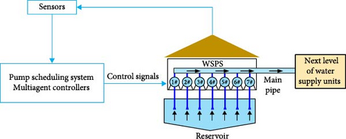
The system model of a waterwork is shown in Figure 1. The WSPS within the waterworks is controlled by a pump scheduling system with multiple fixed-frequency pumps and variable-frequency pumps. We assume that there are N pumps, including M fixed-frequency pumps and N − M variable-frequency pumps. The objective of this paper is to minimize the energy consumption of the WSPS by dynamically adjusting the combination of pumps and their operational states. The scheduling period is assumed to be 1 hr in this paper. To describe the scheduling time more clearly, a day is divided into 24 time slots, i.e., 0 ≤ t ≤ T − 1, where T = 24.

Details are in the caption following the image — **Figure 1**
Open in figure viewer PowerPoint

System model.

2.1.1. Target Constraint

To ensure the production safety and efficient operation of the waterwork, this paper introduces three key constraints: an upper limit on the pressure difference of the main pipe, an upper limit on the switching times of pump group per day, and a range of operating frequencies for the variable-frequency pumps.

Firstly, it is vital that the pressure difference of the main pipe is maintained below a safe upper limit, as excessive pressure difference can lead to pipe rupture accidents, which in turn affects the stability and safety of the water supply system. It is constrained as

(1)

where p^max is the maximum pressure difference allowed and p_t−1, p_t denote the main pipe pressure at neighboring time slot.

Secondly, limiting the switching times of pump group per day helps reduce mechanical wear and energy waste caused by frequent start-stops, thereby extending the pumps’ lifespan and lowering energy costs. It is constrained as

(2)

where v^max is the number of acceptable safe switching of the water supply pump group in a day,

is the number of switching at time slot t, and K_t = [k_1,t, …, k_N,t] is the switching state vector of the pump group at time slot t.

Finally, the operating frequency of the variable-frequency pumps should be controlled within an appropriate range to ensure efficient pump operation and to avoid energy efficiency degradation or equipment damage. It is constrained as

(3)

where

is the minimum operating frequency of the ith variable-frequency pump and

is the maximum operating frequency of the ith variable-frequency pump.

2.1.2. Energy Minimization Problem

The focus of this paper is to minimize the total energy consumption of the WSPS, which is affected by the operational status of the pump group. Then, the expected energy consumption minimization problem is defined as

(4)

where Φ_t is the energy consumption of the water supply pump group at time slot t, E is the expectation operator, s_t is the environmental state of the scheduling system at time slot t, and a_t is the behavior decision of the water supply pump group at time slot t.

However, solving the problem directly has significant challenges. Firstly, high dimensionality and complexity are a major obstacle. Since the optimization problem considers multiple pumps, each of which may have different operating states at different time slots, the state space and decision space are unusually large. This not only increases the computational burden but also makes it more difficult to find the global optimal solution. Then, the uncertainty of the dynamic environment further increases the solution difficulty. Key environmental parameters may change over time, and these changes are often difficult to predict accurately, which means that the solution needs to be able to adapt to possible changes to maintain its effectiveness and robustness.

Given these challenges, transforming the problem into a Markov game provides an efficient solution path. In the Markov game, the pump system is considered as a multiagent system, where each pump is an agent that interacts with each other in a given environment with the common goal of minimizing the overall energy consumption.

2.1.3. Problem Reformulation

Markov game is a multiagent extension of Markov’s decision-making process. Specifically, Markov games can be defined by a series of states, behaviors, state transfer functions, and reward functions. In the Markov game, each agent maximizes its expected return (i.e., the expected value of the cumulative discount reward) based on its current state and choice of its behavior. In this study, each agent i is designated as a pump controller, with the environment encompassing everything interacting with the agents. The objective for each agent is to maximize the cumulative discount rewards received in the future from state s_t and action a_t. Then, the state, action, and reward function in the Markov game are designed.

(1) State. Energy consumption of WSPS is related to p_t, q_t, v_t, k_i,t and f_i,t, with all state components being time-dependent, linked to time slot t. The local observed state of the agent is expressed by o_i,t. Due to the limited availability of local observation information pertaining to the state, the state of each fixed-frequency pump agent can be designed as follows, s_i,t = o_i,t = (p_t, q_t, v_t, k_i,t), 1 ≤ i ≤ M, while the state of each variable-frequency pump agent can be designed as follows, s_i,t = o_i,t = (p_t, q_t, v_t, k_i,t, f_i,t), M < i ≤ N, where p_t is the pressure of the main pipe at time slot t, q_t is the water supply flow at time slot t, v_t is the number of switching at time slot t, k_i,t(1 ≤ i ≤ N) is each pump’s switch condition at time slot t, and f_i,t(M < i ≤ N) is the operating frequency of the ith variable-frequency pump at time slot t.

(2) Action. The behavior at time slot t is denoted by a_t, a_t = (a_1,t, …, a_M,t, a_M+1,t, …, a_N,t). For fixed-frequency pump agents, a_i,t = m_i,t, 1 ≤ i ≤ M, and for variable-frequency pump agents, a_i,t = {m_i,t, Δf_i,t}, M < i ≤ N, where m_i,t ∈ {0, 1}, 1 ≤ i ≤ N denotes the switching action of each agent at time slot t, m_i,t = 0 denotes that the ith pump is switched off at time slot t, m_i,t = 1 denotes that the ith pump is switched on at time slot denotes the frequency change of the ith variable-frequency pump at time slot t.

(3) Reward function. Upon the transition of the environmental state from s_t−1 to s_t due to the collective action a_t−1, the environment yields a reward r_t, r_t = (r_i,t, …, r_N,t). Our objective is to minimize the total energy consumption of WSPS while adhering to constraints concerning the pressure difference of the main pipe and the switching times of pump group. Therefore, the reward function is developed to include penalties for energy consumption, pressure difference of the main pipe, and pump switching at time slot t.

(1) The penalty associated with WSPS energy consumption Φ_t is defined as follows:

(5)

(2) The penalty for violation of the pressure difference of the main pipe is defined as follows:

(6)

(3) The penalty for switching pump i at time slot t is defined as follows:

(7)

(4) The penalty for violating the switching times of pump group per day is defined as follows:

(8)

Therefore, the reward function of each agent is as follows:

(9)

Among them, α₁ is the important factor of the penalty caused by the violation of the safety limit of pressure difference relative to the energy consumption penalty cost, α₂ is the important factor of the penalty caused by switching pumps relative to the energy consumption penalty cost, and α₃ is the important factor of the penalty caused by the violation of the safety range of the switching times relative to the energy consumption penalty cost.

To promote the efficient training of agents, the specific values of these weight coefficients were fine-tuned through experiments and expert opinions to find the optimal balance. In practice, their values should be chosen so that α1C_2,t, α2C_3,t, and α3C_4,t are comparable to C_1,t. Therefore, in this study, α1 = 0.03, α2 = 0.94, and α3 = 3.76.

2.2. Water Supply Pump Group Control Algorithm

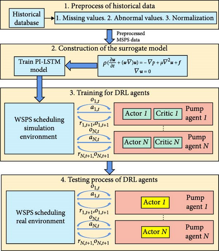
To solve the Markov game in Section 2.1.3, a pump scheduling algorithm for WSPSs based on surrogate model and MADDPG is designed. Employing PI-LSTM as a surrogate model provides a virtual training environment for DRL agents [33]. It obviates the need for direct interaction between multiagent systems and the actual WSPS environment, thereby reducing exploration costs and mitigating associated safety concerns [34]. The framework of the proposed pump scheduling algorithm is shown in Figure 2.

2.2.1. Surrogate Model

Empirical physical models typically cover only common pump combinations [3], whereas multiagent reinforcement learning requires the exploration of novel pump combinations to derive optimization strategies independent of prior experience. To address this need, deep learning-based surrogate models can efficiently simulate the operation state under different pump group configurations to quickly provide an accurate simulation environment for training reinforcement learning agents. Accurate prediction of energy consumption and the main pipe pressure is very important for planning the reliable and effective implementation of WSPS scheduling, so we established a PI-LSTM model to specialize in time series data. The model takes the data related to the state behavior of the pump group of the waterwork at the beginning of the time slot as the input and then outputs the energy consumption Φ_t+1 and the main pipe pressure p_t+1 at the end of the time slot t.

(1) The LSTM cell

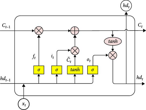
LSTM neural network is comprised of a memory unit and a gating unit, primarily achieving information preservation and control through three gates: the input gate, forget gate, and output gate. The working principle of the neural network t moment is shown in Figure 3.

(2) Fluid mechanics equation

In the context of fluid mechanics within pipe networks, the fundamental equations governing the flow of an incompressible fluid like water are the Navier–Stokes equations and the continuity equation. These equations provide the mathematical framework necessary to describe the motion of fluid particles and are essential for modeling the fluid mechanics in a variety of engineering applications, including water distribution systems.

(i)
Navier–Stokes equation

The Navier–Stokes equations represent the conservation of momentum for fluid flow and can be written for an incompressible fluid as follows:

(10)

where u is the fluid velocity vector field, ρ is the fluid density, p is the pressure field, μ is the kinematic viscosity, and f represents forces per unit mass.

(ii)
Continuity equation

The continuity equation reflects the conservation of mass within a flow and for an incompressible fluid is expressed as follows:

(11)

The Navier–Stokes and continuity equations are central to modeling fluid flow and pressure in pipes, and integrating them into the LSTM model can enhance its predictive accuracy.

(3) The PI-LSTM Model

The structure of the proposed PI-LSTM model is shown in Figure 4. This model is designed to integrate the core principles of fluid mechanics with the predictive capabilities of machine learning. The construction of the model adheres to empirical data as well as established physical laws, thereby enhancing the reliability and accuracy of its predictions.

The loss function is critical for training neural networks. It calculates the deviation between the predicted and actual data to guide the optimization algorithm to adjust the network weights and biases of the network to minimize the loss [35]. It is typically composed of two main parts: the data loss L_data and the physical constraint loss L_phy. Here is how each of these components is defined.

The data loss quantifies the discrepancy between the PI-LSTM model’s predictions and the observed data. This component of the loss function ensures that the model learns to fit the empirical data accurately. It is typically computed as a norm of the difference between the predicted outputs y^′ and the actual outputs y over the training dataset. It is defined as follows:

(12)

where N is the number of data points in the training set, y_i is the actual value of the ith data point, and

is the predicted value for the ith data point.

The physical constraint loss is what distinguishes a PI-LSTM model from a conventional LSTM model. This part of the loss function measures how well the model’s predictions adhere to the underlying physical laws governing the system. The physical constraint loss is formulated based on the residuals of the governing equations evaluated at the model’s predictions. It is defined as follows:

(13)

where λ_i represents the weights of each equation.

Then, the augmented loss function L can be expressed as follows:

(14)

where λ_phy is a weighting factor that adjusts the importance of the physical loss terms relative to the data loss.

The loss function is related to the mean square error term and the system dynamics. Most neural network models only use the mean square error as their loss function. This is the basic difference between other neural networks and physical information neural networks [36].

The scheduling surrogate model of the water supply pump group is constructed as follows:

(15)

(16)

where u_t = (p_t, q_t, a_t) and L_t,1, L_t,2 are PI-LSTM model trained using real historical running data and M is the length of the input data. Calculate the loss from the predicted data with the real end-of-time slot data and update the network parameters. Thus, the surrogate model of waterwork is obtained.

2.2.2. Training Process of the Proposed Algorithm

To train DRL agents effectively, the MADDPG algorithm is adopted [37]. The algorithm aims to enhance the actor-critic framework and the DDPG algorithm by incorporating a centralized training and decentralized execution paradigm. This approach enables the algorithm to tackle intricate multiagent environments, where traditional single-agent reinforcement learning techniques fall short [38, 39].

The framework of MADDPG algorithm is shown in Figure 5, where agents can be identified and each agent consists of one actor network, one critic network, one target actor network, and one target critic network. The actor network and target actor network have the same network architecture, while the critic network and target critic network have the same network architecture.

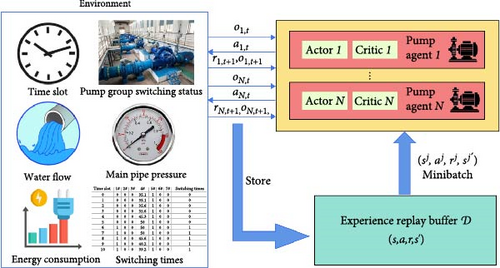
In the MADDPG algorithm environment, there are N agents. For the ith agent, the current state is s_i, the next state is , and the reward is r_i. Each agent has its own action strategy μ_i, policy parameter θ_i, and action a_i, . For all the agents, we define the state set is s = (s₁, …, s_N), the reward set is r = (r₁, …, r_N), the action set is a = (a₁, …, a_N), the action strategy set is μ = (μ₁, …, μ_N), and the policy parameter set is . The centralized action-value function of each agent is denoted as , which combines the states and actions of all agents.

In the decision-making process, all the agents interact with the environment and generate and store data in their own experience replay buffer . For the ith agent, the array stores in the experience replay buffer. When updating the network, groups of data are randomly taken from each agent’s experience replay buffer of each agent and then spliced to obtain new experience (s, a, r, s‘), which is used for training the network.

When training the critic network, the loss function L(θ_i) of the critic network is as follows:

(17)

where yⁱ is the target Q value and it is calculated as

(18)

where i is the sequence number of the agent, j is the sequence number of the sample, γ is the discounted factor,

is the output of the critic-target network,

is the strategy of actor-target network, and θ is the policy parameter of actor-target network. Algorithm training is carried out with the goal of maximizing the reward value while minimizing the L(θ_i) function [40].

The training of the policy network aims to find the optimal solution for the network’s parameters. The algorithm employs stochastic gradient ascent (SGA) to update the policy network parameters [41]. The formula of the actor network update gradient is

(19)

Algorithm 1 is the pseudocode of MADDPG algorithm for WSPS scheduling.

Algorithm 1: Multiagent deep deterministic policy gradient algorithm for N agents.

Initialize: the actor’s evaluation and critic’s target networks for each pump agent
01:for episode = 1 to M do
02: Initialize a radon process for action exploration
03: Receive initial state s
04: for t = 1 to max-episode-length do
05: for each pump agent i, select action w.r.t. the current policy and exploration
06: Execute actions a(t) = (a₁(t), …, a_N(t)) and observe reward r and new state s^′
07: Store (s, a, r, s^′) in replay buffer
08: s←s^′
09: for agent i = 1 to N do
10: Sample a random minibatch of samples (s^j, a^j, r^j, s^′j) from
11: Set
12: Update critic by minimizing the loss
13: Update actor using the sampled policy gradient:
14: end for
15: Update target network parameters for each agent i:
16: end for
17:end for

2.2.3. Testing Process of the Proposed Algorithm

After finishing the training process of the algorithm, the obtained actor networks can be adopted for practical pump scheduling. To be specific, in each time slot t, each pump controller observes the state o_i,t and takes action a_i,t ~ π_θ(⋅|o_i,t) in parallel. Then, all actions are executed. At the end of time slot t, new state o_i,t is observed by pump controller i. The above decision process repeats until the end of slot H_test. Based on the above description, it can be inferred that the proposed algorithm can support real-time decision based on the current system state. Since just the forward propagation of deep neural networks is involved, the proposed algorithm has low computational complexity. Algorithm 2 is the proposed test code.

Algorithm 2: The proposed MADDPG-based WSPS scheduling algorithm.

Input: The weights of the actor network, i.e., θ
Output: Action a_t
1 All agents receive initial local observation o₁ = (o_1,1, ⋅⋅⋅o_N+1)
2 for t = 1, 2, · · ·, H_test do
Each agent i selects its action a_i,t in parallel according to the learned policy π_θ(⋅|o_i,t) at the beginning of slot t
4 Each agent i takes action a_i,t in parallel, which affects the operation of the control system
5 Each agent i receives new observation o_i,t+1 at the end of slot t
6 end

3. Results and Discussion

In simulations, real-world waterwork operation data related to the Baiyangwan Waterwork in Suzhou City, China, during November 1, 2020, and April 30, 2021, are used. Surrogate model uses 80% of the data as a training set and 20% as a test set. All DRL agents are trained using the data during November 1, 2020, and February 28, 2021, while the remaining data are used for performance testing.

3.1. Performance of Surrogate Model

The efficacy of surrogate model in predicting key operational parameters of WSPS systems is critical for optimizing energy consumption and maintaining system integrity. To compare the performance of two predictive models, the selected evaluation metrics are mean absolute error (MAE), mean absolute percentage error (MAPE), and coefficient of determination (R²). Here are their definitions:

(20)

(21)

(22)

where y_i is the actual value,

is the predicted value,

is the mean of the actual values, and n is the number of observations.

Figure 6(a) shows the comparison of energy consumption prediction for a week, and Figure 6(b) shows the comparison of stress prediction for a week. To assess the generalizability of the PI-LSTM model, especially in the case of limited data availability, we halved the data for the experiment, and Figure 6(c) shows the comparison of pressure prediction for a week in that case. As can be seen in Figure 6(a), both models can capture the general trend and major fluctuations in actual energy consumption better. Although the predicted values of the PI-LSTM model are closer to the actual values than those of the LSTM at some points, especially during the peak energy consumption period, in general, the predictive performances of the two models are very similar. The result suggests that, although the PI-LSTM model incorporates fluid mechanics laws, the contribution of this information to the enhancement of energy consumption prediction accuracy is marginal. In this case, the standard LSTM model already captures the key features of the energy consumption of the WSPS better, and the additional physical information does not significantly improve the prediction. As can be seen in Figure 6(b), both models effectively track the general trend of actual pressure. The PI-LSTM model generally exhibits a tighter fit, while the LSTM predictions show larger deviations at certain points, particularly during instances of pressure fluctuation. It shows that the PI-LSTM model, which introduces the laws of fluid mechanics as constraints in the framework and takes into account the movement of fluid and pressure distribution in the pipe, is able to capture the intrinsic laws of pressure changes more accurately compared to LSTM. These physical laws provide additional prior knowledge that helps the model better predict complex pressure dynamics. The standard LSTM model, on the other hand, mainly relies on the laws learned from historical data and lacks the consideration of the underlying physical processes, and the prediction is not accurate enough when facing complex pressure dynamics. As can be seen in Figure 6(c), the PI-LSTM model is still able to generate pressure predictions that are very close to the actual values, despite the fact that the training data is reduced by half. In contrast, the performance of the LSTM model is significantly degraded, with large deviations of the predictions from the actual pressure at more time points. The PI-LSTM model maintains a high predictive accuracy even with less data due to the fluid mechanics equations offering a priori constraints on pressure dynamics, acting as a physics-driven regularization term that allows the model to follow physical laws in making predictions, instead of solely relying on data-driven learning. The standard LSTM model, which is heavily data-dependent, struggles to sufficiently learn key features of pressure dynamics with limited data, resulting in a significant drop in predictive performance. This underscores that pure data-driven learning is not robust when data are scarce, whereas the PI-LSTM model, which integrates physical laws, exhibits stronger generalization capabilities.

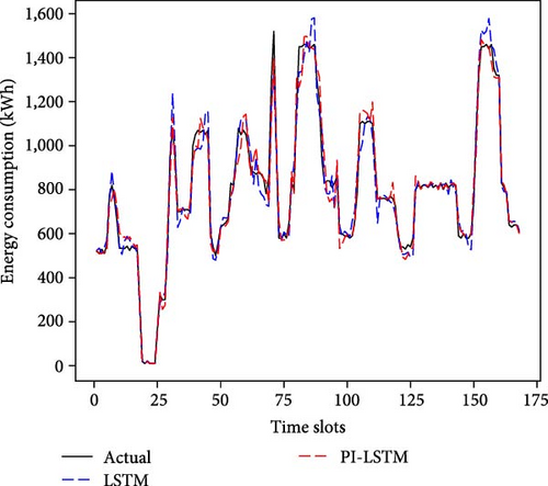
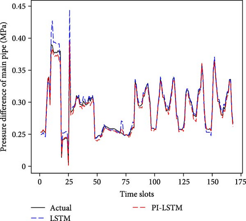
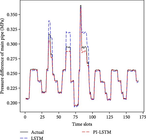
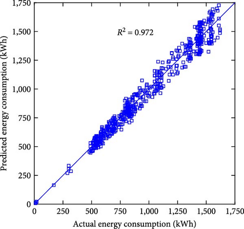
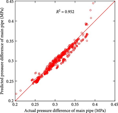
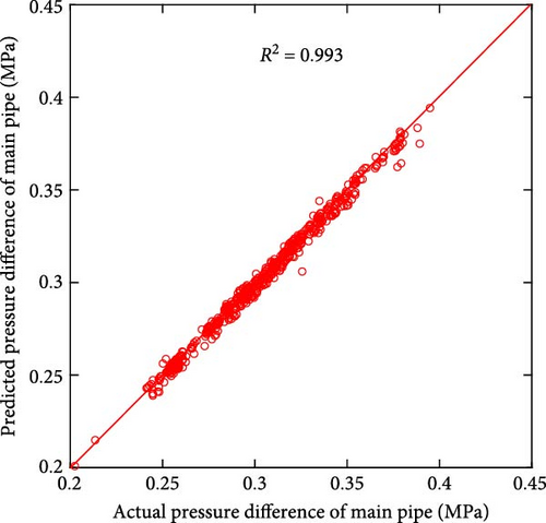
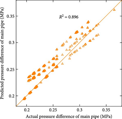
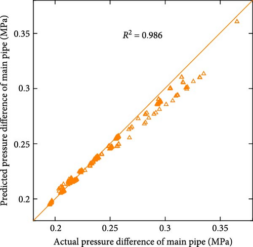
Figure 7 shows the scatter plot of the actual and predicted values of the two models, and Table 1 shows the comparison of the performance error metrics of the two models. Figures 7(a) and 7(b) demonstrate the relationship between the actual and predicted energy consumption for the entire test set for both models. The R² values of the two models are 0.972 and 0.971, respectively, indicating that there is a strong correlation between the predicted and actual values, and both models can effectively capture potential energy consumption patterns. When examining the error metrics, the MAE and MAPE of LSTM are 50.101 kWh and 5.180%, respectively, while those of PI-LSTM are 49.733 kWh and 5.097%. This similarity in performance suggests that PI-LSTM does not have a substantial advantage over LSTM in predicting energy consumption due to the predominance of factors other than fluid mechanics affecting energy consumption patterns. Figures 7(c) and 7(d) demonstrate the relationship between the actual pressure and the predicted pressure for the entire test set of the two models. The R² value of PI-LSTM is 0.993, which is better than 0.952 of LSTM. In terms of error metrics, the MAE of PI-LSTM is 0.003 MPa, which is lower than the 0.006 MPa of LSTM. The MAPE of PI-LSTM is 0.832%, which is significantly lower than 2.069% of LSTM. These show that the PI-LSTM model is significantly more accurate, and the improved accuracy can be attributed to its integration of fluid mechanics constraints. Figures 7(e) and 7(f) demonstrate the relationship between the actual pressure and the predicted pressure for the entire test set of the two models when the data are halved. The PI-LSTM still maintains a high R² of 0.986, while the LSTM decreases to 0.896. The MAE of PI-LSTM is 0.003 MPa, which is lower than the 0.009 MPa of LSTM. The MAPE of PI-LSTM is 1.184%, which is a less significant increase compared to when there is sufficient data, while the MAPE of LSTM is 3.536%, which is a significant increase. These indicate that even with limited data, the PI-LSTM model maintains predictive reliability and accuracy, highlighting its robustness and generalization ability. In contrast, the predictive ability of the LSTM model is greatly reduced, highlighting the limitations of purely data-driven approaches in the presence of insufficient data.

Table 1. Comparative performance metrics of the two models.

Metric	Energy consumption		Pressure		Pressure (data halved)
Metric	LSTM	PI-LSTM	LSTM	PI-LSTM	LSTM	PI-LSTM
MAE	50.101	49.733	0.006	0.003	0.009	0.003
MAPE (%)	5.180	5.097	2.069	0.832	3.536	1.184

A comparative analysis of the performance of the LSTM model and the PI-LSTM model reveals significant advantages of incorporating the laws of physics into a machine learning framework. The higher prediction accuracy of PI-LSTM is attributed to its ability to account for the principles of fluid mechanics that are critical to the operation of WSPS. The LSTM model, though effective in capturing the general patterns, is not sufficiently accurate, which may lead to suboptimal scheduling decisions that can increase operational costs or system instability.

3.2. Performance of the Proposed Algorithm

The specific network parameter design is shown in Table 2. Other main simulation parameters are given as follows: N = 7, M = 5, p^max = 0.08MPa, v^max = 4/day, f^min = 35Hz, f^max = 50Hz, and H_test = 1440h. 1#, 2#, 3#, 5#, and 6# are fixed-frequency pumps, and 4# and 7# are variable-frequency pumps.

Table 2. The neural network and training parameter settings.

Parameter	Value
Neurons of hidden layers for critic networks	128
Learning rate of critic network	0.002
Neurons of hidden layers for actor networks	128
Learning rate of critic network	0.002
Minibatch	120
Buffer size	192,000
Discount factor	0.95
Episodes	40,000

To evaluate the performance of the proposed algorithm, three performance metrics including average energy consumption per slot (AEC in kWh), average switching times of pump group in a day (AST in times/day), and average pressure violation per slot (APV in MPa) are defined as follows:

(23)

(24)

(25)

3.2.1. Algorithm Convergence Process

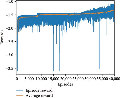
Figure 8 shows the convergence process of the proposed reinforcement learning algorithm over a series of episodes. It can be seen that the curve of episode reward gradually increases and then becomes more and more stable. However, due to the existence of the exploration process and uncertain parameters, the episode reward curve still fluctuates within a narrow gap. It suggests that the algorithm is successfully optimizing its policy toward maximizing rewards. To provide a clearer visualization of the algorithm’s convergence, we present an average reward curve computed over the past 400 episodes. The average reward curve displays an initial increase followed by a stable pattern, indicating that the algorithm’s learning is stabilizing and converging towards a steady and optimized policy.

3.2.2. Algorithm Effectiveness

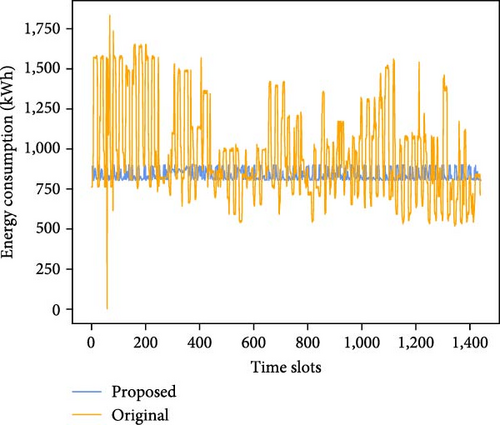
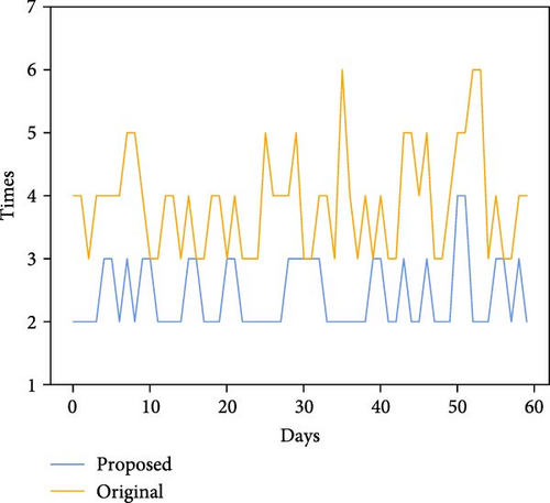
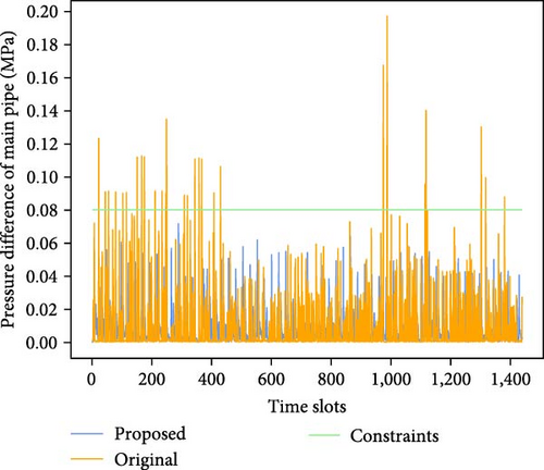
Figure 9 demonstrates the comparison of energy consumption, the pressure difference of the main pipe, and switching times of pump group for the original scheme and the proposed scheme. Table 3 shows the performance comparison for two schemes. From Figure 9(a), it can be seen that the energy consumption of the proposed algorithm is much stable and significantly lower than that of the original scheme, which exhibits substantial fluctuations. From Figure 9(b), it can be seen that the switching times of the proposed scheme are overall much lower than the original. From Figure 9(c), it can be seen that the proposed scheme does not exhibit any pressure difference limit violations, whereas the original scheme experiences multiple occurrences. Manual scheduling relies on experience and heuristic rules, making it difficult to account for various complex factors. In some cases, it exhibited lower energy consumption. To ensure sufficient water supply, waterworks often increase the number of pumps running and crank up the operating frequency of variable-frequency pumps. This results in frequent switching of pumps on and off, leading to frequent large fluctuations in energy consumption and pressure. Although this irrational scheduling scheme can guarantee water supply, it causes substantial energy waste and increases the risk of accidents. The method proposed in this paper focuses on long-term energy optimization, better ensuring the long-term safe and stable operation of the pump system in water plants.

Table 3. Performance comparisons under different schemes.

Schemes	AEC	AST	APV
Original	967.5	3.883	2.1e-3
Proposed	838.1	2.417	0

The average energy consumption per time slot of the original scheme is 967.5 kWh, while the optimized average energy consumption per time slot is 838.1 kWh, which saves 13.38% of the electrical energy. Under dynamic operating conditions, each pump’s energy efficiency varies. The proposed algorithm can flexibly select the most energy-efficient pump combination based on different operating conditions, thereby achieving lower energy consumption. By reasonably planning the pump combination and variable-frequency pump operation frequency, it can minimize the unnecessary pump starts and stops, so that the switching times is greatly reduced from the original average of 3.883 per day to 2.417, a reduction of 37.77%. Fewer switching times of pump group and smaller frequency adjustments of variable-frequency pumps also resulted in reduced fluctuations in energy consumption, which remained in the 800–900 kWh range overall. In contrast, manual scheduling schemes struggle with long-term planning and perform excessive unnecessary switching operations, increasing energy consumption. Specifically, in MADRL algorithm, each pump is considered an agent. Through continuous interaction and game-playing among agents, the globally optimal scheduling strategy is sought. In this process, each pump agent learns and adjusts its behavior strategy based on its own state and environmental feedback to maximize the long-term reward of the entire water supply system. Through distributed learning and collaboration of multiple agents, the algorithm can effectively cope with the complexity, uncertainty, and dynamic changes of the water supply system, which traditional manual scheduling methods cannot effectively address. The learning framework of the algorithm ensures that, over time, the agents become more skilled at maintaining the optimal operating state consistent with the energy-saving objective. In addition, the original scheme had 28 pressure difference transgressions with an average of 0.0021 MPa per time slot, while the proposed algorithm did not have a single transgression. This indicates that the proposed algorithm successfully keeps the pressure variations within safe limits and reduces the potential risks associated with pressure difference overruns.

To present the specific scheduling plan of the proposed algorithm in more detail, Figure 10 shows the scheduling comparison charts of the two schemes for 3 consecutive days, and Figure 11 shows the operation of the variable-frequency pumps.

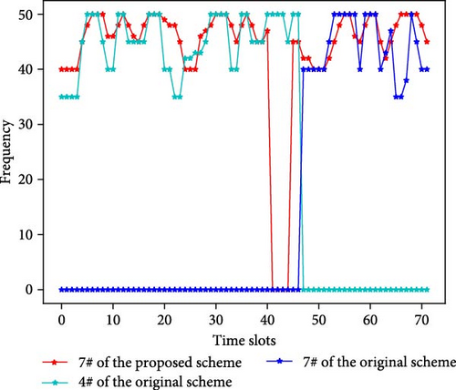
From Figure 10, it can be seen that the switching times of pump group in the original scheme are 14, while the proposed scheme is 7. During this period, the AEC of the original scheme is 973.5 kWh, while the proposed scheme is only 835.8 kWh. As can be seen in Figure 11, the frequency variation range of the variable-frequency pump of the proposed scheme is small in adjacent time slots, while the frequency variation of the original scheme is large, which is not conducive to the protection of the pumps. The proposed scheme is mainly operated by two or three pumps. To be specific, during the daytime and early evening, it is mainly operated by two fixed-frequency pumps and one variable-frequency pump, with the variable-frequency pump running at the highest frequency during the morning, midmorning, and evening peaks and lowering it at other times. During late night and early morning, it is mainly operated by one fixed-frequency pump and one variable-frequency pump, and the variable-frequency pump maintains a lower operating frequency. Over a longer period, the working pumps are more fixed. The frequent switching of the original scheme is unreasonable. There is a situation where four pumps are working at the same time. The working pumps are not fixed.

The frequent switching in the original scheme is due to the lack of comprehensive consideration of various factors and the absence of long-term planning, which resulted in only passive switching to cope with fluctuating demand, leading to energy inefficiency and wear and tear on the pump units. In contrast, the proposed scheme maintains a relatively stable number of pumps throughout the time period, with only minor adjustments when necessary. This shows that the proposed scheme minimizes unnecessary pump switching and improves the reliability and efficiency of the water supply system.

4. Conclusion

This study addresses the complex problem of optimizing energy-saving scheduling in a WSPS with multiple pumps while ensuring compliance with constraints related to the pressure difference of the main pipe and switching times of pump group. The optimization problem is challenging due to parameter uncertainty, temporal coupling constraints, and the lack of an explicit mechanistic model for the pumps. Therefore, the problem is reformulated as a cooperative Markov game. To deal with Markov games, an innovative PI-LSTM surrogate model is developed for training agents, and a WSPS scheduling algorithm based on the surrogate model and MADDPG is proposed. PI-LSTM provides a physical information-driven improvement of the LSTM architecture by incorporating the knowledge of fluid mechanics, which enables it to predict the pressure variations more accurately in the main pipe, especially when there is fewer data. Moreover, the algorithm does not require prior knowledge of the pumps, making it easier to implement in different water plants. Future research could consider integrating more physical laws that are directly related to energy consumption, such as the laws of thermodynamics and electricity, to further improve the performance of the model in energy consumption prediction. In addition, exploring the impact of combining these physical laws with different deep learning models on MADRL could be a valuable direction. Compared with the original scheduling scheme, the proposed algorithm provides a more flexible combination of pumps and achieves the best energy-saving effect, which can reduce energy consumption by 13.38%. This study demonstrates the great potential of multiagent reinforcement learning in the optimal scheduling of water supply systems, which provides important insights for further improving urban water supply management.

Abbreviations

WSPS:: Water supply pumping station
LSTM:: Long short-term memory
PI-LSTM:: Physics-informed long short-term memory
MADDPG:: Multiagent deep deterministic policy gradient
DRL:: Deep reinforcement learning
MADRL:: Multiagent deep reinforcement learning
DDPG:: Deep deterministic policy gradient
SAC:: Soft actor-critic
MAPE:: Mean absolute percentage error
MAE:: Mean absolute error
R²:: Coefficient of determination
AEC:: Average energy consumption
AST:: Average switching times
APV:: Average pressure violation.

Conflicts of Interest

The authors declare that they have no known competing financial interests or personal relationships that could have appeared to influence the work reported in this paper.

Authors’ Contributions

Haixiang Ma contributed to the methodology and wrote, reviewed, and edited the manuscript. Xuechun Wang revised and edited the manuscript. Dongsheng Wang contributed to the conceptualization and methodology.

Acknowledgments

This work was supported by the National Natural Science Foundation of China (grant no. 52170001).

Open Research

Data Availability

The data used to support the findings of this study are available from the corresponding author upon request.

References

1 Lam K. L., Kenway S. J., and Lant P. A., Energy use for water provision in cities, Journal of Cleaner Production. (2017) 143, 699–709, https://doi.org/10.1016/j.jclepro.2016.12.056, 2-s2.0-85008323992.
10.1016/j.jclepro.2016.12.056
Web of Science® Google Scholar
2 Guan W., Guo Y., and Yu G., Carbon materials for solar water evaporation and desalination, Small. (2021) 17, no. 48, https://doi.org/10.1002/smll.202007176, 2007176.
10.1002/smll.202007176
CAS PubMed Web of Science® Google Scholar
3 Wang D., Zhang P., Ma H., Li Z., Xu S., and Tan C., Intelligent collaborative optimal scheduling for water intake-supply pump groups in drinking water treatment plants, International Journal of Energy Research. (2024) 2024, 14, https://doi.org/10.1155/2024/7800284, 7800284.
10.1155/2024/7800284
Web of Science® Google Scholar
4 Olszewski P., Genetic optimization and experimental verification of complex parallel pumping station with centrifugal pumps, Applied Energy. (2016) 178, 527–539, https://doi.org/10.1016/j.apenergy.2016.06.084, 2-s2.0-84979917454.
10.1016/j.apenergy.2016.06.084
Web of Science® Google Scholar
5 Paez D., Suribabu C. R., and Filion Y., Method for extended period simulation of water distribution networks with pressure driven demands, Water Resources Management. (2018) 32, no. 8, 2837–2846, https://doi.org/10.1007/s11269-018-1961-1, 2-s2.0-85044044417.
10.1007/s11269-018-1961-1
Web of Science® Google Scholar
6 Yin W., Fan Z., Tangdamrongsub N., Hu L., and Zhang M., Comparison of physical and data-driven models to forecast groundwater level changes with the inclusion of GRACE—a case study over the state of Victoria, Australia, Journal of Hydrology. (2021) 602, https://doi.org/10.1016/j.jhydrol.2021.126735, 126735.
10.1016/j.jhydrol.2021.126735
Web of Science® Google Scholar
7 Ławryńczuk M., Modelling and predictive control of a neutralisation reactor using sparse support vector machine Wiener models, Neurocomputing. (2016) 205, 311–328, https://doi.org/10.1016/j.neucom.2016.03.066, 2-s2.0-84969581367.
10.1016/j.neucom.2016.03.066
Web of Science® Google Scholar
8 Balla K. M., Jensen T. N., Bendtsen J. D., and Kallesøe C. S., Model predictive control using linearized radial basis function neural models for water distribution networks, 2019 IEEE Conference on Control Technology and Applications (CCTA), 2019, IEEE.
Google Scholar
9 Schwedersky B. B., Flesch R. C. C., and Dangui H. A. S., Practical nonlinear model predictive control algorithm for long short-term memory networks, IFAC-PapersOnLine. (2019) 52, no. 1, 468–473, https://doi.org/10.1016/j.ifacol.2019.06.106, 2-s2.0-85070544361.
10.1016/j.ifacol.2019.06.106
Google Scholar
10 Firouzjaee J. T. and Khalilian P., The interpretability of LSTM models for predicting oil company stocks: impact of correlated features, International Journal of Energy Research. (2024) 2024, 18, https://doi.org/10.1155/2024/5526692, 5526692.
10.1155/2024/5526692
Web of Science® Google Scholar
11 Hart R. G., Griffis E. J., Patil O. S., and Dixon W. E., Lyapunov-based physics-informed long short-term memory (lstm) neural network-based adaptive control, IEEE Control Systems Letters. (2023) .
Google Scholar
12 Zhang R., Liu Y., and Sun H., Physics-guided convolutional neural network (PhyCNN) for data-driven seismic response modeling, Engineering Structures. (2020) 215, https://doi.org/10.1016/j.engstruct.2020.110704, 110704.
10.1016/j.engstruct.2020.110704
Web of Science® Google Scholar
13 Özalp E., Margazoglou G., and Magri L., Physics-informed long short-term memory for forecasting and reconstruction of chaos, International Conference on Computational Science, 2023, Springer.
Google Scholar
14 Zhang R., Liu Y., and Sun H., Physics-informed multi-LSTM networks for metamodeling of nonlinear structures, Computer Methods in Applied Mechanics and Engineering. (2020) 369, https://doi.org/10.1016/j.cma.2020.113226, 113226.
10.1016/j.cma.2020.113226
Web of Science® Google Scholar
15 Zarzycki K. and Ławryńczuk M., Long short-term memory neural networks for modeling dynamical processes and predictive control: a hybrid physics-informed approach, Sensors. (2023) 23, no. 21, https://doi.org/10.3390/s23218898, 8898.
10.3390/s23218898
Web of Science® Google Scholar
16 Liu F., Li J., and Wang L., Pi-Lstm: physics-informed long short-term memory network for structural response modeling, Engineering Structures. (2023) 292, https://doi.org/10.1016/j.engstruct.2023.116500, 116500.
10.1016/j.engstruct.2023.116500
Web of Science® Google Scholar
17 Li X. and Zhang W., Physics-informed deep learning model in wind turbine response prediction, Renewable Energy. (2022) 185, 932–944, https://doi.org/10.1016/j.renene.2021.12.058.
10.1016/j.renene.2021.12.058
Web of Science® Google Scholar
18 Cai S., Mao Z., Wang Z., Yin M., and Karniadakis G. E., Physics-informed neural networks (pinns) for fluid mechanics: a review, Acta Mechanica Sinica. (2021) 37, no. 12, 1727–1738, https://doi.org/10.1007/s10409-021-01148-1.
10.1007/s10409-021-01148-1
Web of Science® Google Scholar
19 Zhang X., Wang D., Jiang F., Lin T., and Xiang H., An optimal regulation method for parallel water-intake pump group of drinking water treatment process, IEEE Access. (2020) 8, 82797–82803.
10.1109/ACCESS.2020.2991895
Web of Science® Google Scholar
20 Chen W., Tao T., Zhou A., Zhang L., Liao L., Wu X., Yang K., Li C., Zhang T. C., and Li Z., Genetic optimization toward operation of water intake-supply pump stations system, Journal of Cleaner Production. (2021) 279, https://doi.org/10.1016/j.jclepro.2020.123573, 123573.
10.1016/j.jclepro.2020.123573
Web of Science® Google Scholar
21 Ramos H. M., Costa L. H. M., and Gonçalves F. V., Energy efficiency in water supply systems: ga for pump schedule optimization and ann for hybrid energy prediction, Water Supply System Analysis-Selected Topics. (2012) .
Google Scholar
22 Maier H. R., Simpson A. R., Zecchin A. C., Foong W. K., Phang K. Y., Seah H. Y., and Tan C. L., Ant colony optimization for design of water distribution systems, Journal of Water Resources Planning and Management. (2003) 129, no. 3, 200–209.
10.1061/(ASCE)0733-9496(2003)129:3(200)
Web of Science® Google Scholar
23 Patel V. K. and Raja B. D., Comparative performance of recent advanced optimization algorithms for minimum energy requirement solutions in water pump switching network, Archives of Computational Methods in Engineering. (2021) 28, no. 3, 1545–1559, https://doi.org/10.1007/s11831-020-09429-x.
10.1007/s11831-020-09429-x
Web of Science® Google Scholar
24 Shyalika C., Silva T., and Karunananda A., Reinforcement learning in dynamic task scheduling: a review, SN Computer Science. (2020) 1, no. 6, https://doi.org/10.1007/s42979-020-00326-5, 306.
10.1007/s42979-020-00326-5
Google Scholar
25 Nian R., Liu J., and Huang B., A review on reinforcement learning: introduction and applications in industrial process control, Computers & Chemical Engineering. (2020) 139, https://doi.org/10.1016/j.compchemeng.2020.106886, 106886.
10.1016/j.compchemeng.2020.106886
CAS Web of Science® Google Scholar
26 Du W. and Ding S., A survey on multi-agent deep reinforcement learning: from the perspective of challenges and applications, Artificial Intelligence Review. (2021) 54, no. 5, 3215–3238, https://doi.org/10.1007/s10462-020-09938-y.
10.1007/s10462-020-09938-y
Web of Science® Google Scholar
27 Hu C., Wang Q., Gong W., and Yan X., Multi-objective deep reinforcement learning for emergency scheduling in a water distribution network, Memetic Computing. (2022) 14, no. 2, 211–223, https://doi.org/10.1007/s12293-022-00366-9.
10.1007/s12293-022-00366-9
Web of Science® Google Scholar
28 Yu L., Xie W., Di X., Zou Y., Zhang D., Sun Z., Zhang L., Zhang Y., and Jiang T., Deep reinforcement learning for smart home energy management, IEEE Internet of Things Journal. (2019) 7, no. 4, 2751–2762, https://doi.org/10.1109/JIoT.6488907.
10.1109/JIOT.2019.2957289
Web of Science® Google Scholar
29 Haarnoja T., Zhou A., Hartikainen K., Tucker G., Ha S., Tan J., Kumar V., Zhu H., Gupta A., Abbeel P., and Levine S., Soft Actor-Critic Algorithms and Applications, 2018, arXiv preprint arXiv: 1812.05905.
Google Scholar
30 Hajgató G., Paál G., and Gyires-Tóth B., Deep reinforcement learning for real-time optimization of pumps in water distribution systems, Journal of Water Resources Planning and Management. (2020) 146, no. 11, https://doi.org/10.1061/(ASCE)WR.1943-5452.0001287, 04020079.
10.1061/(ASCE)WR.1943-5452.0001287
Web of Science® Google Scholar
31 Xu J., Wang H., Rao J., and Wang J., Zone scheduling optimization of pumps in water distribution networks with deep reinforcement learning and knowledge-assisted learning, Soft Computing. (2021) 25, no. 23, 14757–14767, https://doi.org/10.1007/s00500-021-06177-3.
10.1007/s00500-021-06177-3
Web of Science® Google Scholar
32 Nguyen T. T., Nguyen N. D., and Nahavandi S., Deep reinforcement learning for multiagent systems: a review of challenges, solutions, and applications, IEEE Transactions on Cybernetics. (2020) 50, no. 9, 3826–3839, https://doi.org/10.1109/TCYB.6221036.
10.1109/TCYB.2020.2977374
PubMed Web of Science® Google Scholar
33 Yu L., Qin S., Zhang M., Shen C., Jiang T., and Guan X., A review of deep reinforcement learning for smart building energy management, IEEE Internet of Things Journal. (2021) 8, no. 15, 12046–12063, https://doi.org/10.1109/JIOT.2021.3078462.
10.1109/JIOT.2021.3078462
Web of Science® Google Scholar
34 Yu L., Sun Yi, Xu Z., Shen C., Yue D., Jiang T., and Guan X., Multi-agent deep reinforcement learning for hvac control in commercial buildings, IEEE Transactions on Smart Grid. (2020) 12, no. 1, 407–419, https://doi.org/10.1109/TSG.5165411.
10.1109/TSG.2020.3011739
CAS Web of Science® Google Scholar
35 Genedy R. A., Chung M., Shortridge J. E., and Ogejo J. A., A physics-informed long short-term memory (LSTM) model for estimating ammonia emissions from dairy manure during storage, Science of The Total Environment. (2024) 912, https://doi.org/10.1016/j.scitotenv.2023.168885, 168885.
10.1016/j.scitotenv.2023.168885
CAS PubMed Web of Science® Google Scholar
36 Nathasarma R. and Roy B. K., Physics-informed long-short-term memory neural network for parameters estimation of nonlinear systems, IEEE Transactions on Industry Applications. (2023) 59, no. 5, 5376–5384, https://doi.org/10.1109/TIA.2023.3280896.
10.1109/TIA.2023.3280896
Web of Science® Google Scholar
37 Iqbal S. and Sha F., Actor-attention-critic for multi-agent reinforcement learning, International Conference on Machine Learning, 2019, ICML.
Google Scholar
38 Son K., Kim D., Kang W. J., Hostallero D. E., and Yi Y., Qtran: learning to factorize with transformation for cooperative multi-agent reinforcement learning, International Conference on Machine Learning, 2019, ICML.
Google Scholar
39 Li B., Liang S., Gan Z., Chen D., and Gao P., Research on multi-uav task decision-making based on improved maddpg algorithm and transfer learning, International Journal of Bio-Inspired Computation. (2021) 18, no. 2, 82–91, https://doi.org/10.1504/IJBIC.2021.118087.
10.1504/IJBIC.2021.118087
Web of Science® Google Scholar
40 Lei W., Wen H., Wu J., and Hou W., MADDPG-based security situational awareness for smart grid with intelligent edge, Applied Sciences. (2021) 11, no. 7, https://doi.org/10.3390/app11073101, 3101.
10.3390/app11073101
CAS Google Scholar
41 Wei X., Yang L., Cao G., Lu T., and Wang B., Recurrent MADDPG for object detection and assignment in combat tasks, IEEE Access. (2020) 8, 163334–163343.
10.1109/ACCESS.2020.3022638
Web of Science® Google Scholar

Citing Literature

All articles

Pump Scheduling Optimization in Urban Water Supply Stations: A Physics-Informed Multiagent Deep Reinforcement Learning Approach

Abstract

1. Introduction

2. Methods