This paper analyses temperature anomalies in the northern and southern hemispheres, and the differences between the two in order to estimate the time trend coefficients and the degrees of persistence in the data. Analysing the entire sample period (from 1880m1 to 2022m10), the results indicate lower degrees of persistence and more acute trends in northern hemisphere temperatures. We also observe some degree of persistence and a positive trend for the differenced series. Finally, observing the evolution of these two factors over the last 50 years, we see that in northern temperatures, both the degree of persistence and the time trend have increased over time, whereas similar increases were not observed in southern temperatures.

1. Introduction

Global warming or climate change has been an issue of growing concern for many years. According to the World Meteorological Organization [1], average global temperatures in 2022 were between 1.02 and 1.28°C higher than mean temperatures during the period 1850–1900, with the period 2015–2022 being the warmest on record.

West and Central Europe, North America, China, and other countries in the northern hemisphere have experienced severe drought and extreme heat during 2022, severely impacting crops and placing further stress on food prices [2]. Heat waves, droughts, and floods around the world are causing a great deal of human suffering and economic losses [1]. Some authors estimate that increasing CO₂ emissions will cause global temperatures to rise by an average of 3.6: 4.8°C in the northern hemisphere and 2.4°C in the southern [3].

Temperature increases in the northern hemisphere appear to be more acute and continuous than in the southern hemisphere [4, 5, 6]. The difference in anomaly values between the two hemispheres is evident due to, among other things, differences in population and industrial development, the number of weather monitoring stations, and the larger surface area of oceans in the southern hemisphere, attenuating temperatures [7, 8, 9].

The aim of this study is to analyse the time series of temperature anomalies in the northern and southern hemispheres and the differences between the two to determine the magnitude of the trend coefficients, if they are statistically significant, for the period considered (1880–2022). Rather than assuming the associated errors are integrated of order 0 or short memory processes, the order of integration is estimated from a fractional point of view, i.e., the errors are integrated of order d, or I (d), where d can be any real value, including a fractional number and directly estimated from the data. Thus, if the differencing parameter d is found to be positive, the series displays long memory, as is widely observed in climatological time series [10, 11, 12, 13, 14, 15], and the estimate of the time trend would produce different and more precise results than those obtained under the assumption that d is equal to 0.

This work has two principal research objectives: First, to determine if the northern and southern hemisphere temperature anomalies series display the long memory feature observed in many climatological series. Second, if this is the case, verify if the time trend coefficients are statistically significant, supporting the hypothesis of global warming. In addition, we analyse the series corresponding to the difference between the two hemispheres to determine if these same features hold.

The results can be anticipated as follows: we observe some differences between the northern and southern hemispheres’ results. Thus, lower degrees of persistence and higher time trend coefficients are observed in the northern hemisphere, which indicates that climatic conditions are less stable and, therefore, may lead to greater climate variability with extreme weather events such as heat waves, droughts, and storms. In this series, we also observe that the persistence level has increased with time, and the positive time slope has become deeper since 1975, which translates into a more rapid increase in the average temperatures and, on the other hand, suggests that current warming trends are becoming more long-lasting. This implies that temperature anomalies will persist for longer periods, exacerbating the effects of climate change.

For the southern temperatures, the estimate of the differencing parameter d is higher than for the northern data, suggesting that temperatures in the southern hemisphere are less volatile, and the time trend only becomes significantly positive after 2010, indicating that the southern hemisphere has shown later warming than the northern hemisphere.

2. A Review of the Literature

While there is extensive literature on climate analysis [16, 17, 18, 19, 20], there is no clear consensus about how to model climatological time series. One approach is to assume that temperature time series are stationary I (0), described as short memory processes (e.g., [21]). Alternatively, unit roots or non-stationary I (1) processes can be considered [22, 23, 24, 25]. Studies, however, are inconclusive. While some authors have found a statistically significant positive trend [26, 27], others identify stochastic features that call into question human-induced climate change ([21, 22], etc.). Other alternatives include spectral analysis [28] and trendless fluctuation analysis [29, 30, 31], etc.

Studies have generally focussed on standard linear regression models over time, analysing whether the time trend coefficient is significantly positive [27, 32, 33]. The key issue here is the specification of the error term that, in most models, is based on a short memory (or I (0)) using white noise or autoregressive moving average (ARMA) models.

At present, most studies focus on the evolution of temperature, taking into account the long memory of the series; for example, Gil-Alana [34] used northern hemisphere temperature data from 1854 to 1999, finding a high degree of persistence in the series with an order of integration substantially higher than 0. In a subsequent study, Gil-Alana [35] studied global and hemispheric anomalies, again using fractional integration techniques but with segmented trends from parametric and non-parametric approaches. The study concluded that all series display long memory with statistically significant trends but with varying results depending on the series and the model being analysed. Using a non-parametric approach and assuming the existence of a single break in the data, the results show an increase of 2.37°C over the last 100 years in the northern hemisphere and 1.37°C increase in southern and global temperatures. Without breaks, the results indicate lower increases in temperature, with values ranging between 0.46 and 0.51°C over the last 100 years. A number of other studies have also analysed the effect of single or multiple breaks in temperature anomaly data [36, 37]. Climate studies have also focused on the analysis of time series of precipitation [38], relative humidity [39], pollution, and the effects of climate change [40].

3. Materials and Methods

Long memory is a statistical feature of many climatological time series [12, 13, 14], and we provide two definitions of this concept. A process can be considered covariance stationary if its first two statistical moments (mean and variance and covariance) do not depend on time. A covariance stationary process {x_t, t = 0, ±1,…} with mean μ is considered to be long memory if the sum of its autocovariances, i.e., γ (u) = E[(x_t–μ) (x_t+u–μ)] is infinite as follows:

(1)

Another definition is based on the frequency domain and on the spectral density function, f (λ), the Fourier transform of the autocovariances. A process is long memory if the spectral density function is unbounded at one or more frequencies in the spectrum as follows:

(2)

Within this category, there are many statistical processes, including, for example, the fractional Gaussian noise model, proposed in Mandelbrot and Van Ness [41]. However, another simple model, widely used by time series analysts, is based on the concept of fractional integration or I (d) processes.

A process is said to be I (d) if it can be represented as follows:

(3)

where B represents a backshift function (i.e., Bx_t = x_t−1) and u_t is an I (0) process (also denominated short memory) and which is defined as a covariance- or second-order stationary process with a finite sum of its autocovariances (in the frequency domain, short memory or I (0) is defined as a process with a spectral density function that is positive and finite at all frequencies, i.e., 0 < f (λ) < ∞.). Thus, u_t in Equation (3) can be a white noise process but also has a weak autocorrelation (ARMA). In this context, long memory takes place if d is positive, as the spectral density function of x_t goes to infinity as the frequency λ approaches zero as follows:

(4)

Note that the polynomial to the left of Equation (3) can be expressed in terms of a Binomial expansion such that, for any real value d,

(5)

and thus Equation (3) can be expressed as follows:

(6)

In this context, if d is a non-integer value, x_t will be a function of all its past history; the higher the d value, the higher the degree of dependence between observations. Moreover, if d is positive, the series exhibits long memory for reasons explained above, and mean reversion takes place as long as d is smaller than 1, while stationarity holds if d < 0.5 (if d ≥ 0.5, the series is non-stationary and higher the d is, the higher is the non-stationary component, in the sense that the variance of the partial sums increase in magnitude with d).

Allowing d to be a real value, enables us to consider a wide range of processes, including:

(I)
short memory or I (0), if d = 0,
(II)
long-memory covariance stationary behaviour, if 0 < d < 0.5,
(III)
non-stationary though mean reverting processes, if 0.5 ≤ d < 1,
(IV)
unit roots or I (1), if d = 1, and
(V)
explosive patterns, if d ≥ 1.

These processes were originally proposed by Granger [42, 43], Granger and Joyuex [44], and Hosking [45] based on the observation that the periodogram of many series presented at the zero frequency, a value very close to 0, consistent with non-stationarity and the need for initial differentiation. However, they also observed that the periodogram of the first differenced data was very close to 0 at the 0 frequency, which suggested over-differentiation. According to these authors, something may occur between these two (I (0) and I (1)) scenarios, which favours the appearance of fractional integration or fractional differentiation.

There are numerous different procedures for the estimation and testing of the differencing parameter d, some non-parametric, such as the Hurst exponent and the R/S statistic proposed by Hurst [46] for testing long memory (the Hurst exponent (H) is related with the differencing parameter throughout the relationship: H = d–0.5. See also Lo [47] for a modified version of this procedure.). Semiparametric classical methods are Geweke and Porter-Hudak’s [48] log-periodogram estimator of d, later improved by Robinson [49] and Kim and Phillips [50], among others. Parametric approaches include Sowell’s [51] maximum likelihood estimator and the Robinson test [52], the approach used in this work.

Robinson [52] proposed a testing procedure based on the Lagrange multiplier principle for testing the null hypothesis H₀: d = d₀ for any real value d₀ in an I (d) framework as given in Equation (1). There are many advantages to using this procedure: it does not impose stationarity for implementation since d₀ can include values outside the stationary region; it has a standard N (0,1) null and local limit distributions, which hold independently of the inclusion of deterministic terms and the modelling the I (0) error term; it is also the most efficient method in the Pitman sense against local departures from the null (see [53] for the functional form of the test statistic used in this work).

Supposing that y_t is the time series observed, the model examined in the empirical section is as follows:

(7)

where α and β are unknown parameters to be estimated, t is a time trend, B indicates the backshift operator, d refers to the number of differences required in x_t to reach stationarity I (0); x_t is the integrated regression errors of order d or I (d), implying the d-differenced process, u_t, is short memory or I (0). Finally, in the last equality in Equation (7), we assume a seasonal monthly AR process for the I (0) disturbances u_t, where ρ is the seasonality indicator, and ε_t is a white noise process. Nevertheless, based on the low level of seasonality detected in the data, this assumption is later replaced by weak autocorrelation based on a month-to-month relationship.

3.1. Data

Anomaly data for the northern and southern hemispheres are taken from the NOAA (National Center for Environmental Information, https://www.ncei.noaa.gov) series, the data source used extensively in global climate studies. The monthly data span from 1880 to 2022 and are the combined global land and ocean temperature anomalies, i.e., deviations from the 1901 to 2000 mean. These two series have been widely examined in previous studies on climatological change ([34, 35, 54, 55, 56, 57, 58], etc.).

Figure 1 displays the time series plots of the two series (northern and southern hemispheres) along with the range, that is, the differences between the two. We found a significant rising trend in the mid-sample around 1946, particularly for the first two series. In the case of the range, the increase appears slightly later.

Details are in the caption following the image — **Figure 1**
Open in figure viewer PowerPoint

Time series plots. The values are monthly anomalies (°C) from January 1880 to October 2022.

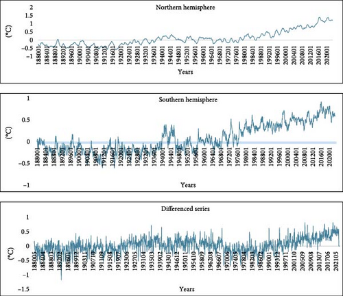
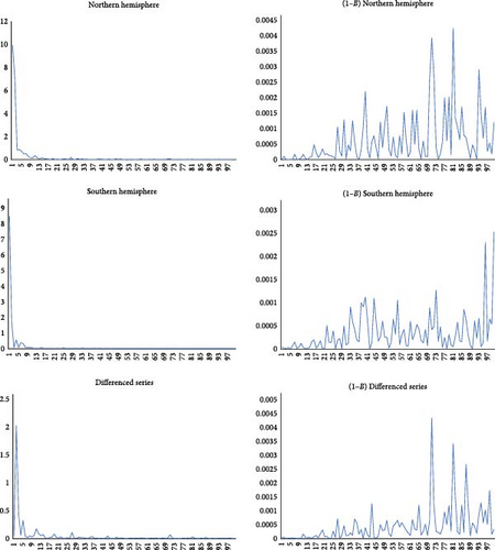
Figure 2 displays the first 100 values in the periodograms of the series. On the left are the periodograms of the three series, while those on the right correspond to the periodograms of the first differenced data. The plots on the left show a large value around the smallest (zero) frequency, which may be an indication of the need for initial differentiation. However, on the right, corresponding to the periodograms of the first differenced data, we observe values close to zero at that frequency, which may suggest that the series are now over-differenced., i.e., with no need of first differentiation. This is precisely the argument used by Granger [42] and this paper to justify the methodology employed based on fractional integration.

4. Empirical Results

We first estimate d for three potential set-ups depending on the specification of the constant and time trend in Equation (7). We first compute the values of d under the a priori assumption that α = β = 0; That is, we do not include deterministic terms in the model and y_t = x_t in the first equality in Equation (7); we then estimate d with only β = 0, so the model contains an intercept; finally, with α and β freely estimated from the data along with d, we select the correct specification across these models by the significance of the estimated coefficients using their corresponding t-values. Thus, if both coefficients are statistically significant, we choose the model with a constant and a linear time trend. However, if β is insignificant, we choose the model only with an intercept. Note here that the two first equalities in Equation (2) are jointly executed, and thus, plugging the polynomial (1–B)^d in the first of them, the errors become I (0) or short memory by assumptions, justifying the use of t-values in the regression model.

Table 1 shows the coefficients in the selected specification for each series. We see that the estimates of d differ from one series to another. Thus, for northern hemisphere temperatures, the value of d is 0.46, while for the southern hemisphere, it is much higher, 0.79, implying a much higher degree of persistence in the southern temperatures. Considering the difference between the two series, d is estimated as 0.38. The confidence intervals also indicate that while stationarity holds for the northern series and the difference between the two series, southern hemisphere temperatures are clearly non-stationary, with an order of integration much higher than 0.50. By contrast, we also see that the time trend coefficient is significantly positive for northern temperatures, statistically insignificant for southern temperatures, and positive (though with a smaller magnitude than for northern temperatures) in terms of differences. The seasonal AR coefficient is almost insignificant in the three series examined.

Table 1. Estimated coefficients in Equation (1) with data ending in December 2021.

Series	d (95% band)	Intercept (t-value)	Time trend (t-value)	Seas.
Northern hemisphere	0.46 (0.43, 0.50)	−0.32476 (−3.82)	0.00069 (6.53)	0.051
Southern hemisphere	0.79 (0.75, 0.83)	—	—	−0.037
Differences	0.38 (0.34, 0.42)	−0.15995 (−2.49)	0.00024 (3.57)	0.055

The values in parenthesis in column 2 are the 95% confidence bands of the estimates of d. Columns 3 and 4 contain the t-values of the corresponding estimates. — Means lack of significance.

Given the lack of significance in the seasonal AR coefficient, we remove this component and permit some type of weak autocorrelation for the error term. In particular, we remove the last equality in Equation (2) and assume that u_t in Equation (2) follows the approach of Bloomfield [59]. This is a non-parametric manner of assuming autocorrelation in the error term, in the sense there is no specific functional form for u_t, but is simply described by its spectral density function as follows:

(8)

and whose logged form approximates the log-spectrum of AutoRegressive (AR) structures (see Gil-Alana [60] for its application in the context of fractional integration).

Table 2 shows the results with Bloomfield’s [59]-type disturbances. The estimates for d are now slightly smaller than in the previous case, although the same conclusions hold regarding the stationarity and differences of northern hemisphere temperatures and the non-stationarity of southern temperatures. The estimates of the slope coefficients, all significant, are 0.00067 for northern, 0.00038 for southern temperatures, and 0.00024 for the difference between the two series.

Table 2. Estimated coefficients in Equation (1) with data ending in December 2021 and Bloomfield disturbances.

Series	d (95% band)	Intercept (t-value)	Time trend (t-value)
Northern hemisphere	0.49 (0.45, 0.54)	−0.30130 (−3.19)	0.00067 (5.42)
Southern hemisphere	0.70 (0.63, 0.79)	−0.01716 (−2.29)	0.00038 (1.94)
Differences	0.36 (0.32, 0.41)	−0.15897 (−2.69)	0.00024 (3.92)

In the final section, we extend the sample to incorporate the observations for the first 10 months of 2022. The results (Table 3) show very similar results to those in Table 2, with the same values for degrees of persistence and a slight increase in the slope of the time trend in the case of northern hemisphere temperatures and for the difference between the two hemispheres.

Table 3. Estimated coefficients in Equation (1) with data ending in October 2022 and Bloomfield disturbances.

Series	d (95% band)	Intercept (t-value)	Time trend (t-value)
Northern hemisphere	0.49 (0.45, 0.54)	−0.30257 (−3.21)	0.00068 (5.51)
Southern hemisphere	0.70 (0.63, 0.78)	−0.01711 (−2.29)	0.00038 (1.94)
Differences	0.36 (0.32, 0.41)	−0.16133 (−2.74)	0.00025 (4.07)

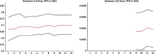
Finally, we analyse if both the degree of persistence and the time trend coefficient have changed across the sample period. For this purpose, we re-estimate the model first with data ending at 1969m12 and then adding successive 60 observations (i.e., 5 complete years) for each subsample until the end of the sample. Results for the northern and southern temperatures, and the differences between them, are shown in Figures 3, 4, and 5, respectively. The left plots display the estimates of d (and their 95% confidence intervals), while the right plots represent the β-coefficient. The lack of values in some cases in these plots refers to statistical insignificance.

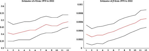
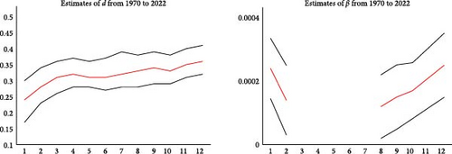
Starting with northern temperatures and focussing on d, we see a slight increase in the value of d as we increase the sample size; thus, the series seems to become more persistent over time. The same is the case in the time trend, showing a continuous increase since 1975.

For southern temperature data (Figure 4), the estimate of d has remained relatively stable over time, with an estimated d value of ~0.67, thus displaying a non-stationary pattern. The time trend coefficient is found to be statistically insignificant across most of the subsamples and only becomes significant with data ending at 2010 onwards.

Finally, for the differenced data (Figure 5), we first observe an increase in the value of the differencing parameter, moving from 0.24 (with data ending at 1969m12) to 0.36 (with data ending at 2022m10). Here, the time trend coefficient is also significant for cases with the shortest and longest subsamples.

5. Discussion

The results reported in the above section indicate substantial differences between the two hemisphere datasets. Lower degrees of persistence and more accentuated trends are observed in the northern hemisphere, where a slight increase in d is observed as we increase the sample size; that is, the series becomes more persistent over time, with the time trend coefficient being significantly positive and showing a continuous increase since 1975 in line with Shi et al. [61], which analyses temperatures in the northern hemisphere over the last 2000 years and Schlosser et al. [62], which reconstructs northern hemisphere annual temperatures since 1671 showing trends and persistence patterns. For the southern hemisphere, the estimate of d has remained relatively stable over time, showing a non-stationary pattern (values significantly above 0.5), with the time trend coefficient being statistically insignificant in most cases (it only becomes significant from 2010 onwards). By contrast, for the differenced series, we observe some evidence of stationary long memory, with an order of integration of ~0.36 and a significant positive time trend, although with a more moderate slope than in northern temperatures. Though not reported, almost identical results were obtained when using other parametric [51] or even semiparametric [63] methods when estimating the differencing parameter d, obtaining evidence of values in the interval (0, 1). These results contradict partially those papers that argue in favour of the presence of unit roots in temperature data (e.g., [24, 25]); however, it makes sense if we take into account that unit root procedure, in general, how very low power if the data are in fact fractionally integrated (see, e.g., [64, 65, 66]).

Our results suggest that, given the heterogeneity in terms of trend and persistence patterns in the temperature anomalies of both hemispheres, the policies adopted by governments to mitigate climate change should be oriented towards identifying the causes of the differences observed in the anomaly series such as the distribution of continental and oceanic masses [67], ocean currents and their influence on heat distribution [68], cyclonic activity [69], or topographic differences between hemispheres [70] and thus enable from precise and effective climate action. For example, in the event of an exogenous shock affecting temperatures, the recovery will be faster in the northern hemisphere than in the southern one, requiring stronger policy actions in the southern hemisphere to recover the original trends.

The persistence in temperature changes suggests that the northern hemisphere has a greater sensitivity to climate forcing factors, both natural and anthropogenic, which can have significant regional impacts affecting weather patterns (heat waves, cyclones, droughts) with consequences for agriculture, infrastructure, ecosystems, among others. Therefore, climate modelling must take into account the analysis of persistence so that future projections and environmental policies can be better geared to the fight against climate change. On the other hand, the differences between persistence and temperature trends in the hemispheres highlight the uneven climate change, which has implications for global climate policies.

6. Conclusions

In this paper, we have analysed northern and southern hemisphere temperature anomalies along with the difference between them in the series corresponding to the time period 1880m1 to 2022m10 using long memory processes and, in particular, a fractionally integrated modelling approach. Using this framework, we can determine the degree of persistence of the data and examine the existence of time trends from a more general and flexible view than with classical methods based on ARMA (for stationary) and ARIMA (for non-stationary) processes.

The results show substantial differences between the northern and southern hemisphere temperature data, observing lower degrees of persistence and higher time trends in the northern case. Thus, a question that emerges from these results is to understand the underlying drivers of this difference between the degrees of persistence in the two hemispheres. In this context, a fine-scale analysis can be conducted to offer valuable insights into localised climate dynamics. Future research should also incorporate potential non-linearities and structural breaks in the data. These two issues are closely related to the long memory property observed in the data ([71, 72, 73, 74], etc.), and failing to take them into account may affect the estimates of the time trends in the data.

Disclosure

A preprint of this manuscript has previously been published in Gil-Alana and Carmona-González [75].

Conflicts of Interest

There are no conflicts of interest with the publication of the present manuscript.

Acknowledgments

Prof. Luis A. Gil-Alana gratefully acknowledges financial support from the MINEIC-AEI-FEDER ECO2017-85503-R project from “Ministerio de Economía, Industria y Competitividad” (MINEIC), “Agencia Estatal de Investigación” (AEI) Spain, and “Fondo Europeo de Desarrollo Regional” (FEDER). He also acknowledges support from an internal project of the Universidad Francisco de Vitoria.

Open Research

Data Availability

The data that support the findings of this study are available from the corresponding author upon reasonable request.

References

1 World Meteorological Organization (WMO), 2022, https://public.wmo.int/en/media/press-release/eight-warmest-years-record-witness-upsurge-climate-change-impacts.
Google Scholar
2 Weather World, High temperatures exacerbated by climate change made 2022 Northern Hemisphere droughts more likely, 2022, https://www.worldweatherattribution.org/high-temperatures-exacerbated-by-climate-change-made-2022-northern-hemisphere-droughts-more-likely/.
Google Scholar
3 Broecker W. S. and Putnam A. E., Hydrologic impacts of past shifts of Earth’s thermal equator offer insight into those to be produced by fossil fuel CO₂, Proceedings of the National Academy of Sciences of the United States of America. (2013) 110, no. 42, 16710–16715, https://doi.org/10.1073/pnas.1301855110, 2-s2.0-84885777716.
10.1073/pnas.1301855110
CAS PubMed Web of Science® Google Scholar
4 IPCC, Climate Change 2021: The Physical Science Basis. Contribution of Working Group I to the Sixth Assessment Report of the Intergovernmental Panel on Climate, 2021, Change Cambridge University Press.
Google Scholar
5 Zhu J., Xie A., Qin X., Xu B., and Wang Y., Assessment of antarctic amplification based on a reconstruction of near-surface air temperature, Atmosphere. (2023) 14, no. 2, https://doi.org/10.3390/atmos14020218, 218.
10.3390/atmos14020218
Google Scholar
6 Smith D. M., Screen J. A., Deser C., Cohen J., Fyfe J. C., García-Serrano J., Jung T., Kattsov V., Matei D., Msadek R., Peings Y., Sigmond M., Ukita J., Yoon J.-H., and Zhang X., The polar amplification model intercomparison project (PAMIP) contribution to CMIP6: investigating the causes and consequences of polar amplification, Geoscientific Model Development. (2019) 12, no. 3, 1139–1164, https://doi.org/10.5194/gmd-12-1139-2019, 2-s2.0-85063428019.
10.5194/gmd-12-1139-2019
Web of Science® Google Scholar
7 Loeb N. G., Johnson G. C., Thorsen T. J., Lyman J. M., Rose F. G., and Kato S., Satellite and ocean data reveal marked increase in earth’s heating rate, Geophysical Research Letters. (2021) 48, no. 13, https://doi.org/10.1029/2021GL093047, e2021GL093047.
10.1029/2021GL093047
Web of Science® Google Scholar
8 Shaw T. A., Miyawaki O., and Donohoe A., Stormier southern Hemisphere induced by topography and ocean circulation, Proceedings of the National Academy of Sciences. (2022) 119, no. 50, https://doi.org/10.1073/pnas.2123512119, e2123512119.
10.1073/pnas.2123512119
CAS PubMed Google Scholar
9 Kornhuber K. and Tamarin-Brodsky T., Future changes in northern hemisphere summer weather persistence linked to projected arctic warming, Geophysical Research Letters. (2021) 48, no. 4, https://doi.org/10.1029/2020GL091603, e2020GL091603.
10.1029/2020GL091603
Web of Science® Google Scholar
10 Vyushin D. I. and Kushner P. J., Power-law and long-memory characteristics of the atmospheric general circulation, Journal of Climate. (2009) 22, no. 11, 2890–2904, https://doi.org/10.1175/2008JCLI2528.1, 2-s2.0-67650564914.
10.1175/2008JCLI2528.1
Web of Science® Google Scholar
11 Rypdal M. and Rypdal K., Long-memory effects in linear rypdal, response models of earth’s temperature and implications for future global warming, Journal of Climate. (2014) 27, no. 14, 5240–5258, https://doi.org/10.1175/JCLI-D-13-00296.1, 2-s2.0-84904489103.
10.1175/JCLI-D-13-00296.1
Web of Science® Google Scholar
12 Yuan N., Fu Z., and Liu S., Long-term memory in climate variability: a new look based on fractional integral techniques, Journal of Geophysical Research Atmospheres. (2014) 118, no. 23, 12962–12969, https://doi.org/10.1002/2013JD020776, 2-s2.0-84891274131.
10.1002/2013JD020776
Google Scholar
13 Yuan N., Fu Z., and Liu S., Extracting climate memory using fractional integrated statistical model: a new perspective on climate prediction, Scientific Report. (2014) 4, https://doi.org/10.1038/srep06577, 2-s2.0-84937070063, 6577.
10.1038/srep06577
CAS PubMed Web of Science® Google Scholar
14 Yuan N., Franzke C. L. E., Xiong F., Fu Z., and Dong W., The impact of long-term memory on the climate response to greenhouse gas emissions, npj Climate and Atmospheric Science. (2022) 5, https://doi.org/10.1038/s41612-022-00298-8.
10.1038/s41612-022-00298-8
PubMed Google Scholar
15 Gil-Alana L. A., Gupta R., Sauci L., and Carmona-González N., Temperature and precipitation in the US states: long memory, persistence, and time trend, Theoretical and Applied Climatology. (2022) 150, no. 3-4, 1731–1744, https://doi.org/10.1007/s00704-022-04232-z.
10.1007/s00704-022-04232-z
PubMed Web of Science® Google Scholar
16 Bloomfield P., Trends in global temperature, Climatic Change. (1992) 21, no. 1, 1–16, https://doi.org/10.1007/BF00143250, 2-s2.0-0001895030.
10.1007/BF00143250
Google Scholar
17 Brunetti M., Maugeri M., and Nanni T., Changes in total precipitation, rainy days and extreme events in northeastern Italy, International Journal of Climatology. (2001) 21, no. 7, 861–871, https://doi.org/10.1002/joc.660, 2-s2.0-0035875473.
10.1002/joc.660
Web of Science® Google Scholar
18 Folland C. K., Boucher O., Colman A., and Parker D. E., Causes of irregularities in trends of global mean surface temperature since the late 19th century, Science Advances. (2018) 4, no. 6, https://doi.org/10.1126/sciadv.aao5297, 2-s2.0-85048287497, eaao5297.
10.1126/sciadv.aao5297
PubMed Web of Science® Google Scholar
19 Gil-Alana L. A., Maximum and minimum temperatures in the United States: time trends and persistence, Atmospheric Science Letters. (2018) 19, no. 4, https://doi.org/10.1002/asl.810, 2-s2.0-85045918665.
10.1002/asl.810
PubMed Google Scholar
20 Gil-Alana L. A. and Sauci L., US temperatures: time trends and persistence, International Journal of Climatology. (2019) 39, no. 13, 5091–5103, https://doi.org/10.1002/joc.6128, 2-s2.0-85067333594.
10.1002/joc.6128
Web of Science® Google Scholar
21 Woodward W. A. and Gray H. L., Global warming and the problem of testing for trend in time series data, Journal of Climate. (1993) 6, no. 5, 953–962, https://doi.org/10.1175/1520-0442(1993)006%3C0953:GWATPO%3E2.0.CO;2.
10.1175/1520-0442(1993)006<0953:GWATPO>2.0.CO;2
Web of Science® Google Scholar
22 Stern D. I. and Kaufmann R. K., Detecting a global warming signal in hemispheric temperature series: a structural time series analysis, Climatic Change. (2000) 47, no. 4, 411–438, https://doi.org/10.1023/A:1005672231474, 2-s2.0-0033767771.
10.1023/A:1005672231474
Web of Science® Google Scholar
23 Hamdi R., Kusaka H., Doan Q.-V., Cai P., He H., Luo G., Kuang W., Caluwaerts S., Duchêne Fçois, Van Schaeybroek B., and Termonia P., The state-of-the-art of urban climate change modeling and observations, Earth Systems and Environment. (2020) 4, no. 4, 631–646, https://doi.org/10.1007/s41748-020-00193-3.
10.1007/s41748-020-00193-3
Google Scholar
24 Cummins D. P., Stephenson D. B., and Stott P. A., Could detection and attribution of climate change trends be spurious regression?, Climate Dynamics. (2022) 59, no. 9-10, 2785–2799, https://doi.org/10.1007/s00382-022-06242-z.
10.1007/s00382-022-06242-z
PubMed Google Scholar
25 McKitrick R., Vogelsang T., and Christy J., Temperature trends, climate attribution and the nonstationarity question, Earth System Dynamics, 2023, [preprint].
Google Scholar
26 Fomby T. B. and Vogelsang T. J., The application of size-robust trend statistics to global-warming temperature series, Journal of Climate. (2002) 15, no. 1, 117–123, https://doi.org/10.1175/1520-0442(2002)015%3C0117:TAOSRT%3E2.0.CO;2.
10.1175/1520-0442(2002)015<0117:TAOSRT>2.0.CO;2
Web of Science® Google Scholar
27 Fatichi S., Barbosa S. M., Caporali E., and Silva M. E., Deterministic versus stochastic trends: detection and challenges, Journal of Geophysical Research. (2009) 114, no. D18, https://doi.org/10.1029/2009JD011960, 2-s2.0-72049125637, D18121.
10.1029/2009JD011960
Web of Science® Google Scholar
28 Weber R. O. and Talkner P., Spectra and correlations of climate data from days to decades, Journal of Geophysical Research. (2001) 106, no. D17, 20131–20144, https://doi.org/10.1029/2001JD000548, 2-s2.0-0034773050.
10.1029/2001JD000548
Web of Science® Google Scholar
29 Kantelhardt J. W., Koscielny-Bunde E., Rego H. H. A., Havlin S., and Bunde A., Detecting long-range correlations with detrended fluctuation analysis, Physica A: Statistical Mechanics and its Applications. (2001) 295, no. 3-4, 441–454, https://doi.org/10.1016/S0378-4371(01)00144-3, 2-s2.0-0035876536.
10.1016/S0378-4371(01)00144-3
Web of Science® Google Scholar
30 Yuan N., Ding M., Huang Y., Fu Z., Xoplaki E., and Luterbacher J., On the long-term climate memory in the surface air temperature records over antarctica: a nonnegligible factor for trend evaluation, Journal of Climate. (2015) 28, no. 15, 5922–5934, https://doi.org/10.1175/JCLI-D-14-00733.1, 2-s2.0-84942917272.
10.1175/JCLI-D-14-00733.1
Web of Science® Google Scholar
31 Massah M. and Kantz H., Confidence intervals for time averages in the presence of long-range correlations, a case study on Earth surface temperature anomalies, Geophysical Research Letters. (2016) 43, no. 17, 9243–9249, https://doi.org/10.1002/2016GL069555, 2-s2.0-84988980310.
10.1002/2016GL069555
Web of Science® Google Scholar
32 Bloomfield P. and Nychka D., Climate spectra and detecting climate change, Climatic Change. (1992) 21, no. 3, 275–287, https://doi.org/10.1007/BF00139727, 2-s2.0-0001450102.
10.1007/BF00139727
Web of Science® Google Scholar
33 Vogelsang T. J. and Franses P. H., Are winters getting warmer?, Environmental Modelling and Software. (2005) 20, no. 11, 1449–1455, https://doi.org/10.1016/j.envsoft.2004.09.016, 2-s2.0-16244419430.
10.1016/j.envsoft.2004.09.016
Web of Science® Google Scholar
34 Gil-Alana L. A., Statistical modeling of the temperatures in the northern hemisphere using fractional integration techniques, Journal of Climate. (2005) 18, no. 24, 5357–5369, https://doi.org/10.1175/JCLI3543.1, 2-s2.0-31544439625.
10.1175/JCLI3543.1
Web of Science® Google Scholar
35 Gil-Alana L. A., Warming break trends and fractional integration in the northern, southern, and global temperature anomaly series, Journal of Atmospheric and Oceanic Technology. (2008) 25, no. 4, 570–578, https://doi.org/10.1175/2007JTECHA1025.1, 2-s2.0-45749133085.
10.1175/2007JTECHA1025.1
Web of Science® Google Scholar
36 Hare S. R. and Mantua N. J., Empirical evidence for North Pacific regime shifts in 1977 and 1989, Progress in Oceanography. (2000) 47, no. 2–4, 103–145, https://doi.org/10.1016/S0079-6611(00)00033-1, 2-s2.0-0033744926.
10.1016/S0079-6611(00)00033-1
Web of Science® Google Scholar
37 Alley R. B., Marotzke J., Nordhaus W. D., Overpeck J. T., Peteet D. M., PielkeR. A.Jr., Pierrehumbert R. T., Rhines P. B., Stocker T. F., Talley L. D., and Wallace J. M., Abrupt climate change, Science. (2003) 299, no. 5615, 2005–2010, https://doi.org/10.1126/science.1081056, 2-s2.0-0037471002.
10.1126/science.1081056
CAS PubMed Web of Science® Google Scholar
38 Jiang L., Li N., and Zhao X., Scaling behaviors of precipitation over China, Theoretical and Applied Climatology. (2017) 128, 63–70, https://doi.org/10.1007/s00704-015-1689-2, 2-s2.0-84949950962.
10.1007/s00704-015-1689-2
Web of Science® Google Scholar
39 Chen X., Lin G., and Fu Z., Long-range correlations in daily relative humidity fluctuations: a new index to characterize the climate regions over China, Geophysical Research Letters. (2007) 34, no. 7, https://doi.org/10.1029/2006GL027755, 2-s2.0-34250728628, L07804.
10.1029/2006GL027755
Web of Science® Google Scholar
40 Caporale G. M., Gil-Alana L. A., and Carmona-González N., Particulate matter 10 (PM₁₀): persistence and trends in eight European capitals, Air Quality Atmosphere & Health. (2021) 14, no. 7, 1097–1102, https://doi.org/10.1007/s11869-021-01002-0.
10.1007/s11869-021-01002-0
CAS Google Scholar
41 Mandelbrot B. B. and Van Ness J. W., Fractional Brownian motions, fractional noises and applications, SIAM Review. (1968) 10, no. 4, 422–437, https://doi.org/10.1137/1010093.
10.1137/1010093
Web of Science® Google Scholar
42 Granger C. W. J., Long memory relationships and the aggregation of dynamic models, Journal of Econometrics. (1980) 14, no. 2, 227–238, https://doi.org/10.1016/0304-4076(80)90092-5, 2-s2.0-0018872157.
10.1016/0304-4076(80)90092-5
Web of Science® Google Scholar
43 Granger C. W. J., Some properties of time series data and their use in econometric model specification, Journal of Econometrics. (1981) 16, no. 1, 121–130, https://doi.org/10.1016/0304-4076(81)90079-8, 2-s2.0-49149136839.
10.1016/0304-4076(81)90079-8
Web of Science® Google Scholar
44 Granger C. W. J. and Joyeux R., An introduction to long-memory time series models and fractional differencing, Journal of Time Series Analysis. (1980) 1, no. 1, 15–29, https://doi.org/10.1111/j.1467-9892.1980.tb00297.x, 2-s2.0-84986792205.
10.1111/j.1467-9892.1980.tb00297.x
Google Scholar
45 Hosking J. R. M., Fractional differencing, Biometrika. (1981) 68, no. 1, 165–176, https://doi.org/10.1093/biomet/68.1.165, 2-s2.0-77956890381.
10.1093/biomet/68.1.165
Web of Science® Google Scholar
46 Hurst H. E., Long-term storage capacity of reservoirs, Transactions of the American Society of Civil Engineers. (1951) 116, no. 1, 770–799, https://doi.org/10.1061/TACEAT.0006518.
10.1061/TACEAT.0006518
Web of Science® Google Scholar
47 Lo A. W., Long-term memory in stock market prices, Econometrica. (1991) 59, no. 5, 1279–1313, https://doi.org/10.2307/2938368.
10.2307/2938368
Web of Science® Google Scholar
48 Geweke J. and Porter-Hudak S., The estimation and application of long memory time series models, Journal of Time Series Analysis. (1983) 4, no. 4, 221–238, https://doi.org/10.1111/j.1467-9892.1983.tb00371.x, 2-s2.0-84986759400.
10.1111/j.1467-9892.1983.tb00371.x
Google Scholar
49 Robinson P. M., Log periodogram regression of time series with long range dependence, The Annals of Statistics. (1995) 23, no. 3, 1048–1072, https://doi.org/10.1214/aos/1176324636.
10.1214/aos/1176324636
Web of Science® Google Scholar
50 Kim C. S. and Phillips P. C. B., Log periodogram regression: the nonstationary case (October 2006). Cowles foundation discussion paper no. 1587, 2006, Available at SSRN: https://ssrn.com/abstract=937915.
Google Scholar
51 Sowell F., Maximum likelihood estimation of stationary univariate fractionally integrated time series models, Journal of Econometrics. (1992) 53, no. 1–3, 165–188, https://doi.org/10.1016/0304-4076(92)90084-5, 2-s2.0-44049114907.
10.1016/0304-4076(92)90084-5
Web of Science® Google Scholar
52 Robinson P. M., Efficient tests of nonstationary hypotheses, Journal of the American Statistical Association. (1994) 89, no. 428, 1420–1437, https://doi.org/10.1080/01621459.1994.10476881, 2-s2.0-84923145850.
10.1080/01621459.1994.10476881
Web of Science® Google Scholar
53 Gil-Alaña L. A. and Robinson P. M., Testing of unit root and other nonstationary hypotheses in macroeconomic time series, Journal of Econometrics. (1997) 80, no. 2, 241–268, https://doi.org/10.1016/S0304-4076(97)00038-9, 2-s2.0-30244432554.
10.1016/S0304-4076(97)00038-9
Web of Science® Google Scholar
54 Gil-Alana L., Estimation of the degree of dependence in the temperatures in the northern hemisphere using semi-parametric techniques, Journal of Applied Statistics. (2003) 30, no. 9, 1021–1031, https://doi.org/10.1080/0266476032000076146, 2-s2.0-0142244675.
10.1080/0266476032000076146
Web of Science® Google Scholar
55 Toggweiler J. R. and Lea D. W., Temperature diffeences between the hemispheres and ice age climate variability, Paleoceanography and Paleoclimatology. (2010) 25, no. 2, https://doi.org/10.1029/2009PA001758, 2-s2.0-77952660600, PA2212.
10.1029/2009PA001758
Web of Science® Google Scholar
56 Feulner G., Rahmstorf S., Levermann A., and Volkwardt S., Why is the northern hemisphere warmer than the southern hemisphere, discussion paper, 2013, https://www.researchgate.net/publication/258778329.
Google Scholar
57 Yasmeen F., Measuring global warming: global and hemisphere mean temperature anomalies predictions using sliced functional time series (SFTS) model, Open Journal of Applied Sciences. (2019) 9, no. 5, 316–334, https://doi.org/10.4236/ojapps.2019.95026.
10.4236/ojapps.2019.95026
Google Scholar
58 Miller R. L., Lackmann G. M., and Robinson W. A., A new variable-threshold persistent anomaly index: northern hemisphere anomalies in the ERA-interim reanalysis, Monthly Weather Review. (2020) 148, no. 1, 43–62, https://doi.org/10.1175/MWR-D-19-0144.1.
10.1175/MWR-D-19-0144.1
Web of Science® Google Scholar
59 Bloomfield P., An exponential model in the spectrum of a scalar time series, Biometrika. (1973) 60, no. 2, 217–226, https://doi.org/10.1093/biomet/60.2.217, 2-s2.0-0015894045.
10.1093/biomet/60.2.217
Web of Science® Google Scholar
60 Gil-Alana L. A., Fractional integration with Bloomfield exponential spectral disturbances. A Monte Carlo experiment and an application, Brazilian Journal of Probability and Statistics. (2008) 22, no. 1, 69–83.
Google Scholar
61 Shi F., Ting M., and Guo Z., Quantitative attribution of northern hemisphere temperatures over the past 2000 years, Frontiers of Earth Science. (2023) 17, no. 2, 632–641, https://doi.org/10.1007/s11707-023-1086-6.
10.1007/s11707-023-1086-6
Google Scholar
62 Schlosser A., Sokolov A., Strzepek K., Thomas T., Gao X., and Arndt C., The changing nature of hydroclimatic risks across South Africa, Climatic Change. (2021) 168, no. 3-4, https://doi.org/10.1007/s10584-021-03235-5, 28.
10.1007/s10584-021-03235-5
Google Scholar
63 Shimotsu K. and Phillips P. C. B., Exact local Whittle estimation of fractional integration, The Annals of Statistics. (2005) 33, no. 4, 1890–1933, https://doi.org/10.1214/009053605000000309, 2-s2.0-26444501037.
10.1214/009053605000000309
Web of Science® Google Scholar
64 Diebold F. X. and Rudebusch G. D., On the power of Dickey-Fuller test against fractional alternatives, Economics Letters. (1991) 35, 155–160, https://doi.org/10.1016/0165-1765(91)90163-F, 2-s2.0-0000289304.
10.1016/0165-1765(91)90163-F
Web of Science® Google Scholar
65 Hasslers U. and Wolters J., On the power of unit root tests against fractional alternatives, Economics Letters. (1994) 45, no. 1, 1–5, https://doi.org/10.1016/0165-1765(94)90049-3, 2-s2.0-21344476815.
10.1016/0165-1765(94)90049-3
Web of Science® Google Scholar
66 Lee D. and Schmidt P., On the power of the KPSS test of stationarity against fractionally-integrated alternatives, Journal of Econometrics. (1996) 73, no. 1, 285–302, https://doi.org/10.1016/0304-4076(95)01741-0, 2-s2.0-0000495205.
10.1016/0304-4076(95)01741-0
Web of Science® Google Scholar
67 Trenberth K. E. and Caron J. M., Estimates of meridional atmosphere and ocean heat transports, Journal of Climate. (2001) 14, no. 16, 3433–3443, https://doi.org/10.1175/1520-0442(2001)014%3C3433:EOMAAO%3E2.0.CO;2.
10.1175/1520-0442(2001)014<3433:EOMAAO>2.0.CO;2
Web of Science® Google Scholar
68 Marshall J. and Speer K., Closure of the meridional overturning circulation through Southern Ocean upwelling, Nature Geoscience. (2012) 5, no. 3, 171–180, https://doi.org/10.1038/ngeo1391, 2-s2.0-84857867380.
10.1038/ngeo1391
CAS PubMed Web of Science® Google Scholar
69 Priestley M. D. K. and Catto J. L., Future changes in the extratropical storm tracks and cyclone intensity, wind speed, and structure, Weather and Climate Dynamics. (2022) 3, no. 1, 337–360, https://doi.org/10.5194/wcd-3-337-2022.
10.5194/wcd-3-337-2022
Google Scholar
70 You Q., Cai Z., Pepin N., Chen D., Ahrens B., Jiang Z., Wu F., and Kang S., et al.Warming amplification over the Arctic Pole and Third Pole: trends, mechanisms and consequences, Earth-Science Reviews. (2021) 17, https://doi.org/10.1016/j.earscirev.2021.103625, 103625.
10.1016/j.earscirev.2021.103625
Google Scholar
71 Deo R., Hsieh M., Hurvich C. M., and Soulier P., P. Bertail, P. Soulier, and P. Doukhan, Long memory in nonlinear processes, Dependence in Probability and Statistics. Lecture Notes in Statistics, 2006, 187, Springer, New York, https://doi.org/10.1007/0-387-36062-X_10.
10.1007/0-387-36062-X_10
Google Scholar
72 Diebold F. X. and Inoue A., Long memory and regime switching, Journal of Econometrics. (2001) 105, no. 1, 131–159, https://doi.org/10.1016/S0304-4076(01)00073-2, 2-s2.0-0001418135.
10.1016/S0304-4076(01)00073-2
Web of Science® Google Scholar
73 Granger C. W. J. and Hyung N., Occasional structural breaks and long memory with an application to the S&P 500 absolute stock returns, Journal of Empirical Finance. (2004) 11, no. 3, 399–421, https://doi.org/10.1016/j.jempfin.2003.03.001, 2-s2.0-1942444547.
10.1016/j.jempfin.2003.03.001
Google Scholar
74 Chatzikonstanti V. and Venetis I. A., Long memory in log-range series: do structural breaks matter?, Journal of Empirical Finance. (2015) 33, 104–113, https://doi.org/10.1016/j.jempfin.2015.06.003, 2-s2.0-84939473579.
10.1016/j.jempfin.2015.06.003
Google Scholar
75 Gil-Alana L. A. and Carmona-González N., Temperature anomalies in the northern and southern hemispheres. Evidence of persistence and trends, Research Square. (2023) https://doi.org/10.21203/rs.3.rs-3256176/v1.
10.21203/rs.3.rs-3256176/v1
Google Scholar

All articles

Temperature Anomalies in the Northern and Southern Hemispheres: Evidence of Persistence and Trends

Abstract

1. Introduction

2. A Review of the Literature

3. Materials and Methods

3.1. Data

4. Empirical Results

5. Discussion

6. Conclusions

Disclosure

Conflicts of Interest

Acknowledgments

Open Research

Data Availability

References

Figures

References

Information

About Wiley Online Library

Help & Support

Opportunities

Connect with Wiley

Temperature Anomalies in the Northern and Southern Hemispheres: Evidence of Persistence and Trends

Abstract

1. Introduction

2. A Review of the Literature

3. Materials and Methods

3.1. Data

4. Empirical Results

5. Discussion

6. Conclusions

Disclosure

Conflicts of Interest

Acknowledgments

Open Research

Data Availability

References

Figures

References

Related

Information